Human Capital Development Before Age Five

NBER WORKING PAPER SERIES

HUMAN CAPITAL DEVELOPMENT BEFORE AGE FIVE Douglas Almond

Janet Currie Working Paper 15827

http://www.nber.org/papers/w15827

NATIONAL BUREAU OF ECONOMIC RESEARCH 1050 Massachusetts Avenue

Cambridge, MA 02138 March 2010

We thank Maya Rossin and David Munroe for excellent research assistance, participants in the Berkeley Handbook of Labor Economics Conference in November 2009 for helpful comments, and Christine Pal and Hongyan Zhao for proofreading the equations. The views expressed herein are those of the authors and do not necessarily reflect the views of the National Bureau of Economic Research. NBER working papers are circulated for discussion and comment purposes. They have not been peer-reviewed or been subject to the review by the NBER Board of Directors that accompanies official NBER publications.

© 2010 by Douglas Almond and Janet Currie. All rights reserved. Short sections of text, not to exceed two paragraphs, may be quoted without explicit permission provided that full credit, including © notice, is given to the source.

Human Capital Development Before Age Five Douglas Almond and Janet Currie

NBER Working Paper No. 15827 March 2010, Revised January 2011 JEL No. I12,I21,J13,J24,Q53

ABSTRACT

This chapter seeks to set out what Economists have learned about the effects of early childhood influences on later life outcomes, and about ameliorating the effects of negative influences. We begin with a brief overview of the theory which illustrates that evidence of a causal relationship between a shock in early childhood and a future outcome says little about whether the relationship in question biological or immutable. We then survey recent work which shows that events before five years old can have large long term impacts on adult outcomes. Child and family characteristics measured at school entry do as much to explain future outcomes as factors that labor economists have more traditionally focused on, such as years of education. Yet while children can be permanently damaged at this age, an important message is that the damage can often be remediated. We provide a brief overview of evidence regarding the effectiveness of different types of policies to provide remediation. We conclude with a list of some of (the many) outstanding questions for future research.

Douglas Almond

Department of Economics Columbia University

International Affairs Building, MC 3308 420 West 118th Street

New York, NY 10027 and NBER

[email protected] Janet Currie

International Affairs Building Department of Economics

Columbia University - Mail code 3308 420 W 118th Street

New York, NY 10027 and NBER

1

Introduction

The last decade has seen a blossoming of research on the long term effects of early childhood conditions across a range of disciplines. In economics, the focus is on how hu-man capital accumulation responds to the early childhood environment. In 2000, there were no articles on this topic in the Journal of Political Economy, Quarterly Journal of Economics,orthe American Economic Review (excluding the Papers and Proceedings), but there have been five or six per year in these journals since 2005. This work has been spurred by a growing realization that early life conditions can have persistent and profound impacts on later life. Table 1 summarizes several longitudinal studies which suggest that characteristics that are measured as of age 7 can explain a great deal of the variation in educational attainment, earnings as of the early 30s, and the probability of employment. For example, McLeod and Kaiser [2004] use data from the National Longi-tudinal Surveys and find that children’s test scores and background variables measured as of ages 6 to 8 predict about 12% of the variation in the probability of high school completion and about 11% of the variation in the probability of college completion. Currie and Thomas [1999a] use data from the 1958 British Birth Cohort study and find that 4 to 5% of the variation in employment at age 33 can be predicted, and as much as 20% of the variation in wages. Cunha and Heckman [2008] and Cunha, Heckman, and Schennach [forthcoming] estimate structural models in which initial endowments and investments feed through to later outcomes; they arrive at estimates that are of a similar order of magnitude for education and wages. To put these results in context, labor economists generally feel that they are doing well if they can explain 30% of the variation in wages in a human capital earnings function.

This chapter seeks to set out what economists have learned about the importance of early childhood influences on later life outcomes, and about ameliorating the effects of negative influences. We begin with a brief overview of the theory which illustrates that evidence of a causal relationship between a shock in early childhood and a future outcome says little about whether the relationship in question biological or immutable. Parental and social responses are likely to be extremely important in either magnifying or mitigating the effects of a shock. Given that this is the case, it can sometimes be difficult to interpret the wealth of empirical evidence that is accumulating in terms of an underlying structural framework.

The theoretical framework is laid out in Section 3 and followed by a brief discussion of methods in Section 4. We do not attempt to cover issues such as identification and instrumental variables methods which are covered in some depth elsewhere (cf Angrist and Pischke [2009]). Instead, we focus on several issues that come up frequently in the

early influences literature, including estimation using small samples and the potentially high return to better data.

The fifth section of the paper discusses the evidence for long term effects of early life influences in greater detail, while the sixth focuses on the evidence regarding reme-diation programs. The discussion of early life influences is divided into two sections corresponding toin utero influences and after birth influences. The discussion of reme-diation programs starts from the most general sort of program, income transfers, and goes on to discuss interventions that are increasingly targeted at specific domains. In surveying the evidence we have attempted to focus on recent papers, and especially those that propose a plausible strategy for identifying causal effects. We have focused on papers that emphasize early childhood, but in instances in which only evidence re-garding effects on older children is available, we have sometimes strayed from this rule. A summary of most of the papers discussed in these sections is presented in Tables 4 through 13. A list of acronyms used in the tables appears in Appendix A. We conclude with a summary and a discussion of outstanding questions for future research in Section 7.

2

Conceptual Framework

Grossman [1972] models health as a stock variable that varies over time in response to investments and depreciation. Because some positive portion of the previous period’s health stock vanishes in each period (e.g., age in years), the effect of the health stock and health investments further removed in time from the current period tends to fade out. As individuals age, the early childhood health stock and the prior health investments that it embodies become progressively less important.

In contrast, the “early influences” literature asks whether health and investments in early childhood have sustained effects on adult outcomes. The magnitude of these effects may persist or even increase as individuals age because childhood development occurs in distinct stages that are more or less influential of adult outcomes.

Defining h as health or human capital at the completion of childhood, we can retain the linearity of h in investments and the prior health stock as in Grossman [1972], but leave open whether there is indeed “fade out” (i.e. depreciation). For simplicity, we will consider a simple two-period childhood.1 _{We can consider production of h:}

h=A[γI1+ (1−γ)I2], (1)

where:

(

I1 ∼= investments during childhood through age 5 I2 ∼= investments during childhood after age 5.

For a given level of total investments I1 +I2, the allocation of investments between period 1 and 2 will also affect h for γ 6=.5. If γ > .5, then health at the end of period 1 is more important to h than investments in the second period, and if γA >1, h may respond more than one-for-one with I1. Thus, (1) admits the possibility that certain childhood periods may exert a disproportionate effect on adult outcomes that does not necessarily decline monotonically with age. This functional form says more than “early life” matters; it suggests that early-childhood events may be more influential than later childhood events.

2.1

Complementarity

The assumption that inputs at different stages of childhood have linear effects is common in economics. While it opens the door to “early origins”, perfect substitutability between first and second period investments in (1) is a strong assumption. The absence of complementarity implies that all investments should be concentrated in one period (up to a discount factor) and no investments should be made during the low-return period. In addition, with basic preference assumptions, perfect substitutability “hard-wires” the optimal investment response to early-life shocks to be compensatory, as seen in Section 2.3.

As suggested by Heckman [2007], a more flexible “developmental” technology is the constant elasticity of substitution (CES) function:

h =A h

γI₁φ+ (1−γ)I₂φ i1/φ

, (2)

For a given total investment level I1 +I2, how the allocation between period 1 and 2 will also affect h depends on the elasticity of substitution,1/(1− φ),and the share parameter,γ. For φ = 1 (perfect substitutability of investments), (2) reduces to (1).

Heckman [2007] highlights two features of “capacity formation” beyond those cap-tured in (2). First, there may be “dynamic complementarities” which imply that in-vestments in period t are more productive when there is a high level of capability in period t−1. For example, if the factor productivity term A in (2) were an increasing function of h0, the health endowment immediately prior to period 1, this would raise the return to investments during childhood. Second, there may be “self-productivity” which implies that higher levels of capacity in one period create higher levels of capacity

in future periods. This feature is especially noteworthy when h is multidimensional, as it would imply that “cross-effects” are positive, e.g. health in period 1 leads to higher cognitive ability in period 2. “Self-productivity” is more trivial in the unidimensional case like Grossman [1972] – even though the effect of earlier health stocks tends to fade out as the time passes, there is still memory as long as depreciation in each period is less than total (i.e., when δ <1 in Zweifel, Breyer, and Kifmann [2009]).

Here, we will use the basic framework in (2) to consider the effect of exogenous shocks µ_g to health investments that occur during the first childhood period.2 We begin with the simplest case, where investments do not respond toµ_g (and denote these investments

¯

I1 and ¯I2). Net investments in the first period are: ¯

I1+µ_g.

We assume that µ_g is independent of ¯I1. While µg can be positive or negative, we

assume ¯I1 +µg > 0. We will then relax the assumption of fixed investments, and

consider endogenous responses to investments in the second period, i.e. δI₂∗/δµ_g, and how this investment response may mediate the observed effect on h.

2.2

Fixed Investments

Conceptually, we can trace out the effect of µ_g while holding other inputs fixed, i.e., we assume no investment response to this shock in either period. Albeit implicitly, most biomedical and epidemiological studies in the “early origins” literature aim to inform us about thisceteris paribus, “biological” relationship.

In this two-period CES production function adopted from Heckman [2007], the im-pact of an early-life shock on adult outcomes is:

δh δµ_g =γA h γ( ¯I1+µg) φ_{+ (1−γ) ¯I}φ 2 i(1−φ)/φ ( ¯I1+µg) φ−1_{. (3)} The simplest production technology is the perfect substitutability case where φ= 1. In this case:

δh

δµ_g =γA.

Damage to adult human capital is proportional to the share parameter on period 1 investments, and is unrelated to the investment level ¯I1.

2_{We include the subscript here because environmental influences at some aggregated geographic level}

For less than perfect substitutability between periods, there is diminishing marginal productivity of the investment inputs. Thus, shocks experienced at different baseline investment levels have heterogenous effects on h. Other things equal, those with higher baseline levels of investment will experience more muted effects in h than those where baseline investment is low. A recurring empirical finding is that long-term damage due to shocks is more likely among poorer families [Currie and Hyson, 1999]. This is in part due to the fact that children in poorer families are subject to more or larger early-life shocks [Case, Lubotsky, and Paxson, 2002, Currie and Stabile, 2003]. However, it is also possible that the same shock will have a greater impact among children in poorer families if these children have lower periodtinvestment levels to begin with. This occurs because they are on a steeper portion of the production function. Ceteris paribus, this would tend to accentuate the effect of an equivalent-sized µ_g shock on h among poor families.3,4

2.2.1 Remediation

Is it possible to alter “bad” early trajectories? In other words, what is the effect of a shock µ0_g >0 experienced during the second period on h? Remediation is of interest to the extent that (3) is substantially less than zero. However, large damage to h from µ_g per se says little about the potential effectiveness of remediation in the second period as both initial damage and remediation are distinct functions of the three parameters A, γ, and φ.

The effectiveness of remediation relative to initial damage is:

δh/δµ0_g δh/δµ_g = 1−γ γ ¯ I1+µ_g ¯ I2+µ 0 g !1−φ . (4)

Thus, for ¯I1 >I¯2 and a given value of γ, a unit of remediation will be more effective at low elasticities of substitution – the lack of ¯I2 was the more critical shortfall prior to the shock. If ¯I1 < I¯2 high elastiticites of substitution increase the effectiveness of remediation – adding to the existing abundance of ¯I2 remains effective.

Fortunately, it is not necessary to observe investments and estimate all three pa-rameters in order to assess the scope for remediation. In some cases, we merely need

3_{i.e. δ}2_h/δµ

gδI1 <0. On the other hand,δ2h/δµgδI2 >0 so lower period two investments would tend to reduce damage to h from µ_g. The ratio of the former effect to the latter is proportional to

γ/(1−γ) [Chiang, 1984]. Thus, damage from a period 1 shock is more likely to be concentrated among poor families when the period-1 share parameter (γ) is high.

4_{The cross-effect δ}2

h/δµ_gδI2 is similar to dynamic complementarity, but Heckman [2007] reserves this term for the cross-partial between the stock and flow, i.e. δ2h/δh0δIt for t=1,2 in the example of

to observe how a shock in the second period, µ0_g, affects h. Furthermore, this does not necessarily require a distinct shock in addition to µ_g. In an overlapping generations framework, the same shock, µ_g = µ_g0 could affect one cohort in the first childhood pe-riod (but not the second) and an older cohort in the second pepe-riod (but not the first). For a small, “double-barrelled” shock, we would have a reduced form estimates of both the damage in (3) and the potential to alter trajectories in (4).5 _{For example, in} addi-tion to observing how income during the prenatal period affects newborn health [Kehrer and Wolin, 1979], we might also be able to see how parental income affects the health of pre-school age children to gain a sense of what opportunities there are to remediate negative income shocks experienced during pregnancy.

2.3

Responsive Investments

Most analyses of “early origins” focus on estimating the reduced form effect, δh/δµ_g. Whether this empirical relationship represents a purely biological effect or also includes the effect of responsive investments is an open question. In general, to the extent that “early origins” are important, so too will any response of childhood investments to µ_g. For expositional purposes, we will consider µ_g <0 and responses that either magnify or attenuate initial damage.

Unless the investment response is costless, damage estimates which monetizeδh/δµ_g alone will tend to understate total damage. In the extreme, investment responses could fully offset the effect of early-life shocks on h but this would not mean that such shocks were costless [Deschnes and Greenstone, 2007]. More generally, the damage from early-life shocks will be understated if we focus only on long-term effects and there are com-pensatory investments (i.e. investments that are negatively correlated with the early-life shock (δI₂∗/δµ_g <0)). The cost of investments which help remediate damage should be included. But even when the response is reinforcing (δI₂∗/δµ_g >0), total costs can still be understated by focussing on the reduced form damage to h alone (see below).

To consider correlated investment responses more formally, we assume parents ob-serve µ_g at the end of the first period. The direction of the investment response – whether reinforcing or compensatory – will be shaped by how substitutable period 2 investments are for those in period 1. If substitutability is high, the optimal response will tend to be compensatory, and thereby help offset damage to h.

A compensatory response is readily seen in the case of perfect substitutability. Cunha and Heckman [2007] observed that economic models commonly assume that production

at different stages of childhood are perfect substitutes. When φ= 1, (2) reduces to:

h=Aγ(I1+µg) + (1−γ)I2

. (5)

This linear production technology is akin to that used in a previousHandbook chapter on intergenerational mobility [Solon, 1999], which likewise considered parental invest-ments in children’s human capital. Further, Solon [1999] assumed parent’s utility trades off own consumption against the child’s human capital:

Up =U(C, h), (6)

where pdenotes parents and C their consumption. The budget constraint is:

Yp =C+I1+I2/(1 +r). (7)

With standard preferences, changes to h through µ_g will “unbalance” the marginal utilities in h versus C.6 _{If µ}

g is negative, the marginal utility of h becomes too high

relative to that in consumption. The technology in (5) permits parents to convert some consumption into h at a constant rate. This will cause I₂∗ to increase, which attenuates the effect of the µ_g damage. This attenuation comes at the cost of reduced parental utility. Similarly, if µ_g is positive parents will “spend the bounty” (at least in part), reduce I₂∗ and increase consumption. Again, this will temper effects on h, leading to an understatement of biological effects in analyses that ignore investments (or parental utility). In either case, perfect substitutability hard-wires the response to be compensatory.

The polar opposite technology is perfect complementarity between childhood stages, i.e., a Leontieff production function. Here, a compensatory strategy would be completely ineffective in mitigating changes toh. Ashis determined by the minimum of period 1 and period 2 investments, optimal period 2 investments should reinforceµ_g. Ifµ_g is negative, parents would seek to reduceI2and consume more. Despite higher consumption, parents’ utility is reduced on net due to the shock (or this bundle of lower hand higher C would have been selected absentµ_g). Again, the full-cost of a negativeµ_g shock is understated when parental utility is ignored.

The crossover between reinforcing and compensating responses of I₂∗ will occur at an intermediate parameter value of substitutability. (The fixed investments case of Section 2.2 can be seen to reflect an optimized response at this point of balance between 6_{Obviously, the marginal utilities themselves will not be the same but equal subject to discount} factor, preference parameters, and prices ofC versusI which have been ignored.

reinforcing and compensating responses). The value of φ at this point of balance will depend on the functional form of parental preferences in (6), as shown for CES utility in Appendix B.

To take a familiar example, assume a Cobb-Douglas utility function of the form:

Up = (1−α)logC+αlogh. (8)

If the production technology is also Cobb-Douglas (φ = 0), then no change to I₂∗ is warranted. If instead substitution between period 1 and period 2 is relatively easy (φ > 0), compensating for the shock is optimal. If substitution is relatively difficult (φ <0), then parents should “go with the flow” and reinforce. For this reason, whether conventional reduced form analyses under or over-state “biological” effects (effects with I2 held fixed) depends on how easy it is to substitute the timing of investments across childhood. If the elasticity of substitution across periods is low, then it may be optimal for parents to reinforce the effect of a shock.

Tension between preferences and the production technology may also be relevant for within-family investment decisions. For example, Behrman, Pollak, and Taubman [1982] considered parental preferences that parameterize varying degrees of “inequality aversion” among (multiple) children. Depending on the strength of parents’ inequality aversion relative to the production technology (as reflected by φ), parents may rein-force or compensate exogenous within-family differences in early-life health and human capital. If substitutability between periods of childhood is sufficiently difficult (low φ), reinforcement of sibling differences will be optimal. This reinforcement may be optimal even when the parents place a higher weight in their utility function on the accumulation of human capital by the less able sibling (see Appendix C). Thus, empirical evidence that some parents reinforce early-life shocks could reveal less about “human nature” than it would reveal about the developmental nature of the childhood production technology.

3

Methods

As discussed above, we confine our discussion to methodological issues that seem par-ticularly germane to the early influences literature. One of these is the question of when sibling fixed effects (or maternal fixed effects) estimation is appropriate. Fixed effects can be a powerful way to eliminate confounding from shared family background characteristics, even when these are not fully observed. This approach is particularly effective when the direction of unobserved sibling-specific confounders can be signed.

For example, Currie and Thomas [1995] find that in the cross-section, children who were in Head Start do worse than children who were not. However, compared to their own siblings, Head Start children do better. Since there is little evidence that Head Start children are “favored” by parents or otherwise (on the contrary, in families where one child attends and the other does not, children who attended were more likely to have spent their preschool years in poverty), these contrasting results suggest that unob-served family characteristics are correlated both with Head Start attendance and poor child outcomes. When the effect of such characteristics is accounted for, the positive effects of Head Start are apparent.

However, fixed effects can not control for sibling-specific factors. The theory dis-cussed above suggests that it may be optimal for parents to either reinforce or compen-sate for the effects of early shocks by altering their own investment behaviors. Whether parents do or do not reinforce/compensate obviously has implications for the interpre-tation of models estimated using family fixed effects. If on average, families compen-sate, then fixed effects estimates will understate the total effect of the shock (when the compensation behavior is unobserved or otherwise not accounted for). In some circum-stances, such a bias might be benign in the sense that any significant coefficient could then be interpreted as a lower bound on the total effect. It is likely to be more problem-atic if parents systemproblem-atically reinforce shocks, because then any effect that is observed results from a combination of underlying effects and parental reactions rather than the shock itself. In the extreme, if parents seized on a characteristic that was unrelated to ability and systematically favored children who had that characteristic, then researchers might wrongly conclude that the characteristic was in fact linked to success even in the absence of parental responses.

The issue of how parents allocate resources between siblings has received a good deal of attention in economics, starting with Becker and Tomes [1976] and Behrman, Pollak, and Taubman [1982]. Some empirical studies from developing countries find evidence of reinforcing behavior (see Rosenzweig and Schultz [1982], Rosenzweig and Wolpin [1988], Pitt et al. [1990]). Empirical tests of these theories in developed countries such as the United States and Britain generally use adult outcomes such as completed education as a proxy for parental investments (see for example, Griliches [1979], Behrman et al. [1994], Ashenfelter and Rouse [1998]).

Several recent studies have used birth weight as a measure of the child’s endowment and asked whether explicit measures of parental investments during early childhood are related to birth weight. For example, Datar, Kilburn, and Loughran [2010] use data from the National Longitudinal Survey of Youth-Child and show that low birth weight

children are less likely to be breastfed, have fewer well-baby visits, are less likely to be immunized, and are less likely to attend preschool than normal birth weight siblings. However, all of these differences could be due to poorer health among the low birth weight children. For example, if a child is receiving many visits for sick care, they may receive fewer visits for well care and this will not say anything about parental investment behaviors. Hence, Datar, Kilburn, and Loughran [2010] also look at how the presence of low birth weight siblings in the household affects the investments received by normal birth weight children. They find no effect of having a low birth weight sibling on breastfeeding, immunizations, or preschool. The only statistically significant interaction is for well-baby care. This could however, be due to transactions costs. It may be the case that if the low birth weight sibling is getting a lot of medical care, it is less costly to bring the normal birth weight child in for care as well, for example.

Del Bono, Ermisch, and Francesconi [2008] estimate a model that allows endowments of other children to affect parental investments in the index child. They find, however, that the results from this dynamic model are remarkably similar to those of mother fixed effects models in most cases. Moreover, although they find a positive effect of birth weight on breastfeeding, the effect is very small in magnitude.

We conducted our own investigation of this issue using data on twins from the Early Childhood Longitudinal Study-Birth Cohort (ECLS-B), using twin differences to control for potential confounders. At the same time, twins routinely have large differences in endowment in the form of birth weight. Table 2 presents estimates for all twins (with and without controls for gender), same sex twins, and identical twins. Overall, there are very few significant differences in the treatment of these twins: Parents seemed to be more concerned about whether the low birth weight twin was ready for school, and to delay introducing solid food (but this is only significant in the identical twin pairs). We see no evidence that parents are more likely to praise, caress, spank or otherwise treat children differently, and despite their worries about school readiness, parents have similar expectations regarding college for both twins. This table largely replicates the basic finding of Royer [2009], who also considered parental investments and birth weight differences in the ECLS-B data. In particular, Royer [2009] focussed on investments soon after birth, finding that breastfeeding, NICU admission, and other measures of neonatal medical care did not vary with within twin pair birth weight differences.

The parental investment response has also been explored in the context of natural experiments. Kelly [2009] asked whether observed parental investments (e.g., time spent reading to child) were related to flu-induced damages to test scores in the 1958 British birth cohort study but did not detect an investment response.

In an interesting contribution to this literature, Hsin [2009] looks at the relationship between children’s endowments, measured using birth weight, and maternal time use using data from the Child Supplement of the Panel Study of Income Dynamics. She finds that overall, there is little relationship between low birth weight and maternal time investments. However, she argues that this masks important differences by maternal socioeconomic status. In particular, she finds that in models with maternal fixed effects, less educated women spend less time with their low birth weight children, while more educated women spend more time. This finding is based on only 65 sibling pairs who had differences in the incidence of low birth weight, and so requires some corroboration. Still, one interpretation of this result in the context of the Section 2 framework is that the elasticity of substitution betweenC andhvaries by socioeconomic status. In particular, if ϕ_poor > ϕ_rich, low income parents tend to view their consumption and children’s h as relatively good substitutes. This would lead low-income parents to be more likely to reinforce a negative shock than high-income parents (assuming that the developmental technology, captured by γ and φ, does not vary by socioeconomic status). A second possible interpretation of the finding is that parents’ responses may reflect their budget constraint more than their preferences. If parents would like to invest in both children, but have only enough resources to invest adequately in one, then they may be forced to choose the more well endowed child.7 Interventions that relaxed resource constraints would have quite different effects in this case than in the case in which parents preferred to maximize the welfare of a favored child. More empirical work on this question seems warranted. For example, the PSID-CDS in 1997 and 2002 has time diary data for several thousand sibling pairs which have not been analyzed for this purpose.

Parent’s choices are determined in part by the technologies they face, and these technologies may change over time, with implications for the potential biases in fixed effects estimates.8 For example, Currie and Hyson [1999] asked whether the long term effects of low birth weight differed by various measures of parental socioeconomic status in the 1958 British birth cohort. They found little evidence that they did (except that low birth weight women from higher SES backgrounds were less likely to suffer from poor health as adults). But it is possible that this is because there were few effective interventions for low birth weight infants in 1958. In contrast, Currie and Moretti [2007] 7_{In the siblings model of Appendix C, this can be seen in the case of a Leontief production} tech-nology, where the second period investments generate increases inhonly up to the level of first period investments. If parental income ¯Y falls below the cost of maintaining the initial investment level 2 ¯I+µg

in the second period, it may be optimal to invest fully in childb(i.e. I₂∗_b= ¯I), but not in childa(i.e.,

I₂∗_a<I¯+µ_g), who experiences the negative first-period shock.

8_{For example, the effectiveness of remedial investments would change over time ifγ varied with the} birth cohort. Remediation would be more effective for later cohorts ifγ_t> γ_t+1 in equation (4).

looked at Californian mothers born in the late 1960s and 70s and find that women born in low income zip codes were less educated and more likely to live in a low income zipcode than sisters born in better circumstances. Moreover, women who were low birth weight were more likely to transmit low birth weight to their own children if they were born in low income zip codes, suggesting that early disadvantage compounded the initial effects of low birth weight.

To the extent that behavioral responses to early-life shocks are important empirically, they will affect estimates of long-term effects whether family fixed effects are employed or not. Our conclusion is that users of fixed effects designs should consider any evidence that may be available about individual child-level characteristics and whether parents are reinforcing or compensating for the particular early childhood event at issue. This information will inform the appropriate interpretation of the estimates. There is lit-tle evidence at present that parents in developed countries systematically reinforce or compensate for early childhood events, but more research is needed on this question.

3.1

Power

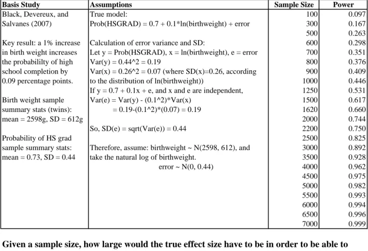
Given that there are relatively few data sets with information about early childhood influences and future outcomes, economists may be tempted to make use of relatively small data sets that happen to have the requisite variables. Power calculations can be helpful in determining ex ante whether analysis of a particular data set is likely to yield any interesting findings. Table 3 provides two sample calculations. The first half of the table considers the relationship between birth weight and future educational attainment as in Black et al. [2007]. Their key result was that a 1% increase in birth weight increased high school completion by .09 percentage points. The example shows that under reasonable assumptions about the distribution of birth weight and schooling attainment, it requires a sample of about 4000 children to be able to detect this effect in an OLS regression. We can also turn the question around and ask, given a sample of a certain size, how large would an effect have to be before we could be reasonably certain of finding it in our data? The second half of the table shows that if we were looking for an effect of birth weight on a particular outcome in a sample of 1,300 children, the coefficient on (the log of ) birth weight would have to be at least .15 before we could detect it with reasonable confidence. If we have reason to believe that the effect is smaller, then it is not likely to be useful to estimate the model without more data.

3.2

Data Constraints

The lack of large-scale longitudinal data (i.e. data that follows the same persons over time) has been a frequent obstacle to evaluating the long-term impacts of early life influences. Nevertheless, the answer may not always be to undertake collection of new longitudinal data. Drawbacks include the high costs of data collection; the fact that long term outcomes cannot be assessed for some time; and the fact that limiting sample attrition is particularly costly. Unchecked, attrition in longitudinal data can pose challenges for inference.

3.2.1 Leveraging Existing Datasets

In many cases, existing cross-sectional microdata can serve as a platform for constructing longitudinal datasets. First, it may be possible to add retrospective questions to ongoing data collections. Second, it may be possible to merge new group-level information to existing data sets. Third, it may be possible to merge administrative data sets by individual in order to address previously unanswerable questions. The primary obstacle to implementing each of these data strategies is frequently data security. Depending on the approach adopted, there are different demands on data security, as described below. Smith [2009] and Garces et al. [2002] are examples of adding retrospective questions to existing data collections. Smith had retrospective questions about health in childhood added to the Panel Study of Income Dynamics (PSID). The PSID began in the 1960s with a representative national sample, and has followed the original respondents and their family members every since. Using these data, Smith [2009] is able to show that adult respondents who were in poor health during childhood have lower earnings than their own siblings who were not in poor health. Such comparisons are possible because the PSID has data on large numbers of sibling pairs. Garces et al. [2002] added retrospective questions about Head Start participation to the PSID, and were able to show that young adults who had attended Head Start had higher educational attainment, and were less likely to have been booked or charged with a crime than siblings who had not attended. While these approaches may enable analyses of long-term impacts even in the ab-sence of suitable “off the shelf” longitudinal data, they have their drawbacks. First, retrospective data may be reported with error, although it may be possible to assess the extent of reporting error using data from other sources. Second, only outcomes that are already in the data can be assessed, so the need for serendipity remains. Still, the method is promising enough to suggest that on-going, government funded data col-lections should build-in mechanisms whereby researchers can propose the addition of

questions to subsequent waves of the survey.

A second way to address long-term questions is to merge new information at the group level to existing data sets. The merge generally requires the use of geocoded data. For some purposes, such as exploring variations in policies across states, only a state identifier is required. For other purposes, such as examining the effects of traffic patterns on asthma, ideally the researcher would have access to exact latitude and longitude. There are many examples in which this approach has been successfully employed. For example, Ludwig and Miller [2007] study the long term effects of Head Start which exploits the fact that the Office of Economic Opportunity initially offered the 300 poorest counties in the country assistance in applying for Head Start. They show, using data from the National Educational Longitudinal Surveys, that children who were in counties just poor enough to be eligible for assistance were much more likely to have attended Head Start than children in counties that were just ineligible. They go on to show that child mortality rates in the relevant age ranges were lower in counties whose Head Start enrollments were higher due to the OEO assistance. Using Census data they find that education is higher for people living in areas with higher former Head Start enrollment rates. Unfortunately, however, neither the decennial Census nor the American Community Survey collect county of birth, so they cannot identify people who were born in these counties (substantial measurement error is obviously introduced by using county of residence or county where someone went to school as a proxy for county of birth). An exciting crop of new research would be enabled by the addition of Census survey questions on county of birth, as well as county of residence at key developmental ages (e.g., ages 5 and 14).9

In addition to the observational approaches described above, an intriguing possibility is that participants in a completed randomized trial could be followed up. For instance, Rush, Stein, and Susser [1980] conducted a randomized intervention of a prenatal nu-trition program in Harlem during the early 1970s. Following these children over time would allow researchers to evaluate cognitive outcomes in secondary school, and it might be possible to collect retrospective data on parental investments during childhood, and to evaluate whether parental investments were affected by the randomization.

9_{In another example, Currie and Gruber [1996b] were able to examine the effects of the Medicaid} expansions on the utilization of care among children by merging state-level information on Medicaid policy to data from the National Health Interview Survey (NHIS). At the time, this was only possible because one of the authors had access to the NHIS state codes through his work at the Treasury De-partment. It has since become easier to access geocoded health data either by travelling to Washington to work with the data, or by using it in one of the secure data centers that Census and the National Centers for Healh Statistics (NHCS) support. However, it remains a source of frustration to health researchers that NCHS does not make state codes and/or codes for large counties available on its public use data sets.

A third approach to leveraging existing data merges administrative records from multiple sources at the individual level, which obviously requires personal identifiers such as names and birth dates or social security numbers. Access to such identifiers is especially sensitive. Nevertheless, it constitutes a powerful way to address many questions of interest. Several important studies have successfully exploited this approach outside of the US. For example, Sandra E. Black and Salvanes [2005], Black et al. [2007] use Norwegian data on all twins born over 30 years to look at long-term effects of birth weight, birth order, and family size on educational attainment. Currie, Stabile, Manivong, and Roos (forthcoming) use Canadian data on siblings to examine the effects of health shocks in childhood on future educational attainment and welfare use. Almond, Edlund, and Palme [2009] use Swedish data to look at the long term effects of low-level radiation exposure from the Chernobyl disaster on children’s educational attainment.

In the U.S., Doyle [2008] uses administrative data from child protective services and the criminal justice system in Illinois to examine the effects of foster care. He shows first that there is considerable variation between foster care case workers in whether or not a child will be sent to foster care. Moreover, whether a child is assigned to a particular worker is random, depending on who is on duty at the time a call is received. Using this variation, Doyle shows that the marginal child assigned to foster care is significantly more likely to be incarcerated in future. These examples exploit large sample sizes, objective indicators of outcomes, sibling or cohort comparisons, as well as a long follow up period. Some limitations of using existing data include the fact that administrative data sets often contain relatively little background information, and that outcomes are limited to those that are collected in the data bases. Finally, the application process to obtain individual-matched data is often protracted.

Looking forward, the major challenge to research that involves either merging new information to existing data sets, or merging administrative data sets to each other, is that privacy concerns are making it increasingly difficult to obtain data just as it is becoming more feasible to link them. In some cases, access to public use data has deteriorated. For example, for many years, individual level Vital Statistics Natality data from birth certificates included the state of birth, and the county (for counties with over 100,000 population). Since 2005, however, these data elements have been suppressed and it is now necessary to get special permission to obtain U.S. Vital Statistics data with geocodes.

3.2.2 Improvements in the Production of Administrative Data

There are several “first best” potential solutions to these problems. First, creators of large data sets need to be sensitive to the fact that their data may well be useful for addressing questions that they have not envisaged. In order to preserve the ability to use data to answer future questions, it is essential to retain information that can be used for linkage. At a minimum, this should include geographic identifiers at the smallest level of disaggregation that is feasible (for example a Census tract). Ideally, personal identifiers would also be preserved.

Second, more effort needs to be expended in order to make sensitive data available to researchers. A range of mechanisms exist that protect privacy while enabling research:

1. Suppress small cells or merge small cells in public use data files. For example, NCHS data sets such as NHIS could be released with state identifiers for large states, and with identifiers for groups of smaller states.

2. Add small amounts of “noise” to public use data sets, or do data swapping in order to prevent identification of outliers. For example, Cornell University is coor-dinating the NSF-Census Bureau Synthetic Data Project which seeks to develop public-use “analytically valid synthetic data” from micro datasets customarily ac-cessed at secure Census Research Data Centers.

3. Create model servers. In this approach, users login to estimate models using the true data, but get back output that does not allow individuals to be identified.

4. Data use agreements. The National Longitudinal Survey of Youth and the National Educational Longitudinal Survey have successfully employed data use agreements with qualified users for many years, and without any documented instances of data disclosure.

5. Creation of de-identified merged files. For example, Currie, Neidell, and Schmieder [2009a] asked the state of New Jersey to merge birth records with information about the location of pollution sources, and create a de-identified file. This allows them to study the effect of air pollution on infant health.

6. Secure data facilities. The Census Research Data Centers have facilitated access to much confidential data, although researchers who are not located close to the facilities may still face large costs of accessing them.

These approaches to data dissemination have been explored in the statistics literature for more than 20 years (see Dalenius and Reiss [1982], and have been much discussed at Census (see for example, Reznek [2007]).

3.2.3 Additional Issues

We conclude with two new and relatively unexplored data issues. First, how can economists make effective use of the burgeoning literature on biomarkers? These mea-sures have recently been added to existing health surveys, such as the National Longitu-dinal Study of Adolescent Health data. Biomarkers include not only information about genetic variations but also hormones such as cortisol (which is often interpreted as a measure of stress). It is tempting to think of these markers as potential instrumental variables [Fletcher and Lehrer, 2009]. For instance, if it was known that a particular gene was linked to alcoholism, then one might think of using the gene as an instrument for alcoholism. The potential pitfall in this approach is clear if we consider using something like skin color as an instrument in a human capital earnings function–clearly, skin color may predict educational attainment, but it may also have a direct effect on earnings. Just because a variable is “biological” does not mean that it satisfies the criteria for a valid instrument.

A second issue is the evolving nature of what constitutes a “birth cohort”. Improve-ments in neonatal medicine have meant that stillbirths and fetal deaths that would pre-viously have been excluded from the census of live births may be increasingly important, e.g. MacDorman, Martin, Mathews, Hoyert, and Ventura [2005]). Such a compositional effect on live births may have first order-implications for program evaluation and the long-term effects literature. Indeed, both the right and left tails of the birth weight distribution have elongated over time – in 1970 there were many fewer live births with birthweight either less than 1500 grams or over 4000 grams. To date there has been little research exploring the implications of these compositional changes.

In summary, there are many secrets currently locked in existing data that researchers do not have access to. Economists have been skillful in navigating the many data chal-lenges inherent in the analysis of long-term (and sometimes latent) effects. Nevertheless, we need to explore ways to make more of these data available, and to more researchers. In many cases, this will be a more cost effective and timely way to answer important questions than carrying out new data collections.

4

Empirical Literature: Evidence of Long Term

Con-sequences

What is of importance is the year of birth of the generation or group of in-dividuals under consideration. Each generation after the age of 5 years seems to carry along with it the same relative mortality throughout adult life, and even into extreme old age.

Kermack et al. [1934] in The Lancet (emphasis added).

In this section, we summarize recent empirical research findings that experiences before five have persistent effects, shaping human capital in particular. A hallmark of this work is the attention paid to identification strategies that seek to isolate causal effects of the early childhood environment. An intriguing sub-current is the possibility that some of these effects may remain latent during childhood (at least from the researcher’s perspective) until manifested in either adolescence or adulthood. Recently, economists have begun to ask how parents or other investors in human capital (e.g. school districts)

respond to early-life shocks, as suggested by the conceptual framework in Section 2.3. As the excerpt from Kermack et al. [1934] indicates, the idea that early childhood experiences may have important, persistent effects did not originate recently, nor did it first appear in economics. An extensive epidemiological literature has focussed on the early childhood environment, nutrition in particular, and its relationship to health outcomes in adulthood. For a recent survey, see Gluckman and Hanson [2006]. This literature has been criticized within epidemiology for credulous empirical comparisons (see, e.g. Rasmussen [2001] or editorial inThe Lancet[2001]). Absent clearly-articulated identification strategies, health determinants that are difficult to observe and are there-fore omitted from the analysis (e.g., parental concern) are presumably correlated with the treatment and can thereby generate the semblance of “fetal origins” linkages, even when such effects do not exist.

4.1

Prenatal Environment

In the 1990s, David J Barker popularized and developed the argument that disruptions to the prenatal environment presage chronic health conditions in adulthood, including heart disease and diabetes [Barker, 1992]. Growth is most rapid prenatally and in early childhood. When growth is rapid, disruptions to development caused by the adverse environmental conditions may exert life-long health effects. Barker’s “fetal origins”

perspective contrasted with the view that pregnant mothers functioned as an effective buffer for the fetus against environmental insults.10

In Table 4, we categorize prenatal environmental exposures into three groups. Specif-ically, we differentiate among factors affecting maternal and thereby fetal health (e.g. nutrition and infection), economic shocks (e.g. recessions), and pollution (e.g. ambient lead).

4.1.1 Maternal Health

Currie and Hyson [1999] broke ground in economics by exploring whether “fetal origins” (FO) effects were confined to chronic health conditions in adulthood, or might extend to human capital measures. Using the British National Child Development Survey, low birth weight children were more than 25% less likely to pass English and math O-level tests, and were also less likely to be employed. The finding that test scores were substan-tially affected was surprising as epidemiologists routinely posited fetal “brain sparing” mechanisms, whereby adversein uteroconditions were parried through a placental triage that prioritized neural development over the body, see, e.g., Scherjon et al. [1996]. Fur-thermore, Stein et al. [1975]’s influential study found no effect of prenatal exposure to the Dutch Hunger Winter on IQ.

Currie and Hyson [1999] were followed by a series of papers that exploited differ-ences in birthweight among siblings and explored their relationship to sibling differdiffer-ences in completed schooling. In relatively small samples (approximately 800 families), Conley and Bennett [2001] found negative but imprecise effects of low birth weight on educa-tional attainment. Statistically significant effects of low birth weight on educaeduca-tional attainment were found when birth weight was interacted with being poor, but in general sample size prevented detection of all but the largest effects (see Section 3.1). Using a comparable sample size, Behrman and Rosenzweig [2004] found the schooling of identical female twins was nearly one-third of a year longer for a pound increase in birth weight (454 grams), with relatively imprecise effects on adult BMI or wages.

In light of the above power concerns, Currie and Moretti [2007] matched mothers to their sisters in half a million birth records from California. Here, low birth weight was found to have statistically significant negative impacts on educational attainment and the likelihood of living in a wealthy neighborhood. However, the estimated magnitudes of the main effects were more modest: low birth weight increased the likelihood of living in a poor neighborhood by 3% and reduced educational attainment approximately one month 10_{For example, it has been argued that nausea and vomiting in early pregnancy (morning sickness)} is an adaptive response to prevent maternal ingestion of foods that might be noxious to the fetus.

on average. Like Conley and Bennett [2001], the relationship was substantially stronger for the interaction between low birth weight and being born in poor neighborhoods.

In a sample of Norwegian twins, Black, Devereux, and Salvanes [2007] also found long-term effects of birth weight, but did not detect any heterogeneity in the strength of this relationship by parental socioeconomic status.11 _{Oreopoulos et al. [2008] find} similar results for Canada and Lin and Liu [2009] find positive long term effects of birth weight in Taiwan. Royer [2009] found long-term health and educational effects within California twin pairs, with a weaker effect of birth weight than several other studies, esp. Black, Devereux, and Salvanes [2007]. Responsive investments could account for this discrepancy if they differed between California and elsewhere (within twin pairs). Alternatively, there may be more homogeneity with respect to socioeconomic status in Scandanavia than in California. As described in Section 3, Royer [2009] analyzed invest-ment measures directly with the ECLS-B data, concluding that there was no evidence of compensatory or reinforcing investments (see Section 2.2).

Following a literature in demography on seasonal health effects, Doblhammer and Vaupel [2001] and Costa and Lahey [2005] focused on the potential long-term health effects of birth season. A common finding is that in the northern hemisphere, people born in the last quarter of the year have longer life expectancies than those born in the second quarter. Both the availability of nutrients can vary seasonally (particularly historically), as does the likelihood of common infections (e.g., pneumonia). Therefore, either nutrition or infection could drive this observed pattern. Almond [2006] focused on prenatal exposure to the 1918 Influenza Pandemic, estimating that children of in-fected mothers were 15% less likely to graduate high school and wages were between 5 and 9% lower. Kelly [2009] found negative effects of prenatal exposure to 1957 “Asian flu” in Britain on test scores, though the estimated magnitudes were relatively modest. Interestingly, while birth weight was reduced by flu exposure, this effect appears to be independent of the test score effect. Finally, Field, Robles, and Torero [2009] found that prenatal iodine supplementation raised educational attainment in Tanzania by half a year of schooling, with larger impacts for girls.

4.1.2 Economic Shocks

A second set of papers considers economic shocks around the time of birth. Here, health in adulthood tends to be the focus (not human capital), and findings are perhaps less consistent than in the studies of nutrition and infection described above. Berg et al. 11_{Royer [2009] notes that Black, Devereux, and Salvanes [2007] find a “negligible effect of birth weight} on high school completion for the 1967-1976 birth cohort, but for individuals born between 1977 and 1986, the estimate is nearly six times as large.”

[2006]’s basic result is that adult survival in the Netherlands is reduced for those born during economic downturns. In contrast, Cutler et al. [2007] detected no long term morbidity effects in the Health and Retirement Survey data for cohorts born during the Dustbowl era of 1930s. Banerjee, Duflo, Postel-Vinay, and Watts [2009] found that shocks to the productive capacity of French vineyards did not have detectable effects on life expectancy or health outcomes, but did reduce height in adulthood. Baten, Crayen, and Voth [2007] related variations in grain prices in the decade of birth to numeracy using an ingenious measure based on “age heaping” in the British Censuses between 1851 and 1881. Persons who are more numerate are less likely to round their ages to multiples of 5 or 10. They find that children born in decades with high grain prices were less numerate by this index.

4.1.3 Air Pollution

The third strand of the literature examines the effect of pollution on fetal health. Epi-demiological studies have demonstrated links between very severe pollution episodes and mortality: one of the most famous focused on a “killer fog” in London, England and found dramatic increases in cardiopulmonary mortality [Logan and Glasg, 1953]. Pre-vious epidemiological research on the effects of moderate pollution levels on prenatal health suggests negative effects but have produced inconsistent results. Cross-sectional differences in ambient pollution are usually correlated with other determinants of fetal health, perhaps more systematically than with nutritional or disease exposures consid-ered above. Many of the pollution studies have minimal (if any) controls for these potential confounders. Banzhaf and Walsh [2008] found that high-income families move out of polluted areas, while poor people in-migrate. These two groups are also likely to provide differing levels of (non-pollution) investments in their children, so that fetuses and infants exposed to lower levels of pollution may tend to receive, e.g., better quality prenatal care. If these factors are unaccounted for, this would lead to an upward bias in estimates. Alternatively, certain pollution emissions tend to be concentrated in urban areas, and individuals in urban areas may be more educated and have better access to health care, factors that may improve health. Omitting these factors would lead to a downward bias, suggesting the overall direction of bias from confounding is unclear.

Two studies by Chay and Greenstone [2003b,a] address the problem of omitted con-founders by focusing on “natural experiments” provided by the implementation of the Clean Air Act of 1970 and the recession of the early 1980s. Both the Clean Air Act and the recession induced sharper reductions in particulates in some counties than in others, and they use this exogenous variation in levels of pollution at the county-year level to

identify its effects. They estimate that a one unit decline in particulates caused by the implementation of the Clean Air Act (recession) led to between five and eight (four and seven) fewer infant deaths per 100,000 live births. They also find some evidence that the decline in Total Suspended Particles (TSPs) led to reductions in the incidence of low birth weight. However, only TSPs were measured at that time, so that they could not study the effects of other pollutants. And the levels of particulates studied by Chay and Greenstone are much higher than those prevalent today; for example, PM10 (particulate matter of 10 microns or less) levels have fallen by nearly 50 percent from 1980 to 2000. Several recent studies consider natural experiments at more recently-encountered pollution levels. For example, Currie, Neidell, and Schmieder [2009a] use data from birth certificates in New Jersey in which they know the exact location of the mothers residence, and births to the same mother can be linked. They focus on a sample of mothers who live near pollution monitors and show that variations in pollution from carbon monoxide (which comes largely from vehicle exhaust) reduces birth weight and gestation. Currie and Walker [2009] exploit a natural experiment having to do with introduction of electronic toll collection devices (E-ZPass) in New Jersey and Pennsylvania. Since much of the pollution produced by automobiles occurs when idling or accelerating back to highway speed, electronic toll collection greatly reduces auto emissions in the vicinity of a toll plaza. Currie and Walker [2009] compare mothers near toll plazas to those who live near busy roadways but further from toll plazas and find that E-ZPass increased birth weight and gestation. They show that they obtain similar estimates following mothers over time and estimating mother fixed effects models. These papers are notable in part because it has proven more difficult to demonstrate effects of pollution on fetal health than on infant health, as discussed further below. Hence, it appears that beingin utero

may be protective against at some forms of toxic exposure (such as particulates) but not others.

This literature on the effects of air pollution is closely related to that on smoking. Smoking is, afterall, the most important source of indoor air pollution. Medical research has shown that nicotine constricts the oxygen supply to the fetus, so there is an obvious mechanism for smoking to affect infant health. Indeed, there is near unanimity in the medical literature that smoking is the most important preventable cause of low birth weight. Economists have focussed on ways to address heterogeneity in other determi-nants of birth outcomes that is likely associated with smoking. Tominey [2007] found that relative to a conventional multivariate control specification, roughly one-third of the harm from smoking to birth weight is explained by unobservable traits of the mother. Moreover, the reduction in birth weight from smoking was substantially larger for

low-SES mothers. In a much larger sample, Currie, Neidell, and Schmieder [2009a] showed that smoking significantly reduced birth weight, even when comparisons are restricted to within-sibling differences. Moreover, Currie, Neidell, and Schmieder [2009a] document a significant interaction effect between exposure to carbon monoxide exposure and infant health in the production of low birth weight, which may help explain the heterogeneity in birth weight effects reported by Tominey [2007]. Aizer and Stroud [2009] note that impacts of smoking on birth weight are generally much smaller in sibling comparisons than in OLS and matching-based estimates. Positing that attenuation bias is accentu-ated in the sibling comparisons, Aizer and Stroud [2009] use serum cotinine levels as an instrument for measurement error in smoking and find that sibling comparisons yield similar birth weight impacts (around 150 grams). Lien and Evans [2005] use increases in state excise taxes as an instrument for smoking and find large effects of smoking on birth weight (182 grams) as a result. Using propensity score matching, Almond, Chay, and Lee [2005] document a large decrease in birth weight from prenatal smoking (203 grams), but argue that this weight decrease is weakly associated with alternative measures of infant health, such as prematurity, APGAR score, ventilator use, and infant mortality.

Some recently-released data will enable new research on smoking’s short and long-term effects. In 2005, twelve states began using the new U.S. Standard Certificate of Live Birth (2003 revision). Along with other new data elements (e.g., on surfactant replacement therapy), smoking behavior is reported by trimester. It will be useful to consider whether smoking’s impact on birth weight varies by trimester, and also whether smoking is more closely tied to other measures of newborn health if it occurs early versus late in pregnancy. Second, there is relatively little research by economists on the long-term effects of prenatal exposure to smoking. Between 1990 and 2003, there were 113 increases in state excise taxes on cigarettes [Lien and Evans, 2005].12 Since 2005, the American Community Survey records both state and quarter of birth, permitting linkage of these data to the changes in state excise taxes during pregnancy.

Almond, Edlund, and Palme [2009] examine the effect of pollution from the Cher-nobyl disaster on the Swedish cohort that wasin utero at the time of the disaster. Since the path of the radiation was very well measured, they can compare affected children to those who were not affected as well as to those born in the affected areas just prior to the disaster. They find that in the affected cohort those who suffered the greatest radiation exposure were 3 percent less likely to qualify for high school, and had 6% lower math grades (the measure closest to IQ). The estimated effects were much larger 12_{Some states enacted earlier excise taxes: the “average state tax rate increased from 5.7 cents in 1964} to 15.5 cents in 1984” [Farrelly, Nimsch, and James, 2003]; high 1970s inflation can be an additional potential source of identification as excise taxes were set nominally.

within families. A possible interpretation is that cognitive damage from Chernobyl was reinforced by parents.

To summarize, the recent “fetal origins” literature in economics finds substantial effects of prenatal health on subsequent human capital and health. As we discuss in Section 5, this suggests a positive role for policies that improve human capital by affect-ing the birth endowment. That is, despite beaffect-ing congenital (i.e. present from birth), this research indicates that the birth endowment is malleable in ways that shape hu-man capital. This finding has potentially radical implications for public policy since it suggests that one of the more effective ways to improve children’s long term outcomes might be to target women of child bearing age in addition to focusing on children after birth.

4.2

Early Childhood Environment

It would be surprising to find that a very severe shock in early childhood (e.g., a head injury, or emotional trauma) had no effect on an individual. Therefore, a more interest-ing question from the point of view of research is how developmental linkages operatinterest-ing at the individual level affect human capital formation in the aggregate. To answer this question, we need to know how many children are affected by negative early childhood experiences that could plausibly exert persistent effects? How big and long-lasting are the effects of less severe early childhood shocks relative to more severe shocks? Taken together, how much of the differences in adult attainments might be accounted for by things that happen to children between birth and age five? Furthermore, how are these linkages between shocks and outcomes mediated or moderated by third factors? For example, is the effect of childhood lead exposure on subsequent test scores stronger for families of lower socioeconomic status (i.e. is the interaction with SES an important one) and if so why? Alternatively, is the effect of injury mediated by health status, or is the causal pathway a direct one to cognition?

We might also wish to know how parents respond to early childhood shocks. To date, there has been less focus on this question in the early childhood period than in the prenatal period, perhaps because it seems less plausible to hope to uncover a “pure” biological effect of a childhood shock given that children are embedded in families and in society. However, this embeddedness opens the possibility that a richer set of behavioral responses – of the kind considered by economists – might be at play. Furthermore, early childhood admits a wider set of environmental influences than the prenatal period. For example, abuse in early childhood can be distinguished from malnutrition, a distinction more difficult for the in utero period, and these may have quite different effects.

We define early childhood as starting at birth and ending at age five. From an empirical standpoint, early childhood so defined offers advantages and disadvantages over analyses that focus on the prenatal period. Mortality is substantially lower during early childhood than in utero, which reduces the scope for selective attrition caused by environmental shocks to affect the composition of survivors. On the other hand, it is unlikely that environmental sensitivity during early childhood tapers discontinuously at any precise age (including age five). From a refutability perspective, we cannot make sharp temporal comparisons of a cohort “just exposed” to a shock during early childhood to a neighboring cohort “just unexposed” by virtue of its being too old to be sensitive. Moreover, it will often be difficult to know a priori whether prenatal or postnatal expo-sure is more influential.13 _{Thus, studies of early childhood exposures tend to emphasize} cross-sectional sources of variation, including that at the geographic and individual level. The studies reviewed in this section focus on tracing out the relationships between events in early childhood and future outcomes, and are summarized in Table 5.

4.2.1 Infections

Insofar a specific health shocks are considered, infections are the most commonly studied. In epidemiology, long-term health effects of infections – and the inflammation response they trigger – has been explored extensively, e.g. Crimmins and Finch [2006]. Out-comes analyzed by economists include height, health status, educational attainment, test scores, and labor market outcomes. The estimated impacts tend to be large. Using geographic differences in hookworm infection rates across the US South, Bleakley [2007] found that eradication after 1910 increased literacy rates but did not increase the amount of completed schooling, except for Black children. The literacy improvement was much larger among Blacks than Whites, and stronger among women then men. The return to education increased substantially, and Bleakley [2007] estimated that hookworm infec-tion throughout childhood reduced wages in adulthood by as much as 40%. Case and Paxson [2009] focussed on reductions in U.S. childhood mortality from typhoid, malaria, measles, influenza, and diarrhea during the first half of the 20th Century. They found that improvements in the disease environment in one’s state of birth were mirrored by improved cognitive performance at older ages, but like Bleakley [2007], this effect did not seem to operate through increased years of schooling. However, the estimated cognitive impacts in Case and Paxson [2009] were not robust to the inclusion of state-specific time trends in their models.

13_{For example, early postnatal exposure to Pandemic influenza apparently had a larger impact on} hearing than did prenatal flu exposure [Heider, 1934].