Combining disaggregate forecasts or combining disaggregate information to forecast an aggregate

Working PaPer SerieS

no 1155 / FeBrUarY 2010

ComBining

diSaggregate

ForeCaStS or

ComBining

diSaggregate

inFormation

to ForeCaSt

an aggregate

W O R K I N G PA P E R S E R I E S

N O 115 5 / F E B R U A R Y 2 010

This paper can be downloaded without charge from http://www.ecb.europa.eu or from the Social Science Research Network electronic library at http://ssrn.com/abstract_id=1551223

In 2010 all ECB publications feature a motif taken from the €500 banknote.

COMBINING DISAGGREGATE

FORECASTS OR COMBINING

DISAGGREGATE INFORMATION

TO FORECAST AN AGGREGATE

by David F. Hendry

© European Central Bank, 2010 Address

Kaiserstrasse 29

60311 Frankfurt am Main, Germany Postal address

Postfach 16 03 19

60066 Frankfurt am Main, Germany Telephone +49 69 1344 0 Website http://www.ecb.europa.eu Fax +49 69 1344 6000

All rights reserved.

Any reproduction, publication and reprint in the form of a different publication, whether printed or produced electronically, in whole or in part, is permitted only with the explicit written authorisation of the ECB or the author(s).

The views expressed in this paper do not necessarily refl ect those of the European Central Bank.

Abstract 4 Non-technical summary 5 1 Introduction 7 2 Combining disaggregate forecasts or

disaggregate information 9 2.1 Combining disaggregate forecasts: new

analytical results 10 2.2 Forecasting the aggregate directly

by its past 12 2.3 Comparing aggregated disaggregate

versus aggregate forecast errors 13 2.4 Combining disaggregate information to

forecast the aggregate: variable selection or dimension reduction 15 3 Monte Carlo simulations 16 3.1 Simulation design 16 3.2 Simulation results 18 4 Forecasting aggregate US infl ation 21

4.1 Data 21

4.2 Combining disaggregate forecasts or disaggregate variables: AR and

VAR models 22 4.3 Disaggregate information in dynamic

factor models 25 4.4 Summary of empirical results 27 5 Conclusions 27

Appendix 28

References 29

Abstract

To forecast an aggregate, we propose adding disaggregate variables, instead of combining forecasts of those disaggregates or forecasting by a univariate aggregate model. New analytical results show the effects of changing coefficients, mis-specification, estimation uncertainty and mis-measurement error. Forecast-origin shifts in parameters affect absolute, but not relative, forecast accuracies; mis-specification and es-timation uncertainty induce forecast-error differences, which variable-selection procedures or dimension reductions can mitigate. In Monte Carlo simulations, different stochastic structures and interdependen-cies between disaggregates imply that including disaggregate information in the aggregate model improves forecast accuracy. Our theoretical predictions and simulations are corroborated when forecasting aggregate US inflation pre- and post 1984 using disaggregate sectoral data.

JEL: C51, C53, E31

Forecasts of macroeconomic aggregates are employed by the private sector, governmental and in-ternational institutions as well as central banks. There has been renewed interest in the effect of contemporaneous aggregation in forecasting, and the potential improvements in forecast accuracy by forecasting the component indices and aggregating such forecasts, over simply forecasting the ag-gregate itself.

attention by staff at central banks in the Eurosystem. Similarly, for short-term inflation forecasting, staff at the Federal Reserve Board forecast disaggregate price categories.

gate variables separately and aggregating those forecasts. In this paper, we suggest an alternative use of disaggregate information to forecast the aggregate variable of interest, namely including disaggre-gate variables in the model for the aggredisaggre-gate. An alternative to including disaggredisaggre-gate variables in the aggregate model might be to combine the information in the disaggregate variables first, then include the disaggregate information in the aggregate model. This entails a dimension reduction, potentially leading to reduced estimation uncertainty and reduced mean square forecast error. We include an example in our empirical analysis. A third alternative is to forecast the aggregate only using lagged aggregate information. Our analysis is relevant for policy makers and observers interested in inflation forecasts, since disaggregate inflation rates across sectors and regions are often monitored and used to forecast aggregate inflation. Many other applications of our results are possible, including forecast-ing other macroeconomic aggregates such as GDP growth, monetary aggregates or trade, since our assumptions in a large part of the analysis are fairly general. Our analysis extends previous literature in a number of directions outlined in the following.

First, our proposal of combining disaggregate information by including all, or a selected number of, disaggregate variables in the aggregate model is investigating the predictability content of disag-gregates for the aggregate from a new perspective. Most previous literature focused on combining disaggregate forecasts rather than disaggregate information.

Second, we present new analytical results for the forecast accuracy comparison of different uses of disaggregate information to forecast the aggregate, i.e. (1) combining disaggregate forecasts (fore-casting the disaggregate variables then aggregating those forecasts), (2) using only lagged aggregate information, and (3) to combine disaggregate information by including a subset of disaggregate com-ponents (or a combination thereof) in the aggregate model. In contrast to Hendry & Hubrich (2006) focusing on the predictability of the aggregate in population, we investigate the improvement in fore-cast accuracy related to the sample information. From the analytical comparisons of the forefore-cast The aggregation of forecasts of disaggregate inflation components is also receiving

The theoretical econometric literature has so far mainly been concerned with forecasting

error decompositions of the three different methods for forecasting an aggregate, we draw important conclusions regarding the effects of specification, estimation uncertainty, forecast origin mis-measurement, structural breaks and innovation errors for their relative forecast accuracy. Instabili-ties have generally been found important for the forecast accuracy of different forecasting methods. Therefore, an important extension of the previous literature on contemporaneous aggregation and forecasting is to allow for a DGP with an unknown break in the parameters and time-varying aggre-gation weights.

The decompositions of the sources of forecast errors led us to conclude that relative forecast accu-racy is not affected by forecast-origin location shifts and slope changes, whereas absolute accuaccu-racy is. This is in contrast to the usual forecast combination literature, which focuses on combining forecasts of the same variable, where combination helps in the presence of mean shifts in opposite directions. Our second main result, in addition to a number of other important conclusions, is that slope mis-specification and estimation uncertainty are the primary sources of differences in forecast accuracy between the different methods.

Third, we investigate by Monte Carlo simulations the effect of the stochastic structure of disag-gregates and their interdependencies, as well as structural breaks, estimation uncertainty and mis-specification, on the relative forecast accuracy of the different approaches to forecast the aggregate. We find that including disaggregate variables in the aggregate model helps forecast the aggregate if the disaggregates follow different stochastic structures, the components are interdependent, and only a selected number of components is included to reduce estimation uncertainty. Unknown and un-modeled structural change in the mean does not affect relative forecast error of the different forecast methods, even though it has major effects on absolute forecast accuracy.

Fourth, we examine whether our theoretical predictions can explain our empirical findings for the relative forecast accuracy of combining disaggregate sectoral information versus disaggregate fore-casts or just using past aggregate information to forecast aggregate US inflation. The empirical results for US CPI inflation before and after the Great Moderation confirmed our analytical and simulation findings that estimation uncertainty plays an important role in relative forecast accuracy across the different approaches to forecast an aggregate. Consequently, we recommend model selection proce-dures for choosing the disaggregates to be included in the aggregate model, or methods to combine disaggregate information as in factor models, and careful modeling of location shifts. Alternative methods for reducing estimation uncertainty are an interesting direction of further research in this context.

1

Introduction

Forecasts of macroeconomic aggregates are employed by the private sector, governmental and in-ternational institutions as well as central banks. There has been renewed interest in the effect of contemporaneous aggregation in forecasting, and the potential improvements in forecast accuracy by forecasting the component indices and aggregating such forecasts, over simply forecasting the aggre-gate itself (see e.g. Fair & Shiller (1990) for a related analysis for US GNP; Zellner & Tobias (2000) for industrialised countries’ GDP growth; Marcellino, Stock & Watson (2003) for disaggregation across Euro area countries; and Espasa, Senra & Albacete (2002) and Hubrich (2005) for forecasting euro area inflation.) The aggregation of forecasts of disaggregate inflation components is also receiv-ing attention by staff at central banks in the Eurosystem (see e.g. Benalal, Diaz del Hoyo, Landau, Roma & Skudelny (2004), Reijer & Vlaar (2006), Bruneau, De Bandt, Flageollet & Michaux (2007) and Moser, Rumler & Scharler (2007)). Similarly, for short-term inflation forecasting, staff at the Federal Reserve Board forecast disaggregate price categories (see e.g. Bernanke (2007)).

The theoretical literature shows that aggregating component forecasts is at least as accurate as directly forecasting the aggregate when the data generating process (DGP) is known, and lowers the mean squared forecast error (MSFE), except under certain conditions. If the DGP is not known and the model has to be estimated, the properties of the unknown DGP determine whether combining dis-aggregate forecasts improves the accuracy of the dis-aggregate forecast. It might be preferable to forecast the aggregate directly. Contributions to the theoretical literature on aggregation versus disaggrega-tion in forecasting can be found in e.g. Grunfeld & Griliches (1960), Kohn (1982), L¨utkepohl (1984, 1987), Granger (1987), Pesaran, Pierse & Kumar (1989), Garderen, Lee & Pesaran (2000), Giacomini & Granger (2004); see L¨utkepohl (2006) for a recent review on aggregation and forecasting. Since in practice the DGP is not known, it is largely an empirical question whether aggregating forecasts of disaggregates improves forecast accuracy of the aggregate of interest. Hubrich (2005), for example, shows that aggregating forecasts by component does not necessarily help to forecast year-on-year Eurozone inflation one year ahead.

In this paper, we suggest an alternative use of disaggregate information to forecast the aggregate variable of interest, namely including disaggregate variables in the model for the aggregate. This is distinct from forecasting the disaggregate variables separately and aggregating those forecasts, usually considered in previous literature. An alternative to including disaggregate variables in the aggregate model might be to combine the information in the disaggregate variables first, then include the disag-gregate information in the agdisag-gregate model. This entails a dimension reduction, potentially leading to reduced estimation uncertainty and reduced MSFE. Bayesian shrinkage methods or factor models

can be used for that purpose. We include the latter in our empirical analysis. A third alternative is to forecast the aggregate only using lagged aggregate information. Our analysis is relevant for policy makers and observers interested in inflation forecasts, since disaggregate inflation rates across sectors and regions are often monitored and used to forecast aggregate inflation. Many other applications of our results are possible, including forecasting other macroeconomic aggregates such as GDP growth, monetary aggregates or trade, since our assumptions in a large part of the analysis are fairly general. Our analysis extends previous literature in a number of directions outlined in the following.

First, our proposal of combining disaggregate information by including all, or a selected num-ber of, disaggregate variables in the aggregate model is investigating the predictability content of disaggregates for the aggregate from a new perspective. Most previous literature focused on combin-ing disaggregate forecasts rather than disaggregate information. Second, we present new analytical results for the forecast accuracy comparison of different uses of disaggregate information to fore-cast the aggregate. In contrast to Hendry & Hubrich (2006) focusing on the predictability of the aggregate in population, we investigate the improvement in forecast accuracy related to the sample information. From the analytical comparisons of the forecast error decompositions of the three dif-ferent methods for forecasting an aggregate, we draw important conclusions regarding the effects of mis-specification, estimation uncertainty, forecast origin mis-measurement, structural breaks and in-novation errors for their relative forecast accuracy. Instabilities have generally been found important for the forecast accuracy of different forecasting methods, see e.g. Stock & Watson (1996, 2007), Clements & Hendry (1998, 1999, 2006) and Clark & McCracken (2006). Therefore, an important extension of the previous literature on contemporaneous aggregation and forecasting is to allow for a DGP with an unknown break in the parameters and time-varying aggregation weights. Third, we investigate by Monte Carlo simulations the effect of the stochastic structure of disaggregates and their interdependencies, as well as structural breaks, estimation uncertainty and mis-specification, on the relative forecast accuracy of the different approaches to forecast the aggregate. Fourth, we examine whether our theoretical predictions can explain our empirical findings for the relative forecast accu-racy of combining disaggregate sectoral information versus disaggregate forecasts or just using past aggregate information to forecast aggregate US inflation. Note, that all empirical and simulation re-sults discussed in the text of the current paper that are not presented explicitly in tables or graphs are available from the authors upon request.

The paper is organised as follows. In Section 2, we present new analytical results on the relative forecast accuracy of different approaches to forecast the aggregate. Section 3 presents Monte Carlo evidence. In Section 4, we investigate whether our analytical and simulation results are confirmed in a pseudo out-of-sample forecasting experiment for US CPI inflation. Section 5 concludes.

2

Combining disaggregate forecasts or disaggregate information

In Hendry & Hubrich (2006) we presented analytical results on predictability of aggregates using disaggregates, as a property in population. In the following analytical derivations, we allow the model and the DGP to differ and the parameters need to be estimated. First, we extend previous literature including L¨utkepohl (1984, b), Kohn (1982) and Giacomini & Granger (2004), by allowing for a structural break at the forecast origin and forecast origin uncertainties due to measurement errors. We assume that the break is not known to the forecaster who continues to use the previous forecast model based on in-sample information. It is of interest to know whether and how the relative forecast accuracy of different methods to forecast the aggregate is affected by an unmodeled structural break. Second, we compare our proposed approach of including and combining disaggregate information directly in the aggregate model with previous methods.

Relation to other literature on aggregation and forecasting. Allowing for estimation uncer-tainty introduces a trade-off between potential biases due to not specifying the fully disaggregated system, and increases in variance due to estimating an unnecessarily large number of parameters. Gi-acomini & Granger (2004) show that in the presence of estimation uncertainty, to aggregate forecasts from a space-time AR model is weakly more efficient than the aggregate of the forecasts from a VAR. They also show that if their poolability condition is satisfied, i.e. zero coefficients on all included com-ponents is not rejected, it is more efficient to forecast the aggregate directly. Hernandez-Murillo & Owyang (2006) provide an empirical investigation of the Giacomini & Granger (2004) methodology. The space-time AR model implies certain restrictions on the correlation structure of the disaggre-gates. In contrast, in our proposal the type of restrictions depends on the model used. For instance, in a VAR our suggestion implies to impose zero restrictions on the coefficients of the disagggregates in the aggregate equation. In contrast to the empirical approach implemented in Carson, Cenesizoglu & Parker (2007) and Zellner & Tobias (2000), who impose the parameters of all or most of the disag-gregates to be identical across the individual empirical models, we suggest imposing either zero re-strictions on disaggregate parameters in the aggregate model or imposing a factor structure, where the weights of the disaggregates in the factor maximize their explained variance. Granger (1980, 1987) considers correlations among the disaggregates due to a common factor. Granger (1987) suggests that the forecast of the aggregate is simply the factor component of the disaggregate expectations, so empirically-derived disaggregate models may miss important factors, and are therefore mis-specified. Our proposed approach extends this idea, formally investigating the effect of mis-specification, es-timation uncertainty, breaks, forecast-origin mis-measurement, innovation errors, changing weights and a changing error variance-covariance structure. Another approach, implicit in Carson et al. (2007)

and Zellner & Tobias (2000), and explicitly analyzed in Hubrich (2005), is to impose the same vari-able selection across individual disaggregate models. Hubrich (2005) finds that allowing for different model specifications for different disaggregates does not improve forecast accuracy of the aggregate for euro area inflation.

In the following, we presentnew analytical resultscomparing forecast errors when forecasting the aggregate is the objective, for: (a) combining disaggregate forecasts (Section 2.1); (b) only using past aggregate information (Section 2.2); important conclusions comparing the analytics from (a) and (b) (Section 2.3); and (c) combining disaggregate information (Section 2.4). Unless otherwise stated, the following assumptions hold in this section:

Assumptions: The DGP of the disaggregates is stationary in-sample, but is unknown and has to be estimated. We allow for estimation uncertainty and model mis-specification as well as structural change in the mean and slope parameters and measurement error at the forecast origin, unknown to the forecaster. We also allow for (unknown) changes in aggregation weights out-of-sample. Our analytical derivations analyse the effects of those assumptions on the forecast error for the different methods to forecast an aggregate.

Let yt denote the vector of n disaggregate price changes with elements yi,t. The DGP for the disaggregates is assumed to be anI(0) VAR with unknown parameters that are constant in-sample and have to be estimated:

yt=μ+Γyt₋₁+t for t = 1, . . . T (1) wheret ∼ID[0,Ω](ID: identically distributed), but with a break at the forecast originT when:

yT₊h =μ∗+Γ∗yT₊h₋₁+T₊h for h= 1, . . . H (2)

although the process stays I(0). This break is assumed to be unknown to the forecaster. Such a putative DGP reflects the prevalence of forecast failure in economics by its changing parameters. Let

ya

t =ωtytbe the aggregate price index with weightsωt, which is the variable of interest.

2.1

Combining disaggregate forecasts: New analytical results

We first construct a decomposition of all the sources of forecast errors from aggregating the disaggre-gate forecasts using an estimated version of (1) when the forecast period is determined by (2).

This analysis follows the VAR taxonomy in Clements & Hendry (1998), but we only consider 1-step forecasts although allowyT to be subject to forecast-origin measurement errors (multi-step ahead forecasts add further terms, which we omit for readibility). Section 2.2 provides the corresponding taxonomy for the forecast errors from forecasting the aggregate directly from its past. In both cases,

in-sample changes in the weights ωt make the analysis intractable, so we assume constant weights here, but refer to the implications of changing weights in Section 2.3. The weights are assumed to be positive and to lie in the interval[0,1].

First, for the aggregated disaggregate forecast, taking expectations in (1) under stationarity – if the DGP is integrated, it must be transformed to a stationary representation – yields:

E[yt] =μ+ΓE[yt₋₁] =μ+Γφy =φy,

which is the long-run mean,φ_y = (In−Γ)−1μ, referred to as the “equilibrium mean” by Clements & Hendry (1998, 2006) , as it is the value to which the process converges in the absence of further shocks. Nevertheless, the long-run mean might shift from a structural break. Further:

yt−E[yt] =yt−φy =Γ

yt₋₁−φy

+t. (3)

(3) represents the deviation of the disaggregates from their long-run mean, which will facilitate the decomposition of the forecast errors below, and isolate terms that only affect the bias.

The forecasts from the estimated disaggregate model (1) at the estimated forecast originyT are:

yT_+1|T =φy+Γ yT −φy (4) where fromT + 1onwards, the aggregated 1-step forecast errorsT_+1|T =yT₊₁−yT_+1|T are:

ω_T +1|T = ω_φ∗ y−ωφy +ω_Γ∗_{yT −φ}∗ y −ω_{ΓyT −φ} y +ω_T +1. (5)

Assuming the relevant moments exist, as is likely here, letE[Γ] =Γe andE[φy] =φy,e

The forecast-error taxonomy follows by decomposing each term in (5) into its components, namely, the parameter shifts, parameter mis-specifications, and the estimation uncertainty of the parameters. As the DGP is I(0), the dependence of the estimated parameters on the last observation isOp(T−1), as can be seen by terminating estimation atT −1, so is omitted below (in contrast, see Elliott (2007) for the case of a non-stationary DGP).

ω_{Γ(yT − yT) can be decomposed (see Appendix for details), yielding the taxonomy in (6).}

This forecast-error decomposition facilitates the analysis of the effects of structural change, model mis-specification, estimation uncertainty and forecast-origin mis-measurement, since specific terms involving these each vanish once no structural change, or a correctly specified model etc., is assumed. Terms with non-zero means only affect the bias of the forecast and are shown in bold.

Aggregated disaggregate forecast-error decomposition ω_T +1|T = ω_(In−Γ∗_)φ∗ y−φy

(ia)long-run mean change +ω_(Γ∗_{−Γ)yT −φ}

y

(ib) slope change

+ω_{(In−Γe)φy−φy,e (iia)long-run mean mis-specification}

+ω_{(Γ−Γe)yT −φ}

y

(iib) slope mis-specification

+ω_(In−Γe)φ

y,e−φy

(iiia) long-run mean estimation

−ω_{Γ−Γe yT −φ}

y,e

(iiib) slope estimation

−ω_{Γe(yT −yT) (iv)forecast-origin mis-measurement}

+ω_{Γ−Γe φy −φy,e (va) covariance interaction} −ω_{Γ−Γe(yT −yT) (vb) mis-measurement interaction}

+ω_T

+1 (vi) innovation error.

(6)

2.2

Forecasting the aggregate directly by its past

When forecasting the aggregate directly by its own past alone, and the weights are constant,ωt=ω, pre-multiply (1) byω to derive the aggregate relation:

ya t = ωφy +ωΓ yt₋₁−φy +ω_t = τ +κya t₋₁−τ +νt (7)

where, in the second line, τ = ωφy, yta₋₁ = ωyt₋₁, and(τ, κ)orthogonalize 1,(yta₋₁−ωφy)

with respect toνt. Hence:

νt=ω(Γ−κIn)yt₋₁−φy

+ω_{t (8)}

whereκ = ωQΓω/ωQω. E[(yt−φy)(yt−φy)] = QandQ = ΓQΓ+Ωis the standardized sample second-moment matrix (about means) of the disaggregatesyt.

The taxonomy of the sources of 1-step ahead forecast errors foryTa₊₁ for a forecast origin at T from (8) highlight the potential gains from adding disaggregates to (7). The forecast-period DGP is (2) andωφ∗_y =τ∗: ya T₊₁ =ωφ∗y+ωΓ∗ yT −φ∗y +ω_T +1, with: ya T_+1|T =τ+κ(yTa −τ)

wherey_Ta =ωyT, matching (4). LetνT_+1|T =yaT₊₁−yTa_+1|T, then in a similar notation to above:

νT_+1|T = (τ∗−τ) +ωΓ∗yT −φ∗y

−κ(ya

T −τ) +ωT₊₁. (9)

The derivations of the corresponding taxonomy are similar, leading to (10). Where it helps to under-stand the relationship to (6), we have rewritten terms likeτ∗ −τ asω(φ∗y −φy)which highlights the close similarities. Terms in bold letters again denote those that need not be zero under uncondi-tional expectations, but would be zero if no shift in the mean occurred over the forecast period when a well-specified model was used from accurate forecast-origin measurements.

Direct aggregate forecast-error decomposition

νT_+1|T =

ω_(In−Γ∗_)φ∗

y−φy

(Ia)long-run mean change +ω_(Γ∗_{−Γ)yT −φ}

y

(Ib) slope change

+ (1−κ) (τ −τe) (IIa)long-run mean mis-specification

+ω_{(Γ−κIn)yT −φ}

y

(IIb) slope mis-specification

+ (1−κ) (τe−τ) (IIIa) long-run mean estimation

+ (κ−κ)ω_{yT −φ}

y

(IIIb) slope estimation

−κω_{(yT −yT) (IV)forecast-origin mis-measurement} + (κ−κ) (τ−τ) (Va) covariance interaction + (κ−κ)ω_{(yT −yT) (Vb) mis-measurement interaction} +ω_T +1 (VI) innovation error. (10)

2.3

Comparing Aggregated Disaggregate versus Aggregate Forecast Errors

Seven important conclusions follow from comparing the forecast errors from combining disaggregate forecasts in equation (6), with forecast errors from forecasting the aggregate directly as in (10):

1. (Ia) is identical to (ia). This implies that unkown forecast-origin location shifts affect both methods of forecasting the aggregate in precisely the same way. This is an important and sur-prising result, since no matter how the long-run (or unconditional) means of the disaggregates shift, the two approaches suffer identically in terms of forecast accuracy. Therefore, relative forecast accuracy is not affected, while absolute forecast accuracyis affected. In contrast to previous literature on forecast combination of different forecast models for the same variable (see e.g. Clements & Hendry (2004)), there is no benefit in MSFE terms in the presence of un-known (and therefore unmodeled) forecast origin location shifts from combining disaggregate forecasts to forecast an aggregate.

2. Comparing (Ib) and (ib) shows that unknown slope changes at the forecast origin also do not af-fect the relative forecast accuracy of the different forecasting methods of the aggregate. There-fore, there are no gains or losses from aggregating disaggregates or directly forecasting the aggregate in the presence of all forms of unkown breaks at the forecast origin–this is arelative comparison, since both approaches can be greatlyaffected absolutelyby such breaks.

3. Long-run mean mis-specification in (IIa) and (iia) is unlikely in both taxonomies when the in-sample DGP is constant and the model is well specified.

4. The innovation error effects in (VI) and (vi) are also identical in population, irrespective of the covariance structure of the errors, and even if that were also to change at the forecast origin. 5. The impacts of forecast-origin mis-measurement in (iv) and (IV), namelyωΓe(yT −yT)

ver-sus κω(yT −yT), are primarily determined by the relative slope mis-specifications. In the empirical analysis in Section 4, we use factor models to deal with potential measurement er-rors.

6. The interaction terms (Va,Vb) and (va, vb) will be small due to the specification in terms of the long-run mean and its deviation therefrom. Therefore, the covariance interaction terms (Va) and (va) have zero mean. Also, terminating estimation at T −1at a cost ofOp(T−1)should induce a zero mean of the mis-measurement interaction terms (Vb) and (vb).

7. Thus, we conclude that slope mis-specification (IIb) and (iib) and estimation uncertainty ((IIIa, IIIb) and (iiia, iiib)) are the primary sources of forecast error differences between these two approaches to forecast an aggregate. Mean and slope mis-specification only affect the condi-tional expectations, and in practice depend on how close the aggregate model approximates the true DGP relative to the disaggregate model. Estimation uncertainty only affects the conditional variances and so depend on their respective data second moments (and hence on Ω). Thus, it is not possible to make general statements about whether differences in forecast accuracy are mainly due to the bias or variance of the forecast.

All our conclusions will remain true for small changes in the weightsωT over the forecast horizon. Changes of weights, or incorrect forecasts thereof,(ωT₊₁−ωT₊₁), are additional sources of error. We leave more detailed investigation of that issue for future research.

2.4

Combining disaggregate information to forecast the aggregate: Variable

selection or dimension reduction

An alternative to the two methods for forecasting an aggregate considered in the previous sections, is to include disaggregate variables in the aggregate model. Since the DGP for the disaggregates is (1), from (7) and (8): ya t = τ +ρ ya t₋₁−τ +ω_{(Γ−ρIn)yt} −1−φy +ω_t = τ +ρya t₋₁−τ + n₋₁ i₌₁ πiyi,t₋₁−φy,i +νt (11)

say, whereπ =ω(Γ−ρIn)andρis the resulting autoregressive coefficient. In (11), the aggregate

ya

t depends on lags of the aggregate, yta₋₁, and the lagged disaggregatesyi,t₋₁. Thus, if the DGP is (1) at the level of the components, an aggregate model could be systematically improved by adding disaggregates to the extent thatπi =0. This could be ascertained by anF-test. Here, (11) is correctly specified given (1), so dropping yt₋₁ would induce dynamic mis-specification whenπ = 0, but of-fer a trade-off of mis-specification versus estimation variation. If no disaggregates are included, so forecasting the aggregate by its past, the forecast error decomposition (10) applies. If all but one dis-aggregate variables are added to the dis-aggregate model, the combined disdis-aggregate model is recovered, so the forecast error taxonomy (6) applies. Our combination of disaggregate variables will inherit the common effects in Section 2.3, but will differ in terms of slope mis-specification and estimation uncertainty. Selection of a subset of the most relevant disaggregates to add to the model might help improve forecast accuracy of the aggregate, largely by reducing estimation uncertainty. The forecast accuracy improvement depends on the explanatory power of the disaggregates in anR2sense. Conse-quently, our proposal could dominate both previous alternatives depending on the relative importance of the disaggregates. By including only one or a few disaggregates in the aggregate model, we impose restrictions on the large VAR which includes the aggregate and all but one disaggregate components. These restrictions can improve forecast efficiency, which should translate to MSFE improvement. The trade-off here is between a reduction in forecast error variance due to reduced estimation uncertainty, on the one hand, and increased bias due to potential (slope) mis-specification, on the other. This results in a classical forecast model selection problem.

An alternative to including disaggregate variables in the aggregate model is to combine the in-formation contained in the disaggregate variables first, and include this combined inin-formation in the aggregate. Relevant methods include factor models or shrinkage methods, entailing a dimension re-duction which could lead to reduced estimation uncertainty.

3

Monte Carlo Simulations

The simulation experiments are designed to compare forecasts of an aggregate by combining disag-gregate and/or agdisag-gregate information with those based on combining disagdisag-gregate forecasts in small samples, when the orders and coefficients of the DGPs are unknown. L¨utkepohl (1984, 1987) and Giacomini & Granger (2004) present small-sample simulations on the effect of contemporaneous ag-gregation in forecasting. We complement and extend their simulations by including different DGPs, presenting results on our proposed method to forecast the aggregate, and allowing for a change in the parameters of the DGP.

3.1

Simulation Design

Constant Parameter DGPs We construct 2-dimensional and 4-dimensional DGPs with different parameter values based on the following general structure:

⎛ ⎜ ⎜ ⎜ ⎜ ⎝ 1 +γ₁₁L γ₁₂ γ₁₃ γ₁₄ γ21 1 +γ22L γ23 γ24 γ₃₁ γ₃₂ 1 +γ₃₃L γ₃₄ γ₄₁ γ₄₂ γ₄₃ 1 +γ₄₄L ⎞ ⎟ ⎟ ⎟ ⎟ ⎠ ⎛ ⎜ ⎜ ⎜ ⎜ ⎝ y1,t y2,t y3,t y4,t ⎞ ⎟ ⎟ ⎟ ⎟ ⎠= ⎛ ⎜ ⎜ ⎜ ⎜ ⎝ 1 1 1 1 ⎞ ⎟ ⎟ ⎟ ⎟ ⎠+ ⎛ ⎜ ⎜ ⎜ ⎜ ⎝ v1,t v2,t v3,t v4,t ⎞ ⎟ ⎟ ⎟ ⎟ ⎠ (12)

where L is the backshift operator, γ_ij are the coefficients and y₁, ..., y₄ are the disaggregates. The

ν1,t to ν₄,t are IN[0,1] random numbers, where Σν = I₄. Table 1 summarizes the different DGPs employed in the simulations with constant parameter DGPs.

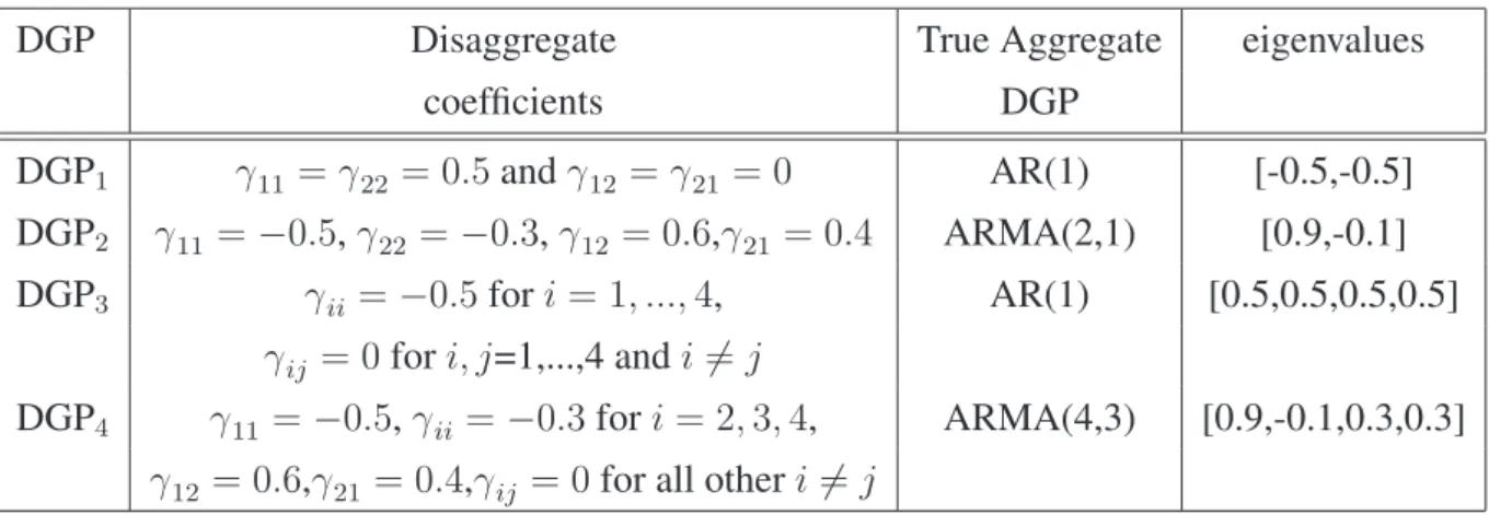
For DGP₁, the parameters in (12) are γ₁₁ = γ₂₂ = 0.5, γ₃₃ = γ₄₄ = 0and γij = 0for i, j =

1, ...,4withi=j, so(1 + 0.5L)y_ta = 2 +νtwithσ2ν = 2for the aggregate process. The eigenvalues of the dynamics in DGP₁ are equal, and the disaggregates y₁, y₂ and the aggregateya all follow an AR(1) process, so slope mis-specification will have a small effect on the relative forecast accuracy. This is the first DGP used in L¨utkepohl (1984).

In DGP₁, the direct forecast of the aggregate and aggregating the disaggregate forecasts yield the same MSFE, since the components of the disaggregate multivariate process are independent and have identical stochastic structure. When the true model is used for estimation, the MSFE differences result only from estimation uncertainty, and not from model mis-specification. Therefore, we can isolate the effect of the estimation uncertainty. The 4-dimensional DGP₃ is constructed in a similar way. DGP₂ differs from DGP₁due to the mutual dependence of the disaggregates. Finally, we construct DGP₄ to approximate our empirical example of US aggregate inflation: Two components are interdependent, whereas the two others behave quite differently.

Table 1:Structure of DGPs for MC simulations: Summary Table

DGP Disaggregate True Aggregate eigenvalues

coefficients DGP DGP₁ γ₁₁=γ₂₂= 0.5andγ₁₂ =γ₂₁ = 0 AR(1) [-0.5,-0.5] DGP₂ γ₁₁=−0.5,γ₂₂ =−0.3,γ₁₂= 0.6,γ₂₁= 0.4 ARMA(2,1) [0.9,-0.1] DGP₃ γ_ii =−0.5fori= 1, ...,4, AR(1) [0.5,0.5,0.5,0.5] γij = 0fori, j=1,...,4 andi=j DGP₄ γ₁₁=−0.5,γii=−0.3fori= 2,3,4, ARMA(4,3) [0.9,-0.1,0.3,0.3]

γ₁₂= 0.6,γ₂₁= 0.4,γij = 0for all otheri=j

DGP1, DGP2, and DGP3, DGP4are 2- and 4-dimensional respectively; population variances areσv_i,t= 1i=1,...,4

The simulations were carried out based onN=1000 repetitions. Additional simulations for other DGPs and different sample sizes did not change the qualitative conclusions. In the paper, we only consider results forT = 100 for all DGPs. All four DGPs are stationary in-sample. In DGP₁ and DGP₃, the aggregate process is an AR(p) model, in contrast to DGP₂ and DGP₄ where the DGPs of the aggregate are an ARMA(2,1) and ARMA(4,3) respectively. Consequently, in DGP₁ and DGP₃, the direct autoregressive (AR) forecast has higher accuracy relative to the other methods, in contrast to DGP₂ and DGP₄where the AR(p) model is mis-specified. DGP₁and DGP₃have a factor structure, where the factor isyawith equal weights for the disaggregates.

As in L¨utkepohl (1984), we generate forecasts from independent samples. Possible extensions are to estimate the models recursively, or from a rolling sample. Results based on recursively expanding samples for DGP₁ and DGP₂ for an initial estimation sample ofR = 100 (R = 200) and out-of-sample period of length P = 40 (P = 100) did not change the ranking of the different methods to forecast the aggregate and resulted in similar root MSFEs (RMSFEs) to independent samples (all additional results available on request).

Forecast methodsWe compare five different methods to forecast the aggregate. 1. Direct forecast only using past aggregate information based on an AR model;

2. forecasting disaggregates with an AR model and aggregating those forecasts (indirect AR);

3. forecasting disaggregates with a VAR including all subcomponents, but no aggregate information, then aggregating those forecasts (indirectVARsub);

4. forecasting disaggregates with a VAR including the aggregate and all subcomponents (except one to avoid collinearity when weights are constant) (directVARagg,sub);

5. forecasting with a VAR including selected subcomponentsyiand the aggregate (directVARagg,yi). All models are estimated by (multivariate) least squares, providing identical estimators to maximum

likelihood under a normality assumption. All simulations assume constant aggregation weights, and are carried out using AIC for selecting the order of the model, since a model selection criterion would be employed in practice when the DGP is unknown.

Simulation with a non-constant DGPTo check analytical conclusions 1,2 and 4 in Section 2.3 in small samples, we implemented a change in the mean and in the innovation variance as well as allowing for non-zero cross-correlations in the innovations in DGP₁ and DGP₂. The change in mean is implemented by changing the intercepts of both subcomponents over the out-of-sample period (a) in the same direction for both components, and (b) in opposite directions. The change in variance is implemented by a change in the variance of the innovation errors over the out-of-sample period. We also carry out simulations for DGPs with different innovation variance or with different cross-correlations of the errors for the entire sample period, including both in-sample and out-of-sample. In the latter experiments we allow for positive as well as negative correlations. Throughout, we investi-gate the impacts of the changes on the relative rankings of the different methods. For comparability, we considerT = 100, independent samples, and AIC is used for lag-order selection.

3.2

Simulation results

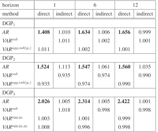
Constant parameter DGP The results are presented in Table 2 and Table 3 in terms of RMSFE relative to the direct AR benchmark model. Only for the direct AR benchmark actual RMSFEs are presented. Table 2 shows that for DGP₁, the direct forecast of the aggregate based only on aggregate information is best for a 1-step ahead horizon, while the indirect forecast of the aggregate using AR models for the component forecasts is ranked second. The VAR based forecast is worst for this particular DGP. The direct and indirect VAR models provide the same RMSFE because including one disaggregate component in the aggregate model when the DGP is 2-dimensional is just a linear transformation of aggregating the disaggregate forecasts (see Section 2.4). The simulation results for DGP₁ are comparable to L¨utkepohl (1987, Table 5.2).

Investigating the RMSFE for all horizons between h = 1 and 12 showed that the differences for horizons larger than 3 were minor, in line with the results in L¨utkepohl (1984, 1987), who only presents results for h = 1andh = 5. At forecast horizonh = 12, all forecasts are almost identical. At larger T (200 and 400, not presented), the RMSFEs of the direct and indirect forecasts of the aggregate are closer: the DGP implies equal population MSEs, so a largerT leads to a decline in both estimation uncertainty and lag-order selection mistakes, and therefore higher forecast accuracy.

Table 2, second panel, shows that for DGP₂, in contrast to DGP₁, the VAR forecasts are most accurate and the direct AR forecast is second best. Even though that DGP is stationary, the two

eigenvalues are substantially different. For DGP₂, including disaggregate information in the aggregate VAR model or forecasting the disaggregates from a VAR and aggregating their forecasts improves forecast accuracy over the other methods.

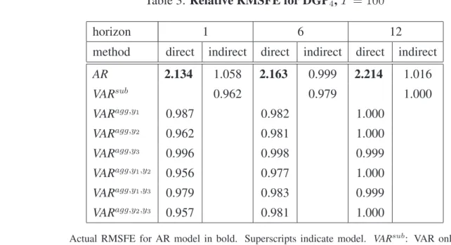
The simulation results for the 4-dimensional DGP₃, with independent components that have the same stochastic structure (as in DGP₁), show that the direct AR forecast is again most accurate (as for DGP₁), but including just one disaggregate is second best forh= 1(see Table 2, third panel). For DGP₄, instead, where the disaggregates are interdependent and follow different stochastic processes, Table 3 shows that including disaggregates in the aggregate model improves over the direct AR fore-cast. The indirectVARsubprovides more accurate forecasts than the direct or indirect AR forecast for

h= 1.

Table 2: Relative RMSFE for DGP₁, DGP₂ and DGP₃,T = 100

horizon 1 6 12

method direct indirect direct indirect direct indirect DGP₁ AR 1.408 1.010 1.634 1.006 1.656 0.999 VARsub 1.011 1.002 1.001 VARagg,sub(y1) _{1.011 1.002 1.001} DGP₂ AR 1.524 1.113 1.547 1.061 1.560 1.035 VARsub 0.935 0.974 0.990 VARagg,sub(y1) _{0.935 0.974 0.990} DGP₃ AR 2.026 1.005 2.314 1.005 2.422 1.001 VARsub 1.018 0.998 0.998 VARagg,y3 _{1.003 1.001 0.999} VARagg,y2,y3 _{1.008 0.996 0.998}

Actual RMSFE for AR model in bold. Superscripts indicate model. VARsub: VAR only including subcomponents;VARagg,sub(yi)_{: VAR with aggregate and subcomponent}y_{i. Lag}

order selection for all models by Akaike criterion.N= 1000. See Table 1 for the DGPs.

Non-constant parameter DGPThe simulations investigating the effects of a change in the mean and in the variance of the disaggregates on the relative forecast accuracy ranking of the different methods, yielded the following results for a 1-step forecast horizon. First, a change in mean does not

Table 3:Relative RMSFE for DGP₄,T = 100

horizon 1 6 12

method direct indirect direct indirect direct indirect AR 2.134 1.058 2.163 0.999 2.214 1.016 VARsub 0.962 0.979 1.000 VARagg,y1 _{0.987 0.982 1.000} VARagg,y2 _{0.962 0.981 1.000} VARagg,y3 _{0.996 0.998 0.999} VARagg,y1,y2 _{0.956 0.977 1.000} VARagg,y1,y3 _{0.979 0.983 0.999} VARagg,y2,y3 _{0.957 0.981 1.000}

Actual RMSFE for AR model in bold. Superscripts indicate model. VARsub: VAR only including subcomponents;VARagg,sub(yi)_{: VAR with aggregate and subcomponent}y_{i. Lag}

order selection for all models by Akaike criterion.N = 1000. See Table 1 for the DGP.

change the ranking of the different methods, whether the intercepts in the disaggregate components change in the same or in the opposite direction. This confirms our analytical results in conclusion 1 in Section 2.3. Second, a change in the error variance of the disaggregate components out-of-sample for DGP₁ still leads to the same ranking of the different methods, with the AR direct having highest forecast accuracy. For DGP₂we get an unchanged ranking of the different methods. Third, changing the variances over the entire sample period, in-sample and out-of-sample, again does not alter rankings for DGP₂, while for DGP₁, all the RMSFEs are very close. Fourth, allowing for cross-correlations between innovation errors (instead of zero cross-correlations) alters the forecast accuracy ranking for DGP₁, but not for DGP₂. Our analytical results show that the error covariance structureper sedoes not affect the rankings of the different methods directly, but it does affect it indirectly through estimation uncertainty, as pointed out in conclusion 7 in Section 2.3. Our simulation results confirm that in small samples the error covariance structure can affect the relative estimation uncertainty substantively.

Summary Overall, including disaggregate variables in the aggregate model helps forecast the aggregate if the disaggregates follow different stochastic structures and are interdependent. The dif-ferences in forecast accuracy are less pronounced for higher horizons, since all the forecasts converge to the unconditional mean. In particular, we find that selecting disaggregates helps to improve forecast accuracy by reducing estimation uncertainty if the number of disaggregates is relatively large.

4

Forecasting aggregate US inflation

In this section, we analyze empirically the relative forecast accuracy of the three methods to forecast the aggregate, investigated analytically and via Monte Carlo simulations in the previous sections, for forecasting aggregate US CPI inflation.

Relation to other empirical studies of contemporaneous aggregation and forecasting The intro-duction discusses the large empirical literature on contemporaneous aggregation and forecasting, and the mixture of outcomes reported as to whether aggregation of component forecasts or forecasting the aggregate from past aggregate information alone provides the most accurate forecasts for aggregate inflation. For euro area countries, or the euro area as a whole, the results depend on the country analyzed, whether aggregation is considered across countries or disaggregate components, the fore-casting methods or model selection procedures employed, the particular sample periods examined (e.g. before and after EMU), and the forecast horizons considered (see, e.g., Hubrich (2005), Benalal et al. (2004), Bruneau et al. (2007), and Marcellino et al. (2003)).

For real US GNP growth, Fair & Shiller (1990) find that disaggregate information helps forecast the aggregate, and Zellner & Tobias (2000), find for forecasting median GDP annual growth rates of eighteen industrialized countries, that forecasts of the aggregate can be improved by aggregating disaggregate forecasts, provided an aggregate variable is included in the disaggregate model and all coefficients are restricted to be the same across countries.

We now consider empirically two very different sample periods for US inflation (see e.g. Atkeson & Ohanian (2001) and Stock & Watson (2007) for recent contributions to predictability changes in US inflation). We investigate whether changes in aggregate US inflation and its components over those different sample periods affects whether disaggregate information helps forecast the aggregate.

4.1

Data

The data employed in this study include the all items US consumer price index (CPI) as well as its breakdown into four subcomponents: food (pf), commodities less food and energy commodities (pc), energy (pe) and services less energy services prices (ps) (Source: CPI-U for all Urban Consumers, Bureau of Labor Statistics). We employ monthly, seasonally-adjusted data, except for CPI energy which does not exhibit a seasonal pattern. Seasonal adjustment by the BLS is based on X-12-ARIMA. We do not consider a real-time data set, since revisions to the CPI index are extremely small. We consider a sample period for inflation from 1960(1) to 2004(12), where earlier data from 1959(1) onwards are used for the transformation of the price level. As observed by other authors (e.g., Stock

& Watson (2007)), there has been a substantial change in the mean and the volatility of aggregate inflation between the two samples. We document that the disaggregate components also exhibit a substantial change in mean and volatility. Aggregate as well as components of inflation, all exhibit high and volatile behavior until the beginning or mid 80s and lower, more stable rates thereafter (see Table 4 for details).

In sections 4.2 and 4.3, we present results of an out-of-sample experiment for two different fore-cast evaluation periods: 1970(1)–1983(12) and 1984(1)–2004(12). The date 1984 for splitting the sample coincides with estimates of the beginning of the great moderation, and is in line with what is chosen in Stock & Watson (2007) and Atkeson & Ohanian (2001). We use the same split sample for comparability of our results to those studies in terms of aggregate inflation forecasts.

Table 4: US, Descriptive Statistics, year-on-year CPI Inflation 1960–1983 all items energy commodities food services Mean 4.86 5.91 3.80 4.75 5.81 Std Deviation 3.41 8.17 2.89 4.11 3.40 1984–2004 all items energy commodities food services Mean 2.99 2.28 1.43 2.93 3.91 Std Deviation 1.06 8.26 1.65 1.26 0.99

Due to the mixed results of ADF unit-root tests for different CPI components and samples, we carry out the forecast accuracy comparisons for the level and the change in inflation. We present the results for the level of inflation, as results for the changes in inflation do not differ qualitatively from those for the level in terms of relative forecast accuracy of the different methods. We evaluate the 1- and 12-month ahead forecasts on the basis of the same forecast origin. The main criterion for the comparison of the forecasts here, as in a large part of the literature on forecasting, is RMSFE.

4.2

Combining disaggregate forecasts or disaggregate variables: AR and VAR

models

Forecasting methods We employed various forecasting methods, with different model selection procedures for both direct and indirect forecasts (forecasting inflation directly versus aggregating subcomponent forecasts). Tables 5 and 6 present the comparisons of forecast accuracy measured in terms of RMSFE of year-on-year (headline) US inflation for forecasting aggregate (all items) inflation using different approaches to forecast an aggregate.

The forecasting models include: (1) a simple autoregressive (AR) model; (2) the random walk (RW) implemented as inflation inT +h being the simple average of the month-on-month inflation rate fromT−12toT, as used in Stock & Watson (2007) referring to Atkeson & Ohanian (2001); (3) a subcomponentVARsubto indirectly forecast the aggregate by aggregating subcomponent forecasts; (4) VARs including the aggregate and all disaggregate components (perfect collinearity between aggre-gate and components does not occur due to annually changing weights in price indices), or a selected number of disaggregate components,VARagg,subandVARagg,subi_{; and (5) an MA(1) (as used in Stock}

& Watson (2007)). Results for factor models are presented in the next section. Model selection pro-cedures selecting the lag length in the various models employed above include the Schwarz (SIC) and the Akaike (AIC) criterion, respectively, with maximum lag order of 13. We find that the AIC-based models generally perform better for US inflation and therefore present results for those models.

The benchmark model for the comparison is the (direct) forecast of aggregate inflation from the AR model, simply forecasting aggregate inflation from its own past (first entry in column labeled ‘direct’ in Tables 5 and 6). This is compared to the indirect forecast from the AR model, i.e. the ag-gregated AR forecasts of the sub-indices, as well as to the other methods of forecasting the aggregate directly (column labeled ‘direct’) or indirectly (column labeled ‘indirect’) using VARs (see above).

The combination of the disaggregate forecasts for all models is implemented by replicating the aggregation procedure employed by the BLS for the CPI disaggregate data. The data are aggregated in levels, taking into account the respective base year of the weights. Historical aggregation weights were provided to the authors by the BLS. For the aggregation of the forecasts, the current aggregation weights are used, since future weights would not be known to the forecaster in real time.

Δ12pagg andΔ12paggsub indicate that the forecast is evaluated on the basis of year-on-year inflation. The models are, however, specified in terms of month-on-month inflation. It should be noted that the ranking of the different forecast methods is not invariant to the selected transformations (see e.g. Clements & Hendry, 1998, pp 68). We found that models formulated in terms of year-on-year inflation provided the same ranking and less accurate forecasts than those for monthly changes in inflation evaluated at year-on-year inflation. Iterative multi-step ahead forecasts are based on the following model (only including one lag of inflation and no other macroeconomic variables as predictors for expositional purposes):πT₊h =αhi₌₀−1β

i

+βhπT, where inflationπtis specified in first differences as (Pt −Pt₋₁)/Pt₋₁. Results for the change in inflation were not qualitatively different from the results for the level of inflation. In the tables values below unity for the relative RMSFE indicate an improvement in that forecast over the direct AR forecast.

Table 5: Relative RMSFE, US year-on-year inflation (percentage points), 1970-1983

horizon 1 6 12

method direct indirect direct indirect direct indirect

Δ12pagg Δ12paggsub Δ12pagg Δ12paggsub Δ12pagg Δ12paggsub AR 0.294 1.337 1.358 1.083 2.985 1.324 RW 1.031 1.378 1.053 1.048 1.045 1.061 MA₍₁₎ 1.395 1.198 1.899 1.828 1.695 1.318 VARsub 1.450 1.241 1.429 VARagg,sub 1.071 1.468 1.129 1.225 1.254 1.437 VARagg,f 1.046 0.992 0.936 VARagg,c 1.017 0.991 0.974 VARagg,s 1.027 0.962 0.939 VARagg,e 1.028 1.065 1.180

Actual RMSFE (non annualized) for AR model in percentage points, for other models RMSFE relative to AR; recursive estimation samples 1960(1) to 1970(1),...,1983(12); lag order selection for all models (except MA(1) model with one lag) by Akaike criterion, max-imum number of lags: p = 13; superscripts indicate model,VARsub: VAR only including subcomponents;VARagg,sub: VAR with aggregate and subcomponents; ‘direct’: direct fore-cast of the aggregate, ‘indirect’: aggregated subcomponent forefore-cast

Table 6: Relative RMSFE, US year-on-year inflation (percentage points), 1984-2004

horizon 1 6 12

method direct indirect direct indirect direct indirect

Δ12pagg Δ12psubagg Δ12pagg Δ12p agg sub Δ12pagg Δ12p agg sub AR₍AIC₎ 0.190 1.528 0.685 1.024 1.261 1.021 RW 1.000 1.617 0.994 1.095 0.955 0.997 MA₍₁₎ 1.037 1.508 1.129 1.134 1.116 1.021 VARsub_(AIC) 1.627 1.155 1.102

VARagg,sub_(AIC) 1.044 1.610 1.107 1.179 1.074 1.111

VARagg,f_(AIC) 0.995 0.903 0.871

VARagg,c_(AIC) 1.053 1.091 1.078

VARagg,s_(AIC) 1.037 1.120 1.177

Results The RMSFE results indicate, first, that the direct forecast is generally more accurate than the indirect forecast of the aggregate, irrespective of whether disaggregate information is included in the aggregate model or not. Second, for the high inflation sample in the 1970s, including one disaggregate in the aggregate model might improve over the direct AR model forecast for longer horizons as well as over the MA(1) (The MA(1) is less accurate than the AR(p)in the first sample period and similar to it in the second (see Stock & Watson (2007), who analyze four different price measures, for similar results for quarterly CPI inflation). Including disaggregate variables in most cases also dominates combining disaggregate forecasts in RMSFE terms. For the latter sample 1984-2004, including food inflation in the aggregate model improves forecast accuracy over the direct AR model for all horizons. Interestingly, including food inflation in the aggregate model also improves over the RW model that performs better in RMSFE terms for the second sample period for a 1-year horizon. It also improves over the MA(1) for all horizons. We apply the Clark & West (2007) test of equal forecast accuracy for the food inflation model against an AR benchmark for a horizon of one month, and find that this RMSFE improvement is significant at the 10% level. It should be noted, however, that the improvement is not significant when using appropriate critical values for testing a set of four models including different disaggregates against the benchmark AR model for the aggregate (see Hubrich & West (2009), also for similar results for other macroeconomic regressors). Overall, the results suggest that variable selection is important in reducing the impact of parameter uncertainty here.

4.3

Disaggregate information in dynamic factor models

We now compare combining disaggregate information by including factors estimated from the dis-aggregate components in the dis-aggregate model with forecasting the dis-aggregate by the benchmark AR model. The analytical investigation showed estimation uncertainty to be an important determinant of the relative forecast accuracy of the different methods to forecast an aggregate. Factor models can reduce estimation uncertainty in comparison with a VAR with many parameters. We employ fac-tor models averaging away idiosyncratic variation in the disaggregate series, and include the facfac-tors, estimated by principal components from disaggregate price information, in the aggregate model.

Under the assumptions in Stock & Watson (2002a, 2002b) the model is identified and the factors and loadings can be estimated. Related studies of approximate factor models have shown consistency of principal components estimators of the factor space, e.g. Bai (2003), Bai & Ng (2002) and Forni, Hallin, Lippi & Reichlin (2000, 2005) . Treatments of classical factor models when the cross-sectional dimensionnis small can be found in e.g. Anderson (1984), Geweke (1977), Sargent & Sims (1977),

Stock & Watson (1991). A larger cross-section relative to T improves asymptotic performance, in that consistency is achieved at a faster rate compared to a small cross-section (see Stock & Watson (1998)). To keep our information set comparable with that in the forecast experiments with VAR models, we retained the same disaggregate variables.

Little is known so far how the size and the composition of the data affect the factor estimates (see e.g. Boivin & Ng (2005)). We are concerned with how factors from disaggregate information affect forecast accuracy of the aggregate economic variable. Since the models considered here are more parsimonious than many VARs considered above, forecast accuracy may be less affected by estimation uncertainty.

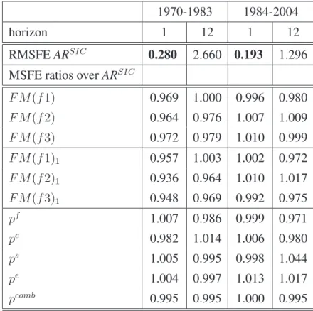
Table 7: US, RMSFE ratios

1970-1983 1984-2004

horizon 1 12 1 12

RMSFEARSIC 0.280 2.660 0.193 1.296 MSFE ratios overARSIC

F M(f1) 0.969 1.000 0.996 0.980 F M(f2) 0.964 0.976 1.007 1.009 F M(f3) 0.972 0.979 1.010 0.999 F M(f1)1 0.957 1.003 1.002 0.972 F M(f2)1 0.936 0.964 1.010 1.017 F M(f3)1 0.948 0.969 0.992 0.975 pf _{1.007 0.986 0.999 0.971} pc _{0.982 1.014 1.006 0.980} ps _{1.005 0.995 0.998 1.044} pe 1.004 0.997 1.013 1.017 pcomb 0.995 0.995 1.000 0.995

RMSFE (not annualized) forAR(SIC)model in percentage points; SIC: lag order selection by Schwarz criterion; Recursive estimation samples 1960(1) to 1970(1),...,1983(12) and 1960(1) to 1984(1),...,2004(12); F M(fi): factor models with i =1,2,3 static factors; F M(fi)₁: factor models with i =1,2,3 factors with 1 lag; principal component estimators of static factors;pf,pc,ps,pe: single predictor models with respective subcomponent as predictor;

pcomb_{: simple average of the forecasts from the four disaggregate component models}

The results from the factor analysis are not directly comparable across all horizons with previous tables except for h = 12, since here direct multi-step ahead forecasts are carried out and forecast

accuracy is evaluated for annualized inflation in line with Stock & Watson (1999, 2007) (instead of year on year inflation as above). We compute the directh-step factor forecasts and single predictor forecasts, and consider forecast combinations of all single predictor models based on the respective disaggregate component with equal weights. The results are presented in Table 7.

For the first sample, disaggregate information helps forecast aggregate US inflation one and twelve months ahead. The improvements over the AR model are up to 6.5% in RMSFE terms (up to 12.5% in MSFE terms). Including one factor is statistically significant for the first sample period for a 1-month horizon by the Clark & West (2007) test of equal forecast accuracy. However, the improvement using factor models is lower in the second sample period. This is in line with what Stock & Watson (2007) find for including real variables in an inflation model.

4.4

Summary of Empirical Results

To summarize our empirical results, overall the direct forecast of the aggregate, either using only past aggregate or using disaggregate information, is more accurate than combining disaggregate fore-casts. Therefore, combining disaggregate information helps over combining disaggregate forefore-casts. Further, including a selected number of disaggregate variables or factors summarizing disaggregate information tends to improve forecast accuracy over forecasting the aggregate directly by only using past aggregate information, in particular in samples with sufficient variability in the aggregate.

5

Conclusions

We presented new analytical results on the relative forecast accuracy of forecasting an aggregate by (1) combining disaggregate forecasts (forecasting the disaggregate variables then aggregating those forecasts), (2) using only lagged aggregate information, and (3) to combine disaggregate information by including a subset of disaggregate components (or a combination thereof) in the aggregate model. In the analytical derivations we investigated the effects of mis-specification and estimation un-certainty on the relative forecast accuracy of the 3 different approaches to forecasting an aggregate, and we extended previous results by allowing for a change in the parameters of the DGP unknown to the forecaster, forecast origin uncertainty and time-varying weights. Decompositions of the sources of forecast errors led us to conclude that relative forecast accuracy is not affected by forecast-origin location shifts and slope changes, whereas absolute accuracy is. This is in contrast to the forecast combination literature, which focuses on combining forecasts of the same variable, where combina-tion helps in the presence of mean shifts in opposite direccombina-tions. Our second main result, in addicombina-tion