DEVELOPMENT OF GPR DATA ANALYSIS ALGORITHMS FOR PREDICTING THIN ASPHALT CONCRETE OVERLAY THICKNESS
AND DENSITY
BY SHAN ZHAO
DISSERTATION
Submitted in partial fulfillment of the requirements for the degree of Doctor of Philosophy in Civil Engineering
in the Graduate College of the
University of Illinois at Urbana-Champaign, 2018
Urbana, Illinois
Doctoral Committee:
Professor Imad L. Al-Qadi, Chair Professor Jeffery R. Roesler Professor John S. Popovics Associate Professor Zhen Leng
ABSTRACT
Thin asphalt concrete (AC) overlay is a commonly used asphalt pavement maintenance strategy. The thickness and density of thin AC overlay are important to achieving proper pavement performance, which can be evaluated using ground-penetrating radar (GPR). The traditional methods for predicting pavement thickness and density relies on the accurate determination of electromagnetic (EM) signal reflection amplitude and time delay. Due to the limitation of GPR antenna bandwidth, the range resolution of the GPR signal is insufficient for thin pavement layer evaluation. To this end, the objective of this study is to develop signal processing techniques to increase the resolution of GPR signals, such that they can be applied to thin AC overlay evaluation.
First, the generic GPR forward 2-D imaging scheme is discussed. Then two linear inversion techniques are proposed, including migration and sparse reconstruction. Both algorithms were validated on GPR signals reflected from buried pipes using finite difference time domain (FDTD) simulation.
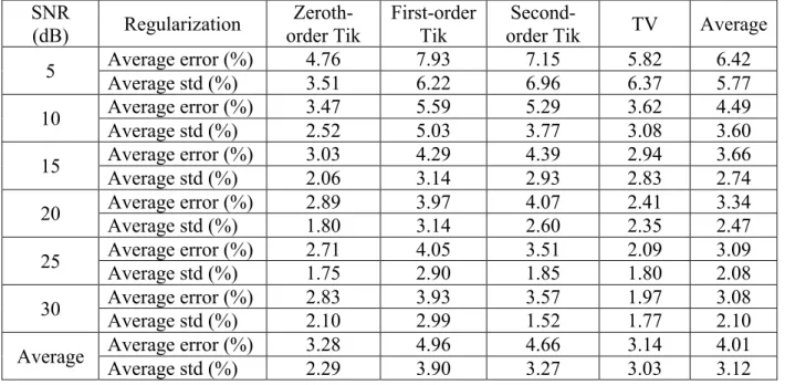
Second, as a special case of the 2-D GPR imaging and linear inversion reconstruction, regularized deconvolution was applied to GPR signals reflected from thin AC overlays. Four types of regularization methods, including Tikhonov regularization and total variation regularization, were compared in terms of accuracy in estimating thin pavement layer thickness. The L-curve method was used to identify the appropriate regularization parameter.
A subspace method—a multiple signal classification (MUSIC) algorithm—was then utilized to increase the resolution of 3-D GPR signals. An extended common midpoint (XCMP) method was used to find the dielectric constant and the thickness of the thin AC overlay at a full-scale test section. The results show that the MUSIC algorithm is an effective approach for
increasing the 3-D GPR signal range resolution when the XCMP method is applied on thin AC overlay.
Furthermore, a non-linear inversion technique is proposed based on gradient descent. The proposed non-linear optimization algorithm was applied on real GPR data reflected from thin AC overlay and the thickness and density prediction results are accurate.
Finally, a “modified reference scan” approach was developed to eliminate the effect of AC pavement surface moisture on GPR signals, such that the density of thin AC overlay can be monitored in real time during compaction.
ACKNOWLEDGEMENTS
I would like to express my earnest gratitude to my advisor Prof. Imad L. Al-Qadi, for his guidance and support during this research. His encouragement and belief in me also helped me overcome the difficulties I encountered in both research and life. I would also like to thank Prof. Jefferey R. Roesler, Prof. John S. Popovics, Prof. Zhen Leng, and Prof. Hasan Ozer for accepting to be in my committee and for taking time to improve my study and dissertation.
My thanks also go to the research engineers at the Illinois Center for Transportation (ICT), Michael Johnson, Shenghua Wu, Greg Renshaw and Jim Meister. I wouldn’t be able to conduct the research without their help. Special thanks also go to my friends and colleagues at the Advanced Transportation Research and Engineering Laboratory (ATREL) for the great time we spent together. I learned a lot from each of them.
Finally, my highest gratitude goes to my mother Wencai Tian and my father Laibin Zhao for their unconditional love and support. They have always been there whenever I need them. Same gratitude also goes to my other family members.
TABLE OF CONTENTS
CHAPTER 1: INTRODUCTION ... 1 CHAPTER 2: BACKGROUND KNOWLEDGE ... 5 CHAPTER 3: GPR IMAGING AND RECONSTRUCTION AND APPLICATION ON
DRAINAGE PIPE EVALUATION ... 14 CHAPTER 4: DEVELOPMENT OF REGULARIZATION METHODS ON SIMULATED GPR SIGNALS TO PREDICT THIN AC OVERLAY THICKNESS ... 39 CHAPTER 5: APPLICATION OF REGULARIZED DECONVOLUTION TECHNIQUES FOR PREDICTING PAVEMENT THIN AC OVERLAY THICKNESSES ... 70 CHAPTER 6: SUPER-RESOLUTION OF 3-D GPR SIGNALS TO ESTIMATE THIN AC OVERLAY THICKNESS USING XCMP METHOD ... 84 CHAPTER 7: PREDICTION OF THIN ASPHALT CONCRETE OVERLAY THICKNESS AND DENSITY USING NONLINEAR OPTIMIZATION ... 100 CHAPTER 8: DEVELOPMENT OF ALGORITHM FOR REAL-TIME THIN AC OVERLAY COMPACTION MONITORING ... 116 CHAPTER 9: FINDINGS, CONCLUSIONS, AND RECOMMENDATIONS ... 142 REFERENCES ... 147
CHAPTER 1: INTRODUCTION
1.1Background
In the United States, there are over 4.2 million miles of paved roads, including more than 76,000 miles of expressways (CIA 2018). To properly manage and maintain this road network, the U.S. spends over $200 million dollars of combined federal, state, and local funding each year (FHWA 2014). Since the completion of the U.S. Interstate Highway system decades ago, the rehabilitation and maintenance of existing pavements have become more important than the construction of new pavements.
The most common pavement maintenance treatment in the U.S. is AC overlay. Layer thickness is an important parameter in pavement design (Huang 2004; Yoder and Witczak 1975; Masad et al. 2012). Newly constructed AC overlay uses thickness for quality control and quality assurance (QC/QA), and existing AC overlay uses thickness to assess pavement condition and predict pavement remaining service life.
Density is another parameter that can greatly influence AC pavement performance. Achieving an appropriate density can reduce the maintenance and rehabilitation cost of the AC pavement, while improper density could result in premature pavement failures (Leng et al. 2012; Lytton et al. 1993). Density can also be used during AC pavement compaction to achieve the desired air voids.
1.2Problem Statement
The traditional way of measuring asphalt pavement thickness and density is by taking core samples and subjecting them to laboratory tests. In addition to being destructive, taking cores can be time consuming and expensive, and can only cover limited locations. An alternative approach
to measuring asphalt density is to use a nuclear density gauge. While this method is nondestructive, the use of radioactive materials requires a special license.
Another alternative is ground penetrating radar (GPR), a special type of radar that can be used to image subsurface targets such as rebar (Soldovieri 2011), drainage pipe (Zhao and Al-Qadi 2017a), archaeological structures (Sala and Linford 2012), landmines (Eide and Hjelmstad 2004), and railway ballast (Al-Qadi et al. 2016). In pavement engineering, GPR has been applied to predict AC pavement thickness Qadi et al. 2003; Al-Qadi and Lahouar 2005) and density (Al-Qadi et al. 2010; Leng 2011). The conventional way of estimating AC layer thickness involves two steps: predicting the dielectric constant of the AC pavement layer using the surface reflection method (Al-Qadi et al. 2001) and calculating the AC layer thickness using the two-way travel time (TWTT) method. The dielectric constant is also used to calculate the density of the AC pavement. Further details will be discussed in chapter 2.
The conventional method for thickness and density estimation relies on the accurate determination of the reflection time and amplitude. Because the bandwidth of the GPR antenna is usually limited, the resulting GPR time domain signal has a limited resolution. For thin asphalt overlay, when the layer thickness is smaller than the signal wave length, the reflection from two adjacent pavement layer interfaces will overlap, making it difficult to accurately determine the reflection time and amplitude. Therefore, signal processing methods need to be developed to solve the problem of thickness and density estimation for thin AC pavement overlay.
1.3Objective
The main objective of this research is to develop signal processing techniques that can increase the range resolution of GPR signals, allowing GPR to be used to predict the thickness and density of thin AC overlay. The research efforts focus on developing linear inversion, non-linear
optimization, and subspace methods. Additionally, this study also aims to develop an algorithm that allows for the real time compaction monitoring of AC pavement using GPR.
To validate the outcome of this study, the proposed algorithms were applied on finite difference time domain (FDTD) simulated data; on GPR data collected from test sections; and on GPR data collected from field tests.
1.4Scope
The dissertation is divided into nine chapters. Chapter 1 briefly introduces the background and the objective of the research. Chapter 2 presents the current state of knowledge including fundamental GPR and EM theories and applications of GPR on pavement engineering. Chapter 3 discusses the generic GPR imaging scheme and reconstruction techniques. In Chapter 4, a linear inversion method, regularized deconvolution is developed and used on FDTD simulated GPR signals. Chapter 5 further validates the regularization technique using field study GPR data. Chapter 6 describes a subspace based super-resolution method, and validates the method on 3-D GPR data using the XCMP method. Chapter 7 presents a nonlinear optimization method that can accurately recover the surface reflection and time delay of GPR signals reflected from thin AC overlay. Chapter 8 describes a “modified reference scan” approach that allows real time compaction monitoring of AC pavement using GPR. Finally, chapter 9 provides the findings and conclusions of the study, and points toward future studies.
1.5Importance of the Study
The accurate prediction of AC overlay thickness and density is important both during pavement construction and service. During the construction of AC overlay, monitoring thickness and density is critical to achieving the proper compaction effort. Thickness and density measurements are also used for QC/QA after pavement construction. Inadequate thickness or
improper compaction will be costly to contractors and the public, as pavements fail. During the service life of pavement, thickness and density information will help experts make smart decisions on rehabilitation time and strategy.
With further development of this study, the GPR system can be integrated with an asphalt compactor roller to achieve real time compaction monitoring of both regular AC pavement as well thin AC overlay. This could potentially help to achieve optimum AC pavement compaction performance.
CHAPTER 2: BACKGROUND KNOWLEDGE
2.1 AC Overlay
Pavement deteriorates over time due to traffic loads and environment effects. Pavement preservation is a proactive approach to maintaining the existing highway, while pavement rehabilitation addresses the repair of part of the pavement when deterioration happens (IDOT 2010). Well-constructed pavements, such as full-depth asphalt pavement, need only functional improvements over time, rather than structural enhancements (Newcomb 2009). As the most common pavement preservation and rehabilitation treatment, asphalt concrete (AC) overlay can be used for either structural or non-structural purposes. Structural overlays are used to increase pavement structural capacity, while non-structural asphalt overlays are frequently used to improve the functionality of a pavement, including the improvement of friction and ride quality, correcting surface cracks, and reducing noise. Non-structural overlays are usually thin overlays with thicknesses ranging from 12.7 mm to 38.1 mm (Newcomb 2009). Thin AC overlays have advantages over other pavement rehabilitation and preservation methods, including low life cycle cost, less dust generation during construction, and the ability to be constructed in stages (Newcomb 2009).
2.2 GPR Principles
2.2.1 EM theories
The classical EM phenomenon is governed by a set of Maxwell’s equations. While Maxwell’s equations in the integral form are valid everywhere, the differential form in terms of free charges and currents is more convenient for analyzing physical problems:
∇𝐸#⃗ =&', (2-1)
∇𝐻##⃗ = 0, (2-2)
∇ × 𝐸#⃗ = −𝜇-.-/##⃗, (2-3)
∇ × 𝐻##⃗ = 𝐽⃗ + 𝜀-3#⃗-/. (2-4)
where 𝐸#⃗ is electric field intensity (Volts/meter), 𝐻##⃗ is magnetic field intensity (Amps/meter), 𝜀 is permittivity of medium (Farads/meter), 𝜇 is permeability of free space (Henrys/meter), 𝐽⃗ is the electric current density (Amperes/meter2), and 𝜌 is the electric charge density (coulombs/meter3).
Faraday’s induction law (2-3) shows that a changing magnetic flux can generate an electric field. The Maxwell-Ampere’s law (2-4) shows that an electric current or a changing electric field can generate a magnetic field. Gauss’ law (2-1) pertains to static electric fields, showing that the electric field lines originate from positive charges and terminate at negative charges. Gauss’ law for magnetism (2-2) shows that magnetic flux lines don’t have origins and must form a circle. In this study, the pavement mediums are assumed to be lossless, non-magnetic, homogeneous, isotropic, and non-dispersive.
In the application of GPR, the target is usually in the far field region of the antenna. In the far field of an antenna, the EM field exhibits local plane wave behavior. If we assume the EM wave is propagating in the z direction, the EM filed is linearly polarized (the most general case being elliptically polarized) with an electric field only in the x direction. Then, by solving Maxwell’s equations, the harmonic plane wave solution in a lossless medium (the conductivity 𝜎 is zero) can be expressed as follows:
𝐸(𝑧) = 𝐸9:cos (𝜔𝑡 − 𝛽𝑧), (2-5)
where 𝐸9: and 𝐻9B are arbitrary constant values, Z = 3DE .DF =
G
' is the wave impedance, 𝜔 is the angular frequency, and 𝛽 = 𝜔√𝜇𝜀 is the phase constant.
The EM wave velocity v can then be calculated as:
ν =𝜔 𝛽 =
1 √𝜇𝜀 .
(2-7)
In free space, the EM wave velocity is equal to L
MGD'D = 3 × 10
O𝑚/𝑠, which is the speed
of light in free space.
If the plane wave is normally incident on an interface of medium 1 and medium 2, the reflection coefficient R and transmission coefficient T are:
R =𝜂U− 𝜂L
𝜂U+ 𝜂L , (2-8)
T = 2𝜂U 𝜂U+ 𝜂L ,
(2-9)
where 𝜂L = M𝜇L/𝜀L and 𝜂U = M𝜇U/𝜀U are the intrinsic impedance of medium 1 and medium 2, respectively. This is Snell’s law of reflection and transmission in the normal incident case. If medium 2 is a perfect conductor such as metal, then , R = -1, and T = 0, meaning that all of the EM waves are flipped and reflected back.
2.2.2 GPR systems
Electrical signals are transmitted via transmission line or through empty space. Antennas are essentially transducers that can convert electrical signals from transmission lines to empty space, or vice versa. According to IEEE, an antenna is defined as “that part of transmitting or receiving system that is designed to radiate or to receive EM waves” (IEEE 1993). GPR, in contrast, is a type of radar whose purpose is to locate targets or interfaces buried with earth material (Daniels
2 0
A GPR system consists of a control unit, antenna, and power supply. The control unit contains the electronics which generate an incident electric signal to the antenna. It is built in with a computer or connected to an outside computer which operates the GPR system and stores the collected GPR data. GPR has three common signal types: pulsed signals, stepped frequency signals, and frequency-modulated signals. A GPR antenna serves as the transmitter and receiver to convert between electrical signals and EM waves. GPR antennas can be either ground-coupled or coupled. Ground-coupled antennas have the advantage of deeper penetration depth, while air-coupled antennas can be mounted on vehicles and can travel at highway speed. Other instruments such as distance measuring instrument (DMI) and GPS can also be used together with GPR to provide the location of the GPR scans.
This study mainly uses an air-coupled GPR system with horn antennas manufactured by Geophysical Survey Systems, Inc. (GSSI). Figure 2-1 shows two 2GHz air-coupled antennas mounted on a van. Figure 2-2 shows SIR20, a GPR control unit. Figure 2-3 shows the DMI and GPS antennas that are used during GPR data collection.
Figure 2-2 SIR20 – GPR control unit
Figure 2-3 GPS antenna (left) and DMI (right)
2.3 GPR Applications in Asphalt Pavement
2.3.1 Layer thickness estimation
The most successful application of GPR on asphalt pavement is the estimation of layer thickness using the surface reflection and two-way travel time (TWTT) method. Figure 2-4 shows a typical GPR signal reflected from a two-layered AC pavement, where “Tx/Rx” represents a monostatic air-coupled antenna. The surface AC layer has a dielectric constant of 𝜀L and thickness of ℎ; the second layer (leveling binder or the old pavement) has a dielectric constant value of 𝜀U. A1 and A2 are the amplitudes of the reflection from the surface and the bottom of the surface layer,
be noted that the reflection coefficient at the first layer and second layer interface is positive in Figure 2-4, assuming 𝜀U < 𝜀L.
Figure 2-4 GPR signal reflected from a two-layered AC pavement
In the scenario shown in Figure 2-4, the surface layer thickness can be determined by:
ℎ = (𝑣∆𝑡)/2, (2-10)
where ∆𝑡 is the TWTT between the reflection from the surface and the reflection from the bottom of the surface, and
𝑣 = 𝑐/M𝜀L (2-11)
is the speed of the EM wave in the surface layer, and 𝑐 = 3 × 10O𝑚/𝑠 is the speed of light in free space. According to equation (2-8), the dielectric constant of the surface layer can be determined using the following equation:
𝜀L = ^1 + 𝐴L⁄𝐴` 1 − 𝐴L⁄𝐴`b
U
, (2-12)
where 𝐴` is the amplitude of the reflection from a copper plate.
A similar procedure can be performed on each layer to find its dielectric constant and thickness.
Al-Qadi et al. (2003) report that the TWTT and surface reflection method shown in equations (2-10) through (2-13) provide an AC layer thickness average estimation error of 2.9%, using GPR data collected from AC pavements 100 mm to 250 mm thick. Another way to estimate AC pavement thickness is to use the common midpoint method (Lahouar et al. 2002), which requires multiple GPR channels.
2.3.2 Density estimation
AC pavement density can be predicted by relating the dielectric constant of the AC layer to its bulk specific gravity (𝐺de). It has been suggested that an exponential regression relationship can be used (Saarenketo 1997). However, that is a simplified approach which was verified only on certain mixture types; it also relies on calibrating the relationship for each AC mixture type.
A more generic model can be developed using EM mixing theory (Shivola 1989). There are three existing EM mixing models: the complex refractive index model (CRI), the Rayleigh mixing model, and the Böttcher mixing model (Sihvola 1989; Böttcher 1978; Behari 2006). Beaucamp et al. (2013) used the Lichtenecker-Rother equation, which is a generalized CRI model, to predict asphalt mixture density from GPR. The study also used a method to correct for the effect of vehicle-mounted antenna vibration on GPR signals, which increases the density prediction accuracy. The study concluded that the proposed methods can be used for asphalt pavement
mixing model, using a shape factor of -0.3. The new model is referred to as the Al-Qadi Lahouar Leng (ALL) model (Al-Qadi et al. 2010; Leng 2011). It was concluded that the ALL model outperforms other EM mixing models (Leng et al. 2011; Leng et al. 2012). The ALL model is presented below: 𝐺de = 𝜀fg − 𝜀e 3𝜀fg − 2.3𝜀e−1 − 2.3𝜀1 − 𝜀e+ 2𝜀e fg 𝜀h − 𝜀e 𝜀h− 2. 3𝜀e+ 2𝜀fg ∙1 − 𝑃𝐺hke−1 − 2. 3𝜀1 − 𝜀e+ 2𝜀e fg ∙ 1𝐺dd , (2-13)
where 𝜀fg is the dielectric constant of the asphalt mixture, 𝜀e is the dielectric constant of the asphalt binder, 𝜀h is the dielectric constant of the aggregate, 𝑃e is the asphalt binder content, 𝐺hk is the effective specific gravity of the aggregate, and 𝐺dd is the maximum specific gravity of the AC mixture. 𝜀e is set as constant 3. 𝐺dd, 𝐺hk and 𝑃e are known from AC mix design. 𝜀h, however, needs to be determined using calibration from core data.
2.4 Super-Resolution of GPR Signals
As explained in section 1.2, the resolution of GPR signals need to be increased for its effective application to thin AC overlays. To this end, signal processing techniques, known as super-resolution techniques, need to be applied. The most common method to recover the layer reflectivity and thickness is deconvolution in either time or frequency domain (Riad 1986), which requires prior knowledge of the incident signal. The details of the deconvolution method will be discussed in chapter 4. If the incident signal is unknown, a blind deconvolution approach based on optimization can instead be used to recover the layer structure (Li 2014; Jia et al. 2017). Recently, machine learning algorithms have also been applied to GPR signal super-resolution. For example, Le Bastard et al. (2014) used a support vector machine (SVM) to find the thickness of thin pavement layer; however, machine learning algorithms usually require large amounts of data for
model training. Another class of super-resolution algorithms are based on subspace analysis, such as MUSIC (multiple signal classification) algorithm (Schmidt 1986; Wax and Kailath 1985; Le Bastard et al. 2007; Zhao and Al-Qadi 2018); these approaches usually require knowledge of the noise subspace. Ihamouten et al. (2018) studied the stepped frequency GPR full wave inversion problem (Lambot et al. 2004) using optimization in the frequency domain to consider the near-field condition and vibration. The dielectric and thickness of pavement structures were predicted with good accuracy.
In this study, both traditional deconvolution methods and optimization methods will be discussed. Additional techniques will be proposed to either stabilize the solution or increase the result accuracy. The details will be covered in following chapters, especially in section 4.2. 2.5 Summary
In this chapter, the thin AC overlay was introduced, and the importance of the thin AC overlay thickness and density estimation was emphasized. An introduction to GPR principles was then provided, including basic EM wave theory and typical GPR system composition. Furthermore, the traditional methods of measuring AC pavement thickness and density were described, including the surface reflection method, the TWTT method, and the ALL model. Finally, the existing super-resolution techniques were briefly reviewed with more details to follow in subsequent chapters.
CHAPTER 3: GPR IMAGING AND RECONSTRUCTION AND
APPLICATION ON DRAINAGE PIPE EVALUATION
3.1 Background and Objective
This chapter presents an overview of the generic GPR imaging and reconstruction technique. The GPR target imaging forward problem is a linear transformation under certain assumptions, and the reconstruction of GPR targets is a classic linear inversion problem. The general 2-D imaging and reconstruction equations will be derived. The problem of 1-D AC pavement imaging is then a special case of the general imaging/reconstruction problem.
In section 3.2, the GPR imaging forward problem will be formulated. In section 3.3, different GPR image reconstruction techniques will be discussed. In section 3.4, the GPR image reconstruction methods discussed in section 3.3 will be applied to a case study: a drainage pipe condition assessment. Section 3.5 summarizes the chapter.
3.2 GPR Imaging
A GPR transmitter antenna sends EM waves toward the ground and the EM waves are reflected from the targets. The GPR receiver antenna then receives the reflected signal. The GPR target can be anything that has an impedance contrast with the surrounding environment, such as metal objects or air voids.
The processing of general synthetic aperture radar data can be found in the literature (Soumekh 1999). As a special type of radar, GPR captures images of three-dimensional targets into a radargram by moving the transmitter/receiver along a straight line. The target is defined by its impedance property. The radargram is a 2-D image, with its vertical dimensional being the reflection time, or fast time, and the horizontal dimension being the trace number. The trace number represents the signal collection time, or the slow time. An example of the GPR imaging is shown in Figure 3-1. In this example, two rebars embedded in concrete were scanned by a
monostatic GPR system with central frequency of 900 MHz, modeled using a FDTD simulation. The obtained radargram shows two hyperbolas, representing the reflection from rebars, as well as a horizontal line, which is the direct coupling pulse. The antenna is assumed to be ground-coupled so there is no ground surface reflection.
Figure 3-1 GPR imaging of rebars embedded in concrete
The general GPR imaging process is described by Maxwell’s equations (Jin 2011). However, under certain assumptions, the imaging scheme can be simplified:
1) The first assumption made in this study is that the target is two-dimensional. This reduces the transverse dimension and greatly reduces the problem complexity.
2) The second assumption is that multiple reflection can be neglected. This assumption is true when the targets are placed far away from each other and there is no target that “shadows” other targets. This also ensures that the target space is sparse.
3) The third assumption is that the targets are thin, in the sense that the dimensions of the targets are small compared with the EM wavelength (i.e., a target dimension of less than a tenth of the EM wavelength).
Under these assumptions, the GPR imaging system is linear (Soldovieri 2011). Another way to explain the linearity is that the radargram is simply the superposition of all radargrams generated by each of the single point targets in the target space.
It is easiest to consider the GPR imaging process in the vector space signal processing content, as shown in Figure 3-2. First, we begin with a 2-D target, such as the one shown in Figure 3-1. We then vectorize the image by stacking the columns of the image to get an input vector 𝑥⃗ ∈ 𝑋, where vector space X is the span of all possible vectors 𝑥⃗. Using the same technique, the 2-D radargram from Figure 3-1 can also be vectorized as a vector 𝑦⃗ ∈ 𝑌. Both input 𝑥⃗ and output 𝑦⃗ are in discrete domains with certain discretization steps that meet the Nyquist sampling criteria (i.e., the sampling frequency is at least twice that of the highest frequency band-limited signal) to prevent aliasing. The linear system serves as the transfer function between the input vector space X and the output vector space Y. Because the system is assumed to be linear, it can be represented by a matrix H, with the input and output having the following simple relationship:
𝑦⃗ = 𝑯𝑥⃗. (3-1)
Figure 3-2 GPR imaging of 2-D target under linearity assumptions
The system matrix H is determined by the excitation source, attenuation factor and impedance of the media, and the dimension of both input and output vector space. Another way to obtain matrix H is through simulation; i.e., using FDTD to simulate the single radargram generated
by each of the pixel in the input space. The latter method is more accurate; however, this can be extremely tedious when the input space is highly dimensional. Therefore, in the following drainage pipe example, we will use the first method to generate system matrix H.
3.3 GPR Image Reconstruction
3.3.1 Migration
Under the GPR imaging scheme described in the section above, the objective was to find the GPR target from the obtained radargram. Considering the aforementioned assumptions, this is a linear inverse problem: find 𝑥⃗r that can approximate 𝑥⃗. In order to do this, a linear inverse operator was established, such that:
𝑥⃗r = 𝑯∗𝑦⃗. (3-2)
Note that here we didn’t follow the mathematical convention: H* is not the complex conjugate of matrix H, but a matrix symbol to represent the inverse operator we need. The easiest solution to this problem is to select the inverse operator to be the adjoint operator:
𝑯∗ = 𝑯𝑻. (3-3)
Migration is a method commonly used in seismic wave reconstruction (Gazdag and Sguazzero 1984). The migration method refers to a series of similar methods—such as Kirchhoff migration (Bleistein and Gray 2001), Hagedoorn migration (Bleistein 1999), pre-stack migration (Berkhout 1986), and f-k migration (Gilmore et al. 2006)—which was demonstrated to be equivalent to the synthetic aperture radar technique shown in Soumekh (1999). Those migration techniques are equivalent to the adjoint operator shown in equation (3-3), which projects each pixel in the radargram space to the target space pixels, which contribute to that pixel in the radargram space.
A practical way to implement the migration technique is to use the synthetic aperture focus technique (SAFT; Gilmore et al. 2006). The procedure is summarized below:
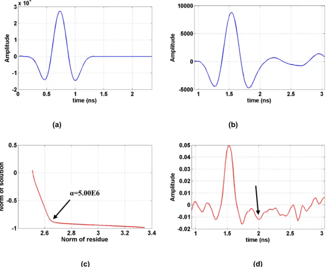
1) Remove the radargram background (direct coupling) to obtain multiple traces (Figure 3-3(a)). 2) For each trace, convert time to distance and generate the reflection “circles” (Figure 3-3(b)).
This step projects the radargram data back to the corresponding target space. 3) Superpose all circles to generate the desired target (Figure 3-3(c)).
4) Perform image thresholding (Figure 3-3(d)).
The migration algorithm has a complexity of O(n).
(a)
Figure 3-3 SAFT technique procedures: (a) Radargram after removal of direct coupling pulse; (b) “circle” generated by one of the trace; (c) superposition of all “circles”; (d) image
(b)
(c)
(d) Figure 3-3 (cont.)
3.3.2 Sparse reconstruction
The intuitive way to find the exact target vector 𝑥⃗ from Equation (3-1) is to find the inverse of matrix H:
𝑯∗ = 𝑯u𝟏. (3-4)
However, system matrix H is not always an invertible square matrix. An alternative way is to find the minimum square error (MSE) solution:
𝑥⃗r = 𝒂𝒓𝒈𝒎𝒊𝒏{‖𝑯𝒙##⃗ − 𝒚##⃗‖𝟐}, (3-5) where ‖∗‖ represents the L-2 norm and “argmin” means to find the argument x which minimizes the inner expression. The resulting inverse operator is given by the pseudo-inverse of system matrix H:
𝑯∗ = (𝑯𝑻𝑯)u𝟏𝑯𝑻. (3-6)
However, the size of matrix H is too large to invert directly. If the input space has a dimension of 20,000—i.e., the target image has 20,000 pixels—and the output space has a dimension of 20,000, matrix A will be a 20,000 x 20,000 matrix. Inverting such a matrix will require a large amount of time since matrix inversion (using Gauss–Jordan elimination) has a complexity of 𝑂(𝑛…). There are algorithms that can solve the pseudo-inverse more efficiently: e.g., general singular value decomposition (GSVD). The detailed derivation can be found in Aster et al. (2013). In addition, matrix H is ill-posed. A small perturbation in the output 𝑦⃗ (e.g. noise) will result in huge fluctuation in the reconstructed target 𝑥⃗r and, therefore, regularization is needed. There are several regularization methods available. A common method is the Tikhonov regularization:
𝑥
where is the regularization parameter, is a matrix with full rank. The matrix L can be chosen as an identity matrix, first-derivative matrix, and second-derivative matrix, etc.; the corresponding regularizations are called the zeroth-, first-, and second-order Tikhonov regularization, respectively.
Sparse reconstruction regularization was used in this study because the GPR target space is sparse by nature (see second assumption in Section 1). Since the L-0 norm calculates the number of non-zero elements in a vector, the following L-0 norm regularization guarantees that the solution has a minimum number of non-zero elements:
𝑥⃗r = 𝒂𝒓𝒈𝒎𝒊𝒏{‖𝑯𝒙##⃗ − 𝒚##⃗‖𝟐+ 𝜶‖𝒙##⃗‖
𝟎}. (3-8)
It was found that when the input vector is sparse (which is the case in this study), the total variation will also give the sparse solution (Ramirez et al 2013):
𝑥⃗r = 𝒂𝒓𝒈𝒎𝒊𝒏{‖𝑯𝒙##⃗ − 𝒚##⃗‖𝟐+ 𝜶‖𝒙##⃗‖
𝟏}. (3-9)
In this study, total variation regularization was used because it is easier to implement due to the convexity of the problem.
There are many ways to solve the total variation problem, including the iteratively reweighted least squares (IRLS) method (Aster et al. 2013). In this study, the spectrum projected gradient method (SPG) was used due to its efficiency (Van Den Berg and Friedlander 2008). Equation (3-9) can be rephrased as the LASSO (least absolute shrinkage and selection operator) problem (Van Den Berg and Friedlander 2008):
𝑥⃗r = 𝒂𝒓𝒈𝒎𝒊𝒏{‖𝑯𝒙##⃗ − 𝒚##⃗‖𝟐, 𝒔𝒖𝒃𝒋𝒆𝒄𝒕𝒆𝒅 𝒕𝒐 ‖𝒙##⃗‖
𝟏 ≤ 𝝉}, (3-10)
where is a parameter associated with the regularization parameter in equation (3-9). The procedure of the SPG algorithm is then summarized in the following:
U
a L
2) Gradient descent: 𝑥⃗•–L = 𝑥⃗•− 𝛼𝛻:, where 𝛼 is the step length.
3) Project 𝑥⃗•–L to the one-norm ball of radius 𝜏 to update 𝑥⃗•–L. The detailed procedure of this one-norm projection is explained in (Van Den Berg and Friedlander 2008).
4) Iterate the procedure until small enough error is achieved. The SPG algorithm has a worst-case complexity of 𝑂(𝑛 log 𝑛).
3.4 Application of GPR Image Reconstruction on Drainage Pipe Evaluation
3.4.1 Introduction to drainage pipe condition assessment
Drainage design is important for the operation of traffic on highway or airport pavement. Malfunction of the drainage pipes can cause saturation of the pavement, resulting in serious flooding issues, a decrease in strength or stability, and pavement deficiencies including pumping, swelling, frost damage, and aggregate stripping. These issues jeopardize a pavement’s structural ability to support heavy axle loads and decreases its functionality. A typical pavement drainage system consists of a permeable drainage layer to drain water beneath the pavement, a collector system to drain water out of pavement, an outlet, and a filter layer to prevent fine particles from entering the permeable layer (CDOT, 2015). Drainage pipes are a common collector system. The quality of drainage pipes can be impaired due to poor installation and lack of maintenance. Therefore, it is necessary to monitor the condition of the drainage system to ensure that they are well positioned and not clogged (by soil or foliage).
Once the drainage pipes are built, it is difficult to track their condition without excavation as they are buried deep under the pavement. There are, however, several non-destructive ways to inspect drainage pipes. The most common approach is to use a pipe crawler, or a pipe crawling inspection robot (Roman et al. 1993). The pipe crawler is a computer with multiple sensors, including a closed circuit television (CCTV) system and a fisheye camera. The pipe crawler is
remotely controlled from the ground and moves inside the pipe collecting drainage pipe information, including cracking, clogging, and corrosion.
Using pipe crawlers greatly reduces the danger involved in human inspection. A fully autonomous pipe crawler system called “KANTARO” was developed in Japan and operates without the need for any human navigation (Nassiraei et al. 2006). However, the inspection speed of the pipe crawler is not fast enough to survey large distances of pipes. Another sensing method is the laser-based scanning system, which uses structured light as its source. The laser-based scanning system can provide a more accurate measurement of the shapes and defects of the pipes (Sinha 2003). Other NDT techniques have also been used to monitor drainage pipe conditions, including ultrasonic inspection, eddy current testing, infrared sensing, and acoustic emission mentoring (Sinha 2004). However, those methods provide less accurate results when the pavement structure is not so uniform. An overview of different NDT methods to assess drainage pipe condition can be found in Duran (2002).
All NDT techniques mentioned above require access to the drainage pipes, usually provided by sending a robot. This is sometimes impossible, as in the case where manholes are not accessible or the drainage pipes are filled with water or soil. An alternative NDT method is GPR.
GPR has already been used in drainage pipe detection. Allred et al. (2004a) used four methods (geomagnetic surveying, EM induction, resistivity, and GPR) to detect buried drainage pipes and concluded that only GPR provided good performance. Another study conducted by the same group using different central frequencies showed that GPR can be used to detect drainage pipes effectively under different moisture and temperature conditions (Allred et al. 2004b). Zeng and McMechan (Zeng and McMechan 1997) used ray-based GPR simulation data on drainage pipes and found that different GPR data characteristics can help identify the material, size, content,
fluid levels, and shapes changes of the drainage pipe. The study was based on characterization of the hyperbolic shaped GPR signal done by humans. Youn and Chen (2004) successfully automated this process by developing a two-step neural network algorithm to transform the obtained hyperbola to actual drainage pipe image. With this technique, the accuracy of detecting drainage pipes increases, because operator experience is no longer needed for the identification of drainage pipes. The drawback of this method, as with any machine learning algorithm, is that it requires a large amount of GPR data and associated ground truth to train the neural network model.
Image reconstruction is an alternative way to recover the original drainage pipe target. In this section, both migration reconstruction and sparse reconstruction will be applied on FDTD simulated GPR signals to reconstruct drainage pipes with different sizes, locations, and conditions. The results of both methods are compared in terms of accuracy and computation speed.
3.4.2 FDTD modeling
Computational electromagnetics, which can solve Maxwell’s equations numerically, is an important tool for modeling EM phenomenon in radio frequency. There are generally two methods of calculating computational electromagnetics: the time-domain method and the frequency domain method. Frequency methods are good for dispersive media applications, while time-domain methods are good for broadband problems with only a few excitations (Jin 2011). Due to the characteristics of GPR pulses, a time-domain method, FDTD method, and an open source program, GPRMax (Warren et al. 2016), were used in this study to model GPR signals reflected from two drainage pipes embedded in concrete pavement.
Cases with more drainage pipes are not considered in this study because of the large computational cost of the sparse reconstruction algorithm. The two drainage pipes in this study were 0.2 m apart and had different depths, sizes, and contents. The seven models are summarized
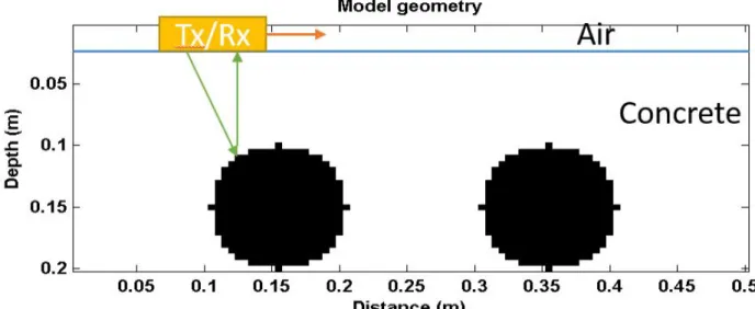
in Table 3.1. The diameters of the two drainage pipes ranged between 6 cm and 10 cm, with a depth ranging between 0.11 m and 0.15 m. In practice, pavement drainage pipes are usually buried deeper. For this study, a shallower depth was selected because a deeper drainage pipe would generate a larger model (in terms of number of pixels in the target space) and would increase the computational time of the reconstruction algorithms, especially for the sparse reconstruction algorithm. The drainage pipes were assumed to be occupied by air, water, or soil, with relative permeabilities (or dielectric constants) of 1, 82.4, and 30, respectively. Since the pipe wall (clay or concrete) is usually thin compared with the EM wavelength, wall thickness was neglected. The study focused on estimating the diameter and the depth of the drainage pipes, and determining whether the drainage pipes were empty or occupied by water or soil.
Table 3-1 FDTD Models of Drainage Pipes Model No. Diameter (m) Depth (m) Content
1 0.1 0.13 Air 2 0.1 0.13 Water 3 0.1 0.13 Soil 4 0.08 0.13 Air 5 0.06 0.13 Air 6 0.06 0.11 Air 7 0.06 0.15 Air
An example configuration of the drainage pipes (Model 1) is shown in Figure 3-4. Concrete was assumed to be homogeneous, its dielectric constant was assumed to be 7, and its conductivity assumed to be 0.01 S/m. The GPR transmitter and receiver were placed 5 cm apart near the concrete surface. The GPR system is ground-coupled, so there is no surface reflection in the obtained radargram. The GPR antenna is broadband with central frequency of 900 MHz. The excitation source is Ricker wavelet. The spatial step of the FDTD model was set to 5 mm in both the x and y direction. The time step dt was set to 1.179*10-11 sec, which was determined using the
d𝑡 ≤ L
œ•(ŸE) ž –(ŸF) ž , (3-11)
where d𝑥 and d𝑦 are the spatial discretization steps in horizontal and vertical directions, respectively, and d𝑡 is the time step.
The radargram obtained from the FDTD simulation is shown in Figure 3-5.
Figure 3-5 Radargram from FDTD simulation.
3.4.3 Results
Using both migration and the sparse reconstruction technique, the results of the reconstructed targets are presented in this section. The drainage pipe contents were obtained from the reconstructed images; the depths and diameters of the drainage pipes were estimated and compared with the true model. The computational time of both methods was also compared.
Figures 3-6 and 3-7 show the reconstructed targets from Models 1 and 2 using both the migration and the sparse reconstruction technique. First, we observed that both migration and the sparse construction methods could only reconstruct the top part of the drainage pipes. This is because of the violation of the second and the third assumption: the drainage pipes are thick, and the EM waves cannot penetrate the structure to reach the bottom part of the pipes. Second, we noted that when the drainage pipes are empty (i.e., occupied by air), the reconstructed image has
positive pixel values; however, when the drainage pipes are occupied by soil or water, the target has negative pixel values. This makes sense if we consider the dielectric constant contrast of the target and the ambient concrete and the EM wave reflection law. We can then estimate the content of the drainage pipes: if the target has positive pixel values, the pipe is empty (Figure 3-6); if the target has large negative pixel values, then the pipe is occupied by water (Figure 3-7); if the target has small negative pixel values, the pipe is occupied by soil (Figure 3-8). The content estimation result is shown in Table 3-2.
The reconstruction performance of the two methods was also studied. The reconstructed images from both methods have artificial noise in the target because of violating the linearity assumption of the model. Specifically, the “inner pipe” shown in the sparse reconstruction could be due to multiple reflection inside the pipe or between adjacent pipes. The sparse reconstruction is nonetheless more accurate than the migration method. This is due to the fact that adjoint operator cannot give an exact reconstruction of the input vector.
In addition, the migration method always requires selecting the proper threshold and is, therefore, not a deterministic algorithm, while the sparse reconstruction is an automatic algorithm.
Figure 3-6 Reconstructed image of Model 1: (a) Migration reconstruction, and (b) sparse reconstruction
Figure 3-7 Reconstructed image of Model 2: (a) Migration reconstruction, and (b) sparse reconstruction.
Figure 3-8 Reconstructed image of Model 3: (a) Migration reconstruction, and (b) sparse reconstruction.
The reconstruction of Models 3 to 6 show similar results as with Models 1 to 3, and is therefore not presented in this dissertation. From the two examples above, we noticed that we can easily find the pipe depth and diameter from the sparse reconstructed result; however, for the migration reconstructed results, a quantitative determination of the pipes parameters is made difficult because of the inaccurate reconstruction. Table 3-2 shows the depth and diameter estimation of the sparse reconstruction methods. The estimation process is illustrated in Figure 3-9. The radius of the pipe is estimated by first finding the center of the circle (which is an equal
distance from all points on the circle in a MSE sense), then finding the distance from center of the circle to the top on the circle (we can also average all radii to get a more accurate estimation). The depth of the drainage pipe is the distance between the pipe center and the antenna position. The cover depth of the pipe can be then calculated by subtracting the pipe radius from the depth of the pipe.
Figure 3-9 Estimation of drainage pipe size and location.
Table 3-2 Depth, Diameter and Content Estimation of the Reconstructed Pipes Using Sparse Reconstruction and Computation Speed of Both Methods
Model No. Diameter (m) Depth (m) Content
Computation Time (s) Migration Sparse Reconstruction
1 0.110 0.135 Air 0.0242 2.10 2 0.110 0.135 Water 0.0212 1.30 2 0.110 0.135 Soil 0.0231 1.00 3 0.090 0.135 Air 0.0246 3.30 4 0.07 0.130 Air 0.0309 1.70 5 0.07 0.150 Air 0.0261 2.80 6 0.07 0.110 Air 0.0206 1.10
Table 3-2 shows that the estimated pipe diameters and depths are very close to the ground truth shown in Table 3-1. The absolute error is within 0.01 m. Considering that the model is
discretized by steps of 0.005 m, the error is within two steps. Unlike thin 2-D targets, such as rebars, the MSE of the original target and the reconstructed targets cannot be computed, since we are only reconstructing the top surface of the drainage pipes instead of the full target image.
The last two columns in Table 3-2 show the computation time of both methods using a computer with an Intel i7 processor. The computation time of sparse reconstruction is more than 10 times that of the migration method. This is mainly because of the computational complexity difference of the two reconstruction methods: the migration method has time complexity of O(n), and the sparse reconstruction has worst-case complexity of 𝑂(𝑛 log 𝑛). For a larger model, the sparse reconstruction method requires even more computation time than the migration method.
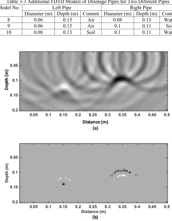
For illustration purposes, three additional models are presented where the two pipes have different conditions. Detailed parameters are shown in Table 3-3. The thresholds of left and right pipes are different, so step 4 of the migration algorithm was not performed. The same numerical estimations of pipe diameter and depth used in the aforementioned models were used in these three additional models.
Figure 3-10 shows that the left pipe has positive pixel values, while the right pipe has large negative pixel values. This suggests that the left pipe is empty, while the right pipe is filled with water. The pipe on the left has a smaller diameter and a larger depth. Similarly, the left pipe has positive pixel values and the right pipe has small negative pixel values (Figure 3-11). This suggests that the left pipe is empty, while the right pipe is filled with soil. Again, the pipe on the left has a smaller diameter and a larger depth. On the other hand, Figure 3-12 shows both pipes having negative pixels. The left one has a smaller absolute value, indicating it is filled with soil, while the right pipe is filled with water.
Table 3-3 Additional FDTD Models of Drainage Pipes for Two Different Pipes
Model No. Left Pipe Right Pipe
Diameter (m) Depth (m) Content Diameter (m) Depth (m) Content
8 0.06 0.15 Air 0.08 0.13 Water
9 0.06 0.15 Air 0.1 0.11 Soil
10 0.08 0.13 Soil 0.1 0.11 Water
Figure 3-10 Reconstructed image of Model 8: (a) Migration reconstruction, and (b) sparse reconstruction.
Figure 3-11 Reconstructed image of Model 9: (a) Migration reconstruction, and (b) sparse reconstruction.
Figure 3-12 Reconstructed image of Model 10: (a) Migration reconstruction, and (b) sparse reconstruction.
3.5 Summary
In this chapter, the generic GPR imaging theory was discussed, and the forward imaging problem was demonstrated to be a linear problem under certain assumptions. Two linear inversion techniques were then developed, including migration and sparse reconstruction.
The FDTD simulation theory was described and an example of drainage pipe simulation was conducted. The simulated drainage models showed different condition parameters including
locations, diameters, and contents. The proposed two image reconstruction techniques were then applied to the simulated GPR signal to reconstruct the drainage pipes under concrete pavement. The depth, diameter, and content of the drainage pipes were then estimated based on the reconstructed targets. The findings can be summarized as follows:
1) Both migration and sparse reconstruction can reconstruct 2-D targets when the linearity assumptions are met.
2) For drainage pipe reconstruction, both migration and sparse reconstruction can only reconstruct the top surface of the drainage pipes. This is due to the violation of the linearity assumption in GPR imaging.
3) SPG algorithm can be used to efficiently solve the LASSO problem.
4) Migration algorithms can effectively reconstruct the target, but require manually selecting a proper threshold. The drainage pipes content can be estimated based on the migration-reconstructed image.
5) Sparse reconstruction is more accurate than the migration algorithm, but it requires more computation time than the migration algorithm. The size and location of the drainage pipes can be accurately estimated based on the sparse reconstruction results.
In practice, migration better detects the presence of the drainage pipes and more efficiently estimates the content of the drainage pipes; the sparse reconstruction better estimates the location and size of the drainage pipes quantitatively.
As a continuation of the study, the recommendations for future studies are as follows: 1) The performance of both reconstruction methods need to be validated on real GPR signals
collected from underground targets.
3) Reconstruction performance with different pavement structures, such as layered structures, needs to be studied.
4)
Potential interference due to close proximity of targets need to be considered.This chapter explains the general GPR imaging problem. Starting from here, the thin AC overlay thickness and density estimation problem can be solved using methods similar to those used for the two image reconstruction.
CHAPTER 4: DEVELOPMENT OF REGULARIZATION METHODS ON
SIMULATED GPR SIGNALS TO PREDICT THIN AC OVERLAY
THICKNESS
4.1 Background and Objective
This chapter presents the details of one of the proposed approaches to find thin AC overlay thickness, regularization method. The range resolution of GPR antenna signal is an important parameter in thin asphalt overlay thickness estimation. When the asphalt pavement thickness is comparable to the EM wavelength of the GPR signal, the GPR reflection from the pavement surface and the bottom of the surface layer may overlap. In such cases, our goal is to increase the resolution of the GPR signal, such that the reflections can be individually resolved.
In section 4.2, we’ll first develop a mathematical model for GPR survey on two layered AC pavement, and then propose the four types of regularization algorithms, including Tikhonov regularization and total variation regularization. In section 4.3, the four regularization methods will be applied on simulated noisy GPR signals, and their performance will be evaluated. Section 4.4 summarizes this chapter.
4.2 Algorithm Development
4.2.1 Mathematical model
In this study, we consider two-layered AC pavement as shown in Figure 2-4, where the first layer is the surface binder, which is the thin overlay, and the second layer is the leveling binder, which could also be the old pavement. Here we assume that the reflection coefficient at ground surface, −𝐴L/𝐴`, is negative, and that the reflection coefficient at bottom of the surface binder, −𝐴U/𝐴`, is positive, as with the red arrows shown in Figure 2-4. The incident signal is Ricker wavelet type. 𝐴L, 𝐴U, and 𝐴` are the reflection amplitude from the pavement surface, the bottom
A linear time-invariant system is a system that satisfies the following two properties:
• Linearity: a linear combination of the input will result in the linear combination of the corresponding outputs. For example, if the input 𝑥L(𝑡) produces output 𝑦L(𝑡), and input 𝑥U(𝑡) produces output 𝑦U(𝑡), then 𝑎L𝑥L(𝑡) + 𝑎U𝑥U(𝑡) produces output 𝑎L𝑦L(𝑡) + 𝑎U𝑦U(𝑡), where 𝑎L and 𝑎U are real scalars.
• Time-invariance: if we delay the input by some time interval, the output will be delayed by the same amount of time. For example, if 𝑥L(𝑡) produces output 𝑦L(𝑡), then 𝑥L(𝑡 + Δ𝑡) produces output 𝑦L(𝑡 + Δ𝑡).
It is easy to see that under the assumptions that AC is homogeneous, non-dispersive, and isotropic material, the asphalt pavement shown in Figure 2-4 is a linear time-invariant system: the input is the incident signal while the output is the GPR signal reflected from the pavement structure.
For a linear time-invariant system, the output signal is the convolution of the input signal and the system impulse response. In our case, the output signal y(t) is the convolution of incident signal x(t) and the pavement system impulse response h(t):
𝑦(𝑡) = ℎ(𝑡) ∗ 𝑥(𝑡) = £ ℎ(𝑡 − 𝑢)𝑥(𝑢)𝑑𝑢 ¦
9
, (4-1)
where y(t) is the pavement reflection signal, x(t) is the incident signal (usually Ricker wavelet), and h(t) is the impulse response. For a layered pavement system, h(t) simply consists of impulses at each layer interface, with amplitudes equal to the reflection coefficient at each layer interface, as shown by the red arrows in Figure 2-4. The impulse response h(t) contains the information we are interested in: the TWTT and the surface reflection amplitude. Therefore, we’ll be able to calculate the asphalt overlay thickness and density once the impulse response is known. For GPR
application, y(t) and x(t) are known from the pavement reflection and the copper plate reflection, while h(t) is unknown.
4.2.2 GPR signal resolution
If the pavement is thick, we will identify the reflection from the asphalt pavement surface and the bottom of the surface layer, and directly obtain the two-way travel time and surface reflection coefficient without any signal processing techniques. However, as stated in the “problem statement” section, when the layer thickness is thin compared to EM wavelength, the two pulses shown in Figure 2-4 will overlap with each other. Figure 4-1 illustrates this thin layer challenge.
Figure 4-1 shows the simulated output signal from a two-layer asphalt pavement model with different thicknesses. The incident signal in the simulation is the same as the one used by air-coupled antenna in this study. The incident signal is a Ricker wavelet with an arbitrary amplitude and an EM wavelength duration of 0.5382 ns. The dashed lines show the GPR signals which are generated by convoluting the incident GPR signal with Dirac delta functions at the surface and the bottom of the asphalt pavement layer. The amplitude of the Dirac delta functions represents the reflection coefficient that can be used to calculate the dielectric constant for each layer. The sign of impulses in Figure 4-1 are intentionally inverted for visualization purposes. For example, an impulse amplitude of the surface reflection of 0.3 means that 𝐴L/𝐴`= −0.3; therefore, the dielectric constant 𝜀L is 3.45, as calculated by equation 2-12. The locations and amplitudes of the Dirac delta function are simply assumed by the authors for the purpose of demonstration.
Figures 4-1(a) through 4-1(f) show the increase in layer thickness from 0.71 times the wavelength to 1.79 times the wavelength. For the Ricker wavelet-type of incident signal used in this study, the length of the wavelet is around twice the length of the EM wavelength. Figures 4-1(c), 4-1(d), 4-1(e) and 4-1(f) show that the two peaks can be seen directly because the thickness
is relatively large; however, Figures 4-1(a) and 4-1(b) show that the second reflection is masked by the surface reflection, resulting in difficulties in obtaining the two-way travel time.
The two solid vertical lines in each figure represent the inverse of the assumed impulse responses at each layer interface. The amplitudes of these two impulses are −𝐴L and −𝐴U, respectively, as shown in Figure 2-4. In Figure 4-1, the amplitude of the impulse responses is magnified to better show the locations of the surface and the bottom of the asphalt pavement layer.
Figure 4-1 Pavement reflection (dashed) and impulse response (solid) for layer thickness which
is a) 0.71 b) 0.93 c) 1.14 d) 1.36 e) 1.57 f) 1.79 times of the EM wavelength.
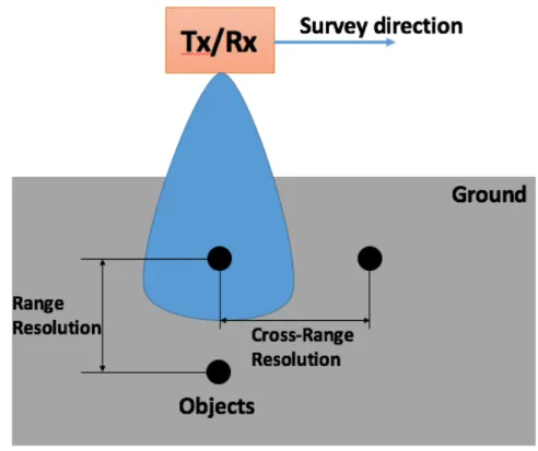
Thin layers present a challenge because GPR signals lack adequate range resolution. Radar resolution is an importation parameter for imaging (Soumekh 1999). The cross-range resolution (or azimuth resolution) of a radar describes its ability to resolve targets that are closely placed in angle, while the range resolution describes its ability to resolve targets closed placed in the range direction. This is shown in Figure 4-2, in which the round black circle represents general
underground targets, such as rebar, drainage pipes, landmines, archaeological structures, and layered pavement. The cross-range resolution of a radar is usually determined by its antenna pattern: the larger the directivity of the antenna, the better the cross-range resolution. An example of the GPR antenna pattern is represented by the blue area shown in Figure 4-2. The range resolution of a radar is determined by the bandwidth of the antenna. Signals with a wider bandwidth have shorter pulse durations, allowing for target resolution at a closer distance. In extreme cases, signals of infinite bandwidth become impulse signals (or Dirac Delta functions) and have perfect range resolution. In practice, all signals are band-passed signals, and therefore have a nonzero pulse duration.
Figure 4-2 Illustration of range resolution and cross-range resolution of GPR
In the application of measuring asphalt layer thickness, whether using the conventional two-way travel time method or the XCMP method, the key factor determining GPR performance
which only varies in the vertical direction. Thus, it is preferable to use wide band antennas (e.g., horn antennas) or ultra-wide band antennas (e.g., bow-tie antennas) as GPR antennas (Stutzman and Thiele 2012).
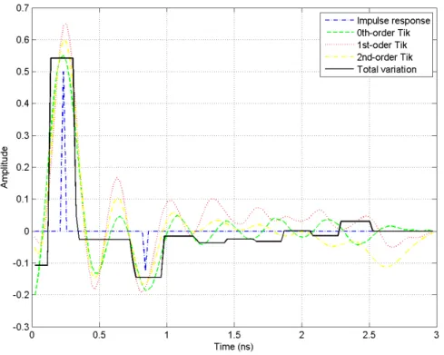
There are many ways to characterize the range resolution of a signal. The most common method is to use Rayleigh resolution criteria (Culick 1987). The Rayleigh resolution Δ𝑡§¨B©kª«¬ of a one dimensional signal is defined as the distance between the maximum point of a pulse and the first diffraction minimum of that pulse. Figure 4-3 depicts the situations when the two identical GPR pulses are resolved at the exact distance of Rayleigh resolution and unresolved, respectively. For pulses with a particular shape, their Rayleigh resolution 𝐵Δ𝑡§¨B©kª«¬ is inversely proportional to the bandwidth of the pulse, 𝐵, or 𝐵Δ𝑡§¨B©kª«¬= 𝑐𝑜𝑛𝑠𝑡. Rayleigh resolution is one of the many factors that determine the ability to resolve closely spaced pulses—other factors include the shape of the pulse, the amplitude ratio of the adjacent pulses, and the signal to noise ratio (SNR) of the signal, etc. For GPR antennas with a 2GHz center frequency, if the pavement has a dielectric constant of 9, the EM wave predominant wavelength is 5 cm. While the Rayleigh resolution is about half of the predominant wavelength, 2.5cm, the practical resolution is about one quarter of the predominant wavelength, 1.25cm (Kallweit and Wood 1982). For thin asphalt overlay thickness estimation this is less certain, since the reflection from the bottom of the asphalt overlay is generally small, as shown in Figure 4-1, due to the similarity of the dielectric constants of the asphalt overlay and the old pavement. This suggests that it is much more difficult to resolve thin layers, as in the case of asphalt pavement. It should be noted that the unit of the vertical amplitude axis is normalized voltage. The absolute amplitude value is not critical since in this study we always use the amplitude ratio for calculating the dielectric constant. This is true throughout the dissertation.
Figure 4-3 Demonstration of Rayleigh resolution of typical GPR signal: red signal is surface reflection, yellow signal is bottom reflection, and blue signal is total reflection.
4.2.3 Tikhonov regularization
Due to physical restrictions, the bandwidth of GPR antennas have an upper limit; thus, signal processing techniques are needed to increase the range resolution. These are called super-resolution techniques. One of the most common is the “layer stripping” method (Spagnonili, 1997), in which reflections are detected by a matched filter detector and then iteratively subtracted from the original signal. This method has been successfully applied to asphalt layer thickness detection (Lahour and Al-Qadi, 2008). The main drawback of this approach is that it is not robust to noises, resulting in large errors in amplitude and dielectric constant detection. An alternative to the layer stripping approach is the linear inversion technique, which we will discuss in this chapter.
Our goal is now to recover the ℎ(𝑡) from equation (4-1). Since real world electronic signals are all continuous in time, the first step is to discretize equation (4-1) such that it can be processed by computer. When the Nyquist criterion is met, we can uniformly sample x(t), y(t) and h(t) to transform Equation (4-1) into:
where 𝑦⃗ ∈ ℂ(d–•uL)×L and ℎ#⃗ ∈ ℂ•×L are vectors of y(t) and h(t), 𝑿 ∈ ℂ(d–•uL)ו is the Toeplitz matrix constructed from 𝑥⃗, the vector by sampling x(t). Here m and n are the dimensions of 𝑥⃗ and ℎ#⃗, respectively. It should be noted that, technically, 𝑥⃗, 𝑦⃗, and ℎ#⃗ should have infinite lengths due to x(t), y(t) and h(t), but here we ignore the starting and ending zeroes, making the three vectors finite in length. Our problem now is to find the impulse response ℎ#⃗ from 𝑦⃗ and 𝑿. This is a linear inversion problem: finding ℎ#⃗r that can approximate ℎ#⃗.
Following the general GPR image reconstruction theory introduced in Chapter 3.3, there are two types of inversing techniques for the reconstruction of one-dimensional targets (here, asphalt pavement layers): matched filtering and deconvolution. These correspond to migration and inverse filtering techniques employed in general GPR image reconstruction (Soumekh 1999).
The matched-filtering technique is commonly used for chirp signals; i.e., linearly frequency-modulated (FM) signals. However, matched-filtered signals may not resolve pulsed signals (Soumekh 1999). The deconvolution method is a signal processing technique that can in theory perfectly resolve the target location (Riad 1986). For linear FM signals, it can be demonstrated that the matched-filter gives the same result as the deconvolution method. The forward and inverse models of one-dimensional GPR imaging for matched-filter and deconvolution are illustrated in Figure 4-4.
As shown in Figure 4-4, we consider h(t) to be the input signal instead of x(t). This is feasible since convolution is commutable: h(t) is first convolved with x(t) to get output y(t). For the matched-filtering method, 𝑦(𝑡) is filtered by 𝑥∗(−𝑡), where 𝑥∗(𝑡) is the complex conjugate of 𝑥(𝑡). Matched filtering is essentially the auto-correlation of signal 𝑥(𝑡). For the deconvolution method, 𝑦(𝑡) is filtered by 𝐹uL² L
³(´)µ, where 𝐹
uL represents the inverse Fourier transform, and
Fourier transform of 1/X(ω), as shown in Figure 4-4, is usually not applicable in practice because X(ω) is typically band-limited. Alternatively, the time domain deconvolution can be done by regularization, as illustrated in the following section.
Figure 4-4 1-D target reconstruction: matched filtering and deconvolution.
The matched-filter technique has been used in GPR applications (Leuschen and Plumb 2001). To increase the range resolution of GPR signals, Savelyev and Sato (2004) report the success of the deconvolution method in landmine detection. Al-Qadi and Lahouar (2005) also report good results in estimating asphalt pavement layer thickness using the deconvolution method. Economou et al. (2012) and Schmelzbach et al. (2015) developed several deconvolution algorithms on GPR signals. However, none of these studies concern the ill-posed nature of the deconvolution.
The authors (Zhao et al. 2015) proposed a regularized deconvolution method and applied it on field data, with promising results. Regularizing the deconvolution makes it more robust to noise and small amplitude reflections, such as reflection at asphalt pavement layer interfaces. However, Zhao et al. (2015) only consider zeroth-order Tikhonov regularization, and the influence of noise levels and layer thickness on the performance of the deconvolution algorithm was not discussed.