buildings
ArticleImage Post-Processing Method for Quantification of
Cracking in RC Precast Beams under Bending
Albert Albareda-Valls *, Alejandra Bustos Herrera , Joan Lluís Zamora Mestre and Saeid S. Zaribaf
School of Architecture, Department of Technology in Architecture, Polytechnic University of Catalunya, Av Diagonal 649, 08034 Barcelona, Spain; [email protected] (A.B.H.);
[email protected] (J.L.Z.M.); [email protected] (S.S.Z.) * Correspondence: [email protected]; Tel.: +34-639-523-624
Received: 16 August 2018; Accepted: 30 October 2018; Published: 13 November 2018
Abstract: Image processing methods are increasingly used in civil engineering, especially in the maintenance of concrete structures. Current digital cameras and post-processing methods allow verifying qualitatively the state of conservation of wide areas of concrete in dams and bridges. When dealing with building refurbishments and rehabilitation, it is important to verify that existing structural elements fit the requirements of the standards; in the case of structures formed by traditional RC joists, cracking of the bottom-face provides information about the serviceability of these elements. This research proposed and put in practice through experimental tests an image post-processing method for quantification of cracking (five specimens were used and calibrated). Based on a sequence of shots and through a complex step-by-step post-processing, cracks were identified and measured to calibrate this method for real purposes. The method quantifies the crack opening width and spacing by analyzing the bottom-face of the joists through the shots. Measured values of crack spacing are very similar to those predicted by the standards, while the values of crack opening width differ more from theoretical ones due to the scattering of results. However, the proposed method has been proved as suitable and useful for fast inspections of RC elements under bending.
Keywords:image-based analysis; crack detection; serviceability; durability
1. Introduction
Image-based analysis methods are becoming usual procedures to examine constructive elements due to the big amount of information they can provide with a single shot. High-resolution images may detect even small details, such as cracks or spots on a regular predefined surface. This becomes very useful, especially when these irregularities are almost invisible by humans, to determine specific conditions of degradation of concrete elements in civil structures [1]. Worldwide governments and authorities push to extend the use of these methods on bridges and dams, due to the difficulties in carrying out regular inspections [1–3].
Up to date, the common method to carry out the maintenance of civil infrastructure systems is based on visual inspections. This procedure is clearly not efficient from all points of view, and may lead to overlook serious incidences affecting concrete. Under this assumption, automated non-destructive inspection methods become strong candidates to overcome the shortcomings thanks to being independent of the human being criterion.
However, these methods have only been put in practice for maintenance issues involving concrete, which is the main challenge for civil authorities in the next decades. Only few existing studies have used these procedures to quantify or evaluate mechanical behaviors. In architectural RC structures, the standards allow certain cracks on concrete in slabs and beams subjected under bending.
Buildings2018,8, 158 2 of 21
The main goal of this research was to propose and put in practice an image-based post-processing method to quantify the crack opening width (therefore, the loading state) of traditional precast RC joists subjected to pure bending. RC traditional joists have been chosen to conduct this research due to their sensitivity to get cracked under low-bearing bending, although it could be extended to any RC element by knowing its geometry and strengths. The method proposes an image-based analysis of the cracking pattern at the bottom-face of RC joists: cracks reveal significant information, including about the loading conditions. The possibility of determining the real loading status becomes a very interesting issue, especially for refurbishment and consolidation works. This research puts in practice a new method through real cracks on RC joists to use it for real purposes. Traditional RC joists (without pre-stressing) are commonly used in Northern Spain for housing made of one-way slabs up to 5-m span (see Figure1).
Buildings 2018, 8, x FOR PEER REVIEW 2 of 21
structures, the standards allow certain cracks on concrete in slabs and beams subjected under bending.
The main goal of this research was to propose and put in practice an image-based post-processing method to quantify the crack opening width (therefore, the loading state) of traditional precast RC joists subjected to pure bending. RC traditional joists have been chosen to conduct this research due to their sensitivity to get cracked under low-bearing bending, although it could be extended to any RC element by knowing its geometry and strengths. The method proposes an image-based analysis of the cracking pattern at the bottom-face of RC joists: cracks reveal significant information, including about the loading conditions. The possibility of determining the real loading status becomes a very interesting issue, especially for refurbishment and consolidation works. This research puts in practice a new method through real cracks on RC joists to use it for real purposes. Traditional RC joists (without pre-stressing) are commonly used in Northern Spain for housing made of one-way slabs up to 5-m span (see Figure 1).
(a) (b)
Figure 1. Reinforced RC joists (without pre-stressing) are commonly used in northern Spain areas: (a) lateral view of typical RC joists; and (b) general view of the one-way ribbed slabs, source: Iberaceros Forjados Riojanos, [4].
Image-based existing tools are enough accurate to obtain all the necessary data from the shots to be easily processed. Using this, the loading status and the damage ratio of one-way slabs may be quickly evaluated thanks to the help of a camera.
2. State of the Art
2.1. Image-Based Analysis for Construction
Several researchers have been working in implementing crack detection through image-based analysis on concrete elements [5,6]; most of these studies deal with durability of concrete and they do not use this technology for other mechanical purposes. For instance, Porras et al. [7] proposed a specific method to detect the spreading of traverse cracks in concrete pavements. Abdel-Qader et al. [3] used images to identify cracks and the state of conservation of pavements in bridges, and proposed algorithms for crack patterns in pavements of bridges. Benning et al. [8] used photogrammetry to measure reinforced concrete deformations and monitor cracks.
More recent is the research done by Jahanshahi et al. [9], who evaluated several image-based techniques with real infrastructures. Fujita and Namamoto [10] proposed a crack detection method in noisy concrete surfaces using probabilistic relaxation. Zhu et al. [11] composed a method to establish crack properties such as length, orientation or width to determine the damage caused by earthquakes on reinforced concrete structures. Jahanshahi et al. [12] provided a specific methodology to analyze cracks using images from any distance, focus or resolution.
Figure 1.Reinforced RC joists (without pre-stressing) are commonly used in northern Spain areas: (a) lateral view of typical RC joists; and (b) general view of the one-way ribbed slabs, source: Iberaceros Forjados Riojanos, [4].
Image-based existing tools are enough accurate to obtain all the necessary data from the shots to be easily processed. Using this, the loading status and the damage ratio of one-way slabs may be quickly evaluated thanks to the help of a camera.
2. State of the Art
2.1. Image-Based Analysis for Construction
Several researchers have been working in implementing crack detection through image-based analysis on concrete elements [5,6]; most of these studies deal with durability of concrete and they do not use this technology for other mechanical purposes. For instance, Porras et al. [7] proposed a specific method to detect the spreading of traverse cracks in concrete pavements. Abdel-Qader et al. [3] used images to identify cracks and the state of conservation of pavements in bridges, and proposed algorithms for crack patterns in pavements of bridges. Benning et al. [8] used photogrammetry to measure reinforced concrete deformations and monitor cracks.
More recent is the research done by Jahanshahi et al. [9], who evaluated several image-based techniques with real infrastructures. Fujita and Namamoto [10] proposed a crack detection method in noisy concrete surfaces using probabilistic relaxation. Zhu et al. [11] composed a method to establish crack properties such as length, orientation or width to determine the damage caused by earthquakes on reinforced concrete structures. Jahanshahi et al. [12] provided a specific methodology to analyze cracks using images from any distance, focus or resolution.
Buildings2018,8, 158 3 of 21
2.2. Constitutive Behavior of Concrete
Concrete is a cohesive material which behaves differently under tension than under compression; as is well-known, although the response of the material is ductile-like under compression (see Figure2), it is clearly fragile under tension [13]. Besides, its capacity under tension only reaches a mean of 9% of its strength under compression, and this is the reason concrete elements such as beams or slabs need to be reinforced with steel rebars. This is the reason reinforced concrete describes complex nonlinearities due to a constant variation of the cracked area of the cross-section.
Buildings 2018, 8, x FOR PEER REVIEW 3 of 21
2.2. Constitutive Behavior of Concrete
Concrete is a cohesive material which behaves differently under tension than under compression; as is well-known, although the response of the material is ductile-like under compression (see Figure 2), it is clearly fragile under tension [13]. Besides, its capacity under tension only reaches a mean of 9% of its strength under compression, and this is the reason concrete elements such as beams or slabs need to be reinforced with steel rebars. This is the reason reinforced concrete describes complex nonlinearities due to a constant variation of the cracked area of the cross-section.
Figure 2. Uniaxial stress-strain curve for plain concrete. Source: [14].
Under high ratios of compressive and tensile loading, concrete starts being affected by a reduction of stiffness; this phenomenon is known as constitutive damage. On the one hand, the evolution of damage under compression forces is basically due to micro-crushing of the material, leading to a clear ductile response. On the other hand, the evolution of damage under tension is caused by crack propagation, a fact that leads to a fragile response through a sharp collapse.
2.3. Bending Response of RC Elements
When reinforced concrete (RC) elements are subjected to pure bending, compression and tension stresses appear along the cross-section: while upper fibers of the section become mainly compressed, bottom-fibers become proportionally subjected to tension until reaching the concrete tensile strength; beyond this point, steel reinforcements are needed. Reinforcements let the section reach the ultimate plastic bending moment, but also help to minimize the opening width of cracks in concrete. Under these assumptions, cracks always appear at the bottom-face of bended elements; thus, by knowing the geometry of the section, the size and spacing of cracks tells about the magnitude of loading.
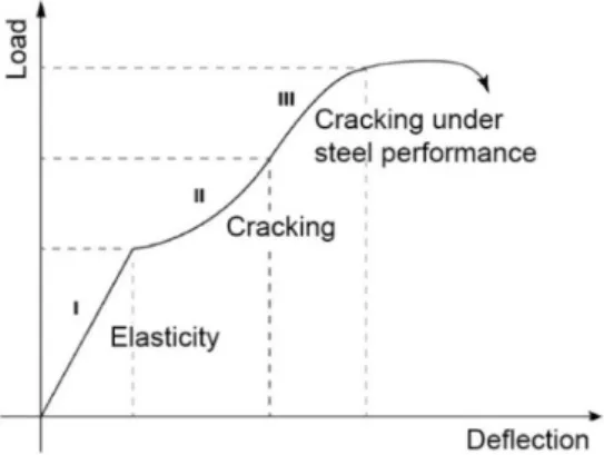
As it has been previously mentioned, cracks appear when the first bottom-fiber of the cross-section reaches the maximum concrete tensile strength. Before this point, the behavior of concrete is mostly linear (Phase I in Figure 3). Once cracking takes place, the section is increasingly affected by a reduction of area, together with the increment of load that leads to a nonlinear behavior as cracks get bigger (Phase II in Figure 3). Phase III (Figure 3) is achieved when stability of the whole section only depends on reinforcing bars, as concrete becomes completely cracked below the neutral axis; at that point, nonlinearity response is significant and leads directly to the final collapse.
Although cracks on the bottom-face of a RC joist are commonly permissible, the truth is that, in the case of becoming significantly wide, the process of oxidation may be accelerated and finally influence the durability of reinforcements; this is the reason most codes and regulations provide analytical methods to quantify the opening width by establishing a maximum value of 0.2 mm [14,15]. To summarize, crack opening width on RC elements provides information about the loading status if geometry and reinforcements are known.
Figure 2.Uniaxial stress-strain curve for plain concrete. Source: [14].
Under high ratios of compressive and tensile loading, concrete starts being affected by a reduction of stiffness; this phenomenon is known as constitutive damage. On the one hand, the evolution of damage under compression forces is basically due to micro-crushing of the material, leading to a clear ductile response. On the other hand, the evolution of damage under tension is caused by crack propagation, a fact that leads to a fragile response through a sharp collapse.
2.3. Bending Response of RC Elements
When reinforced concrete (RC) elements are subjected to pure bending, compression and tension stresses appear along the cross-section: while upper fibers of the section become mainly compressed, bottom-fibers become proportionally subjected to tension until reaching the concrete tensile strength; beyond this point, steel reinforcements are needed. Reinforcements let the section reach the ultimate plastic bending moment, but also help to minimize the opening width of cracks in concrete. Under these assumptions, cracks always appear at the bottom-face of bended elements; thus, by knowing the geometry of the section, the size and spacing of cracks tells about the magnitude of loading.
As it has been previously mentioned, cracks appear when the first bottom-fiber of the cross-section reaches the maximum concrete tensile strength. Before this point, the behavior of concrete is mostly linear (Phase I in Figure3). Once cracking takes place, the section is increasingly affected by a reduction of area, together with the increment of load that leads to a nonlinear behavior as cracks get bigger (Phase II in Figure3). Phase III (Figure3) is achieved when stability of the whole section only depends on reinforcing bars, as concrete becomes completely cracked below the neutral axis; at that point, nonlinearity response is significant and leads directly to the final collapse.
Although cracks on the bottom-face of a RC joist are commonly permissible, the truth is that, in the case of becoming significantly wide, the process of oxidation may be accelerated and finally influence the durability of reinforcements; this is the reason most codes and regulations provide analytical methods to quantify the opening width by establishing a maximum value of 0.2 mm [14,15].
Buildings2018,8, 158 4 of 21
To summarize, crack opening width on RC elements provides information about the loading status if geometry and reinforcements are known.Buildings 2018, 8, x FOR PEER REVIEW 4 of 21
Figure 3. Typical load-deflection diagram of a reinforced concrete beam under bending. Source: [13] 3. Cracking according to Eurocode 2
Several approaches can be found among literature to evaluate the evolution of cracking in RC elements under bending. Borosnyòi and Balàzs [16] in their state-of-the-art study on cracking of RC elements reported the difficulties of determining the two more relevant parameters in cracking: the mean crack width and spacing. Allam et al. [17] concluded their research by assuming that the opening crack width and spacing are both parameters that show a significant scatter among results, although Eurocode 2 and ACI approaches provided quite good agreement with reality. Values from these two methods show a better accuracy rather than other methods like the one provided by the British Standards. This is the reason the Eurocode 2 approach has been chosen to predict the theoretical values corresponding to tested specimens, due to the difficulty in getting a mean value of the opening crack width experimentally. Thus, the accuracy of the proposed method derives from the accuracy of Eurocode 2 (which is well-calibrated). The expression which is proposed by the standard to calculate the characteristic crack width is the following:
𝑤 = 𝑆, (𝜀 − 𝜀 ) (1)
𝑤 is ths characteristic crack width; 𝑆, is the maximum crack distance; and (𝜀 − 𝜀 ) is the difference in deformation between steel and concrete over the maximum crack distance.
The difference in deformation can be calculated by using the following expression:
(𝜀 − 𝜀 ) = 𝜎 − 𝑘 ·𝑓𝜌 , , · (1 + 𝛼 · 𝜌 , ) 𝐸 ≥ 0,6 𝜎 𝐸 (2)
where 𝜎 is the stress in the steel assuming a cracked section; 𝛼 is the moduli ratio 𝐸 𝐸⁄ ; 𝐸 is the elastic modulus of steel; 𝑓 , is the mean tension strength of concrete when cracking takes place; 𝜌 , = is the effective reinforcement ratio; 𝜉 — 𝜉 ·∅∅ —𝜉 is the ratio of bond strength of prestressing and reinforcing steel; ∅ is the largest bar diameter of reinforcing steel; ∅ is the equivalent diameter of tendon; 𝑘 is a factor depending on the duration of load (0.6 for short and 0.4 for long term loads); 𝐴 is the minimum steel area in the tensile zone; and 𝐴 is the area of pre or post-tensioned tendons within the effective area of concrete cross-section.
The maximum final crack spacing can be calculated using Clause 7.3.4 (Equations (7) and (11)):
𝑆, = 𝑘 · 𝑐 + 𝑘 · 𝑘 · 𝑘 ·𝜌𝜙
, (3)
where 𝑐 is the concrete cover; 𝜙 is the bar diameter; 𝑘 is the bond factor (0.8 for high bars, 1.6 for bars with an effectively plain surface); 𝑘 is the strain distribution coefficient (1.0 for tension and 0.5 for bending; 𝑘 is recommended to be 3.4; and 𝑘 is recommended to be 0.425.
Figure 3.Typical load-deflection diagram of a reinforced concrete beam under bending. Source: [13] 3. Cracking according to Eurocode 2
Several approaches can be found among literature to evaluate the evolution of cracking in RC elements under bending. Borosnyòi and Balàzs [16] in their state-of-the-art study on cracking of RC elements reported the difficulties of determining the two more relevant parameters in cracking: the mean crack width and spacing. Allam et al. [17] concluded their research by assuming that the opening crack width and spacing are both parameters that show a significant scatter among results, although Eurocode 2 and ACI approaches provided quite good agreement with reality. Values from these two methods show a better accuracy rather than other methods like the one provided by the British Standards. This is the reason the Eurocode 2 approach has been chosen to predict the theoretical values corresponding to tested specimens, due to the difficulty in getting a mean value of the opening crack width experimentally. Thus, the accuracy of the proposed method derives from the accuracy of Eurocode 2 (which is well-calibrated). The expression which is proposed by the standard to calculate the characteristic crack width is the following:
wk=Sr,max(εsm−εcm) (1)
wk is ths characteristic crack width; Sr,max is the maximum crack distance; and (εsm−εcm) is the difference in deformation between steel and concrete over the maximum crack distance.
The difference in deformation can be calculated by using the following expression:
(εsm−εcm) = σs−kt· fct,e f f ρp,e f f· 1+αe·ρp,e f f Es ≥0.6σs Es (2)
whereσsis the stress in the steel assuming a cracked section;αeis the moduli ratioEs/Ecm;Esis the elastic modulus of steel; fct,e f f is the mean tension strength of concrete when cracking takes place; ρp,e f f = (
As+ξ1Ap)
Ap is the effective reinforcement ratio;ξ1— q
ξ·∅s
∅p—ξis the ratio of bond strength of prestressing and reinforcing steel;∅s is the largest bar diameter of reinforcing steel; ∅p is the equivalent diameter of tendon;ktis a factor depending on the duration of load (0.6 for short and 0.4 for long term loads);Asis the minimum steel area in the tensile zone; andApis the area of pre or post-tensioned tendons within the effective area of concrete cross-section.
The maximum final crack spacing can be calculated using Clause 7.3.4 (Equations (7) and (11)): Sr,max =k3·c+k1·k2·k4·
φ ρp,e f f
Buildings2018,8, 158 5 of 21
wherecis the concrete cover;φis the bar diameter;k1is the bond factor (0.8 for high bars, 1.6 for bars with an effectively plain surface);k2is the strain distribution coefficient (1.0 for tension and 0.5 for bending;k3is recommended to be 3.4; andk4is recommended to be 0.425.
To apply the crack width expressions, basically established for a concrete bar in tension, to a structure under bending, a definition of the “effective tensile bar height” is necessary. This effective heighthc,e f f can be determined though Figure4.
Buildings 2018, 8, x FOR PEER REVIEW 5 of 21
To apply the crack width expressions, basically established for a concrete bar in tension, to a structure under bending, a definition of the “effective tensile bar height” is necessary. This effective height ℎ , can be determined though Figure 4.
Figure 4. Effective height, hc,eff according to Eurocode 2 [13]. 𝐴, level of steel centroid; 𝐵, effective
tensioned area Ac,eff.
4. Experimental Campaign
To put in practice the suitability of the proposed image post-processing method to determine the loading and cracking status of RC elements under bending, an experimental campaign was carried out: five single RC traditional joists were subjected to a four-point bending test. All suffered from typical cracking patterns on the bottom-face. By following the same steps of loading, the sequence of cracks was photographed with high-resolution shots by fixing the camera totally perpendicular to specimens.
The purity of a four-point bending test leads to uniform crack patterns which allow comparing the values of cracks measured from pictures with those analytically predicted. Once the pattern and the crack opening width are faithfully determined by the image post-processing method, the loading status may be also easily correlated.
4.1. Tested Specimens
Five single RC prefabricated joists of 125 mm × 45 mm cross-section (V1–V5, see Figure 5) were tested under pure bending at laboratory, according to the requirements of the standards for pure bending tests. All specimens were made of 25 MPa strength concrete, reinforced with three 6 mm-bar of 500 MPa steel; slight differences regarding the distribution of reinforcements were considered for each specimen, similar to under real conditions. Specimens were kindly provided by Forjados Orgues SL, from Murchante (Northern Spain) [4], as these elements are commonly used in these areas for housing. Since this typology of joists are not pre-stressed, deflections and cracking use to reach significant values under low bearing conditions.
Figure 4.Effective height, hc,effaccording to Eurocode 2 [13]. A, level of steel centroid;B, effective tensioned areaAc,eff.
4. Experimental Campaign
To put in practice the suitability of the proposed image post-processing method to determine the loading and cracking status of RC elements under bending, an experimental campaign was carried out: five single RC traditional joists were subjected to a four-point bending test. All suffered from typical cracking patterns on the bottom-face. By following the same steps of loading, the sequence of cracks was photographed with high-resolution shots by fixing the camera totally perpendicular to specimens. The purity of a four-point bending test leads to uniform crack patterns which allow comparing the values of cracks measured from pictures with those analytically predicted. Once the pattern and the crack opening width are faithfully determined by the image post-processing method, the loading status may be also easily correlated.
4.1. Tested Specimens
Five single RC prefabricated joists of 125 mm×45 mm cross-section (V1–V5, see Figure5) were tested under pure bending at laboratory, according to the requirements of the standards for pure bending tests. All specimens were made of 25 MPa strength concrete, reinforced with three 6 mm-bar of 500 MPa steel; slight differences regarding the distribution of reinforcements were considered for each specimen, similar to under real conditions. Specimens were kindly provided by Forjados Orgues SL, from Murchante (Northern Spain) [4], as these elements are commonly used in these areas for housing. Since this typology of joists are not pre-stressed, deflections and cracking use to reach significant values under low bearing conditions.
Buildings2018,8, 158 6 of 21
Buildings 2018, 8, x FOR PEER REVIEW 6 of 21
Figure 5. Tested typical RC joist specimens, provided by Forjados Orgues. 4.2. Features of the Test
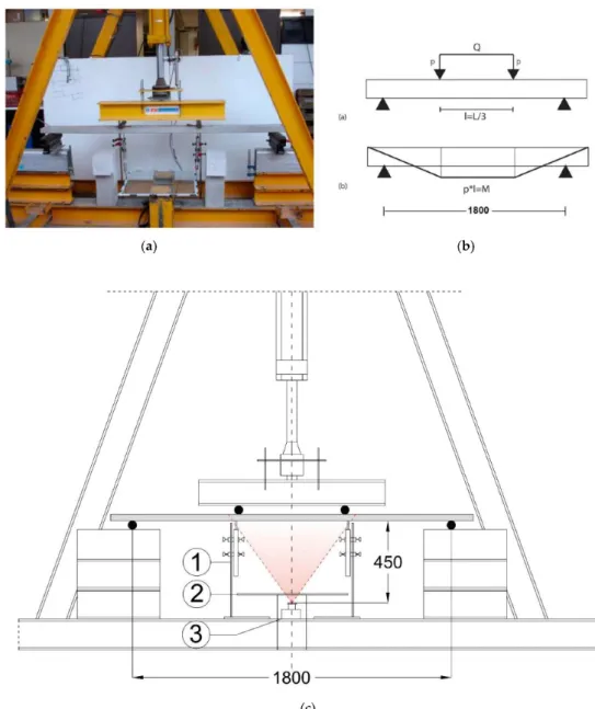
The carried-out test consists in a simple four-point bending test, according to Eurocode (Figure 6). A 10-Ton activator pushing on a rigid steel profile distributes the load uniformly into two separated points on specimens. This way, the length between the two loading points becomes subjected to pure bending, so that that the pattern of cracks results totally uniform. A clear cover of 1800 mm was considered for testing the specimens, with 1.5% longitudinal reinforcement ratio. Typical RC joists as the ones used in this research have three stirrups of 500 MPa strength in the cross-section area; thus, two of them belong to the cracked region when loaded alone. In this case, two 6 mm diameter stirrups were placed with an effective depth of 25–30 mm from the upper compressed fiber. Concrete was 25 MPa grade, with an elastic modulus of 24,600 MPa.
To guarantee a bending state of the elements instead of shear, a distance of L/3 between the loading points was assumed; specimens were slender enough to avoid shear interference, so that cracking occurred according to the standards. Displacement control was set up through LVDT at both sides of the tested specimens to achieve a quite accurate displacement control. Experimental measurements of crack widths by using gauges would have been difficult due to the scatter of values. Measurements through image post-processing methods provide a quite accurate mapping of the real crack patterns, as stated by Koutsopoulos and El Sanhouri [18].
The distance between supports and point loads has been fixed as a third part of the 1800 mm span (L/3 = 600 mm), which is 20 times the effective depth of the cross-section by avoiding shear failure of the specimens.
Figure 5.Tested typical RC joist specimens, provided by Forjados Orgues. 4.2. Features of the Test
The carried-out test consists in a simple four-point bending test, according to Eurocode (Figure6). A 10-Ton activator pushing on a rigid steel profile distributes the load uniformly into two separated points on specimens. This way, the length between the two loading points becomes subjected to pure bending, so that that the pattern of cracks results totally uniform. A clear cover of 1800 mm was considered for testing the specimens, with 1.5% longitudinal reinforcement ratio. Typical RC joists as the ones used in this research have three stirrups of 500 MPa strength in the cross-section area; thus, two of them belong to the cracked region when loaded alone. In this case, two 6 mm diameter stirrups were placed with an effective depth of 25–30 mm from the upper compressed fiber. Concrete was 25 MPa grade, with an elastic modulus of 24,600 MPa.
To guarantee a bending state of the elements instead of shear, a distance of L/3 between the loading points was assumed; specimens were slender enough to avoid shear interference, so that cracking occurred according to the standards. Displacement control was set up through LVDT at both sides of the tested specimens to achieve a quite accurate displacement control. Experimental measurements of crack widths by using gauges would have been difficult due to the scatter of values. Measurements through image post-processing methods provide a quite accurate mapping of the real crack patterns, as stated by Koutsopoulos and El Sanhouri [18].
The distance between supports and point loads has been fixed as a third part of the 1800 mm span (L/3 = 600 mm), which is 20 times the effective depth of the cross-section by avoiding shear failure of the specimens.
Buildings2018,8, 158 7 of 21
Buildings 2018, 8, x FOR PEER REVIEW 7 of 21
① Two LVDT at each side to measure deflections. ② PVC Camera Protection Plastic
③ Camera
Figure 6. Features of the test: (a) general view of the procedure; (b) theoretical analysis of the test; and (c) displacement control and location of the camera
4.3. Features of the Scene/Shot/Images
Shots were taken from a fixed distance below the specimens, by protecting the camera from broken specimens through a plastic shell. The camera was a Nikon D90 model, and the shots were in RAW format, RGB color space and 18 mm focal length, with a size of 2848 × 4288 pixels. Pics were taken with an exposure time of 1/50 s.
4.4. Obtained Curves and Image Sequences
A total of 700 shots were taken (approximately one shot per 25 N of load). This is a huge amount of information that allows analyzing the evolution of cracks accurately. Such amount of shots was not needed for the purpose of this research, which was to evaluate the image-based post-processing method for RC elements inspection. This is the reason only four different shots were chosen in the load-bearing curve for each specimen to proceed with the analysis (see Figures 7 and 8). The fact of
Figure 6.Features of the test: (a) general view of the procedure; (b) theoretical analysis of the test; and (c) displacement control and location of the camera
4.3. Features of the Scene/Shot/Images
Shots were taken from a fixed distance below the specimens, by protecting the camera from broken specimens through a plastic shell. The camera was a Nikon D90 model, and the shots were in RAW format, RGB color space and 18 mm focal length, with a size of 2848×4288 pixels. Pics were taken with an exposure time of 1/50 s.
4.4. Obtained Curves and Image Sequences
A total of 700 shots were taken (approximately one shot per 25 N of load). This is a huge amount of information that allows analyzing the evolution of cracks accurately. Such amount of shots was not needed for the purpose of this research, which was to evaluate the image-based post-processing method for RC elements inspection. This is the reason only four different shots were chosen in the
Buildings2018,8, 158 8 of 21
load-bearing curve for each specimen to proceed with the analysis (see Figures7and8). The fact of having the cracks on the bottom-face completely parallel to the camera allows comparing the shots in the sequence easily, by previously correcting aberrations.
Buildings 2018, 8, x FOR PEER REVIEW 8 of 21
having the cracks on the bottom-face completely parallel to the camera allows comparing the shots in the sequence easily, by previously correcting aberrations.
Figure 7. Significant shots used for analysis. Up to 140 shots per sequence were carried out. Columns show different deflection status, while rows show different zoom images.
(a) (b)
Figure 7.Significant shots used for analysis. Up to 140 shots per sequence were carried out. Columns show different deflection status, while rows show different zoom images.
Buildings 2018, 8, x FOR PEER REVIEW 8 of 21
having the cracks on the bottom-face completely parallel to the camera allows comparing the shots in the sequence easily, by previously correcting aberrations.
Figure 7. Significant shots used for analysis. Up to 140 shots per sequence were carried out. Columns show different deflection status, while rows show different zoom images.
(a) (b)
Buildings2018,8, 158 9 of 21
Buildings 2018, 8, x FOR PEER REVIEW 9 of 21
(c) (d)
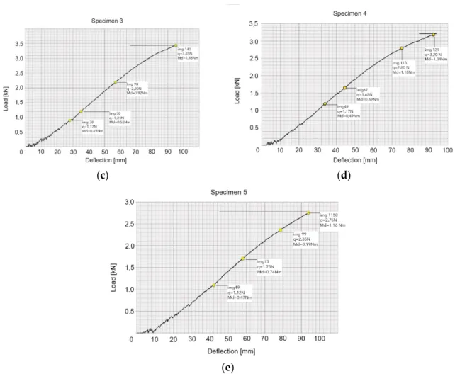
(e)
Figure 8. Load-deflection diagrams obtained in the test: (a) Specimen 1; (b) Specimen 2; (c) Specimen 3; (d) Specimen 4; and (e) Specimen 5.
5. Parameters of the Analysis
It is important to identify those significant parameters which are worth being analyzed to detect and quantify cracks. Firstly, a selection of geometrical parameters to consider during the image post-processing for crack detection is needed. Secondly, a selection of significant parameters to consider is also required to quantify the phenomenon of cracking and the loading status of the beam.
5.1. Parameters to Use in the Processing Process for Crack Detection
Color and geometrical parameters were considered in the first steps of image post-processing, only oriented to identify the cracks and by following the existing literature about image processing about cracking of concrete, e.g., work done by Astushi et al. [19], Otsu [20], Gonzalez et al. [21] and Yamaguchi et al. [22]. These parameters are based on the fact of having all images at the same scale and converted into grey scale to make the selection easier.
5.1.1. Saturation of Color
The saturation of black color in some areas reveals the appearance of a crack and this provides the first selection among the existing shadows; different values such as the mean grey, the standard deviation, the modal grey, the minimum and maximum grey levels and the integrated density may be evaluated more specifically to detect the cracks.
5.1.2. Geometry
Geometry of a crack may be basically defined by the area, the circularity and solidity. Figure 8.Load-deflection diagrams obtained in the test: (a) Specimen 1; (b) Specimen 2; (c) Specimen 3; (d) Specimen 4; and (e) Specimen 5.
5. Parameters of the Analysis
It is important to identify those significant parameters which are worth being analyzed to detect and quantify cracks. Firstly, a selection of geometrical parameters to consider during the image post-processing for crack detection is needed. Secondly, a selection of significant parameters to consider is also required to quantify the phenomenon of cracking and the loading status of the beam. 5.1. Parameters to Use in the Processing Process for Crack Detection
Color and geometrical parameters were considered in the first steps of image post-processing, only oriented to identify the cracks and by following the existing literature about image processing about cracking of concrete, e.g., work done by Astushi et al. [19], Otsu [20], Gonzalez et al. [21] and Yamaguchi et al. [22]. These parameters are based on the fact of having all images at the same scale and converted into grey scale to make the selection easier.
5.1.1. Saturation of Color
The saturation of black color in some areas reveals the appearance of a crack and this provides the first selection among the existing shadows; different values such as the mean grey, the standard deviation, the modal grey, the minimum and maximum grey levels and the integrated density may be evaluated more specifically to detect the cracks.
Buildings2018,8, 158 10 of 21
5.1.2. Geometry
Geometry of a crack may be basically defined by the area, the circularity and solidity.
The area of a crack is defined thanks to the segment detection option (available in most software) by using selective saturation of black in the grey scale. The definition of a specific area for a crack depends on the limit which is specified in saturation options.
Circularity refers to the similarity to a circle of defined segments. It is interesting to separate regular cracks from small holes and others, and the expression which may define it is Equation (4), ranging from 0 to 1, being 0 very similar to a circle and 1 very similar to a linear element. This way, interferences may be detected when circularity is far from 1. Most image post-processing software allows quantifying circularity when detecting specific segments.
C=4·π·(Area)/
Perimeter2 (4)
Solidity determines the ratio between area and perimeter of a specific segment (or crack). The formula to quantify solidity is mentioned below, being “Convex Area” the one which is contained by a convex polyline without inner interferences.
S= (Area)/(Convex Area) (5)
5.2. Parameters to Use in the Analysis for Crack Quantification
Once cracks have been faithfully identified through initial color and geometrical parameters, the second step is to quantify their magnitude to determine structural behaviors. For this purpose, three significant parameters have been identified: the crack opening width, the growth pattern and the crack spacing distance.
5.2.1. Crack Opening Width
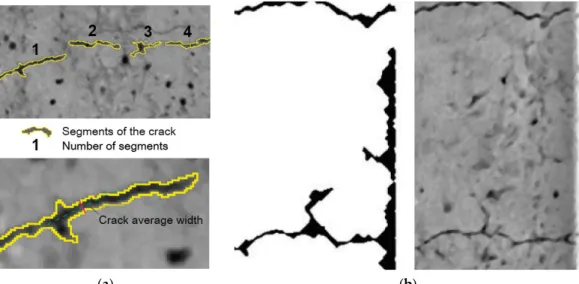
The crack opening width is the most important parameter to quantify cracking of a concrete element and, therefore, the loading status. Eurocode 2 [14] and Spanish Standard EHE-08 [15] base the cracking control in RC elements by the crack opening width limitation. However, those measured cracks from shots are not always continuous (see Figure9a); thus, different segments must be previously detected separately and width must be obtained as a mean value. Voids in RC elements are usually derived from the process of concreting. During the segment detection, voids may lead to confusion and this should be avoided thanks to the evaluation of circularity (see Figure10).
Buildings 2018, 8, x FOR PEER REVIEW 10 of 21
The area of a crack is defined thanks to the segment detection option (available in most software) by using selective saturation of black in the grey scale. The definition of a specific area for a crack depends on the limit which is specified in saturation options.
Circularity refers to the similarity to a circle of defined segments. It is interesting to separate regular cracks from small holes and others, and the expression which may define it is Equation (4), ranging from 0 to 1, being 0 very similar to a circle and 1 very similar to a linear element. This way, interferences may be detected when circularity is far from 1. Most image post-processing software allows quantifying circularity when detecting specific segments.
𝐶 = 4 · 𝜋 · (𝐴𝑟𝑒𝑎)/(𝑃𝑒𝑟𝑖𝑚𝑒𝑡𝑒𝑟 ) (4)
Solidity determines the ratio between area and perimeter of a specific segment (or crack). The formula to quantify solidity is mentioned below, being “Convex Area” the one which is contained by a convex polyline without inner interferences.
𝑆 = (𝐴𝑟𝑒𝑎)/(𝐶𝑜𝑛𝑣𝑒𝑥 𝐴𝑟𝑒𝑎) (5)
5.2. Parameters to Use in the Analysis for Crack Quantification
Once cracks have been faithfully identified through initial color and geometrical parameters, the second step is to quantify their magnitude to determine structural behaviors. For this purpose, three significant parameters have been identified: the crack opening width, the growth pattern and the crack spacing distance.
5.2.1. Crack Opening Width
The crack opening width is the most important parameter to quantify cracking of a concrete element and, therefore, the loading status. Eurocode 2 [14] and Spanish Standard EHE-08 [15] base the cracking control in RC elements by the crack opening width limitation. However, those measured cracks from shots are not always continuous (see Figure 9a); thus, different segments must be previously detected separately and width must be obtained as a mean value. Voids in RC elements are usually derived from the process of concreting. During the segment detection, voids may lead to confusion and this should be avoided thanks to the evaluation of circularity (see Figure 10).
(a) (b)
Figure 9. Measurement and detection of cracks: (a) measurement of crack opening width as a mean value; and (b) “boundary effect” in segment detection.
Figure 9.Measurement and detection of cracks: (a) measurement of crack opening width as a mean value; and (b) “boundary effect” in segment detection.
Buildings2018,8, 158 11 of 21
Buildings 2018, 8, x FOR PEER REVIEW 11 of 21
Figure 10. Crack opening width must be obtained from a mean value, due to the interference of voids. 5.2.2. Growth Pattern
The patterns of growth of structural cracks mainly responds to the typology and levels of loading. Although the evolution of the loading status of a joist is not only related to the increment of the crack opening width, it is a significant parameter to consider to quantify the loading status. As explained above, the crack opening width in RC elements must be quantified as a mean value of several measurements due to the irregularity of the perimeter. Width of cracks under pure bending grows until the collapse. For instance, the crack opening width in Specimen 1 under 270 kg of load is two times the width under 135 kg.
Since cracking starts from the perimeter of the concrete section, with usually lower reinforcement ratios, a “boundary effect” may occur (see Figure 9b); detected segments starting at the boundary may generate confusion with cracks itself; thus, it is highly recommended to crop the image of the beam just to avoid this phenomenon.
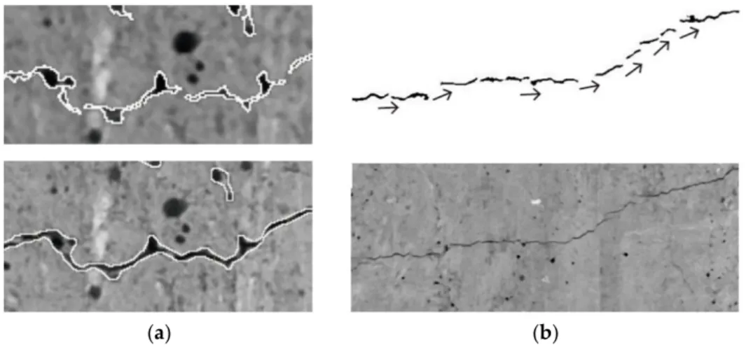
Besides, cracks are often not continuous, although the continuity grows hand in hand with load. Discontinuous segments have to be detected by image post-processing to draw the full path of the crack, which may tell a lot about their origin and nature (see Figure 11).
(a) (b)
Figure 11. Growth pattern of cracks detection: (a) proximity between segments of a crack reveals its growth pattern; and (b) final path of the measured crack tells about the loading pattern.
5.2.3. Crack Spacing
Crack spacing is the third decisive parameter, together with the opening width, that clearly allows defining the cracking and loading status of the beam. Crack spacing has to be measured as a mean value of several measurements due to the inherent irregularity of the material (Figure 12), but at the same time it reveals important information about the loading pattern, as well as the geometry and location of reinforcements. The spacing between cracks is usually the same from the first instant of loading, thus the diameter and spacing of reinforcement bars are crucial issues.
Figure 10.Crack opening width must be obtained from a mean value, due to the interference of voids. 5.2.2. Growth Pattern
The patterns of growth of structural cracks mainly responds to the typology and levels of loading. Although the evolution of the loading status of a joist is not only related to the increment of the crack opening width, it is a significant parameter to consider to quantify the loading status. As explained above, the crack opening width in RC elements must be quantified as a mean value of several measurements due to the irregularity of the perimeter. Width of cracks under pure bending grows until the collapse. For instance, the crack opening width in Specimen 1 under 270 kg of load is two times the width under 135 kg.
Since cracking starts from the perimeter of the concrete section, with usually lower reinforcement ratios, a “boundary effect” may occur (see Figure9b); detected segments starting at the boundary may generate confusion with cracks itself; thus, it is highly recommended to crop the image of the beam just to avoid this phenomenon.
Besides, cracks are often not continuous, although the continuity grows hand in hand with load. Discontinuous segments have to be detected by image post-processing to draw the full path of the crack, which may tell a lot about their origin and nature (see Figure11).
Buildings 2018, 8, x FOR PEER REVIEW 11 of 21
Figure 10. Crack opening width must be obtained from a mean value, due to the interference of voids. 5.2.2. Growth Pattern
The patterns of growth of structural cracks mainly responds to the typology and levels of loading. Although the evolution of the loading status of a joist is not only related to the increment of the crack opening width, it is a significant parameter to consider to quantify the loading status. As explained above, the crack opening width in RC elements must be quantified as a mean value of several measurements due to the irregularity of the perimeter. Width of cracks under pure bending grows until the collapse. For instance, the crack opening width in Specimen 1 under 270 kg of load is two times the width under 135 kg.
Since cracking starts from the perimeter of the concrete section, with usually lower reinforcement ratios, a “boundary effect” may occur (see Figure 9b); detected segments starting at the boundary may generate confusion with cracks itself; thus, it is highly recommended to crop the image of the beam just to avoid this phenomenon.
Besides, cracks are often not continuous, although the continuity grows hand in hand with load. Discontinuous segments have to be detected by image post-processing to draw the full path of the crack, which may tell a lot about their origin and nature (see Figure 11).
(a) (b)
Figure 11. Growth pattern of cracks detection: (a) proximity between segments of a crack reveals its growth pattern; and (b) final path of the measured crack tells about the loading pattern.
5.2.3. Crack Spacing
Crack spacing is the third decisive parameter, together with the opening width, that clearly allows defining the cracking and loading status of the beam. Crack spacing has to be measured as a mean value of several measurements due to the inherent irregularity of the material (Figure 12), but at the same time it reveals important information about the loading pattern, as well as the geometry and location of reinforcements. The spacing between cracks is usually the same from the first instant of loading, thus the diameter and spacing of reinforcement bars are crucial issues.
Figure 11.Growth pattern of cracks detection: (a) proximity between segments of a crack reveals its growth pattern; and (b) final path of the measured crack tells about the loading pattern.
5.2.3. Crack Spacing
Crack spacing is the third decisive parameter, together with the opening width, that clearly allows defining the cracking and loading status of the beam. Crack spacing has to be measured as a mean value of several measurements due to the inherent irregularity of the material (Figure12), but at the same time it reveals important information about the loading pattern, as well as the geometry and location of reinforcements. The spacing between cracks is usually the same from the first instant of loading, thus the diameter and spacing of reinforcement bars are crucial issues.
Buildings2018,8, 158 12 of 21
Buildings 2018, 8, x FOR PEER REVIEW 12 of 21
Figure 12. Measurement of crack spacing distance as a mean value in projection. 6. Image Post-Processing Analysis Method
The obtained shots allow drawing a progressive time-lapse of generated cracks in all five specimens. These sequences of high-res images provide huge amounts of information to be analyzed; however, this analysis is not free from a couple of challenges that must be faced. Firstly, it should be considered that specimens deflect significantly while the camera is fixed below; this means that the distance between the cracks and the lens vary from the beginning to the end, a fact that requires updating the scale at each loading stage. Secondly, marks and shadows were detected on the concrete surface of specimens, which means that complex post-processing must be done to classify them apart from cracks (Figure 13).
Figure 13. Detected marks and shadows on concrete surface.
To carry out the required image post-processing, preliminary image enhancements were needed to prepare the shots, followed by the post-processing itself. The entire process was done using Photoshop CC 2017 and ImageJ software.
6.1. Image Pre-Processing
6.1.1. Correction of Optical Aberrations
It consists in correcting the existing aberrations, such as the slight optical curvature caused by the geometry of lens itself. This was done using the “Straighten” and “Remove Distortion” tools. The former was used to align the specimens with the image framework in case of showing deviations to crop it more easily (Figure 14a,b). The latter was used to correct the slight curvature of specimens caused by the lens to work on similar flat images; this tool was calibrated using a superimposed grid which allows fitting linear shapes.
Figure 12.Measurement of crack spacing distance as a mean value in projection. 6. Image Post-Processing Analysis Method
The obtained shots allow drawing a progressive time-lapse of generated cracks in all five specimens. These sequences of high-res images provide huge amounts of information to be analyzed; however, this analysis is not free from a couple of challenges that must be faced. Firstly, it should be considered that specimens deflect significantly while the camera is fixed below; this means that the distance between the cracks and the lens vary from the beginning to the end, a fact that requires updating the scale at each loading stage. Secondly, marks and shadows were detected on the concrete surface of specimens, which means that complex post-processing must be done to classify them apart from cracks (Figure13).
Buildings 2018, 8, x FOR PEER REVIEW 12 of 21
Figure 12. Measurement of crack spacing distance as a mean value in projection. 6. Image Post-Processing Analysis Method
The obtained shots allow drawing a progressive time-lapse of generated cracks in all five specimens. These sequences of high-res images provide huge amounts of information to be analyzed; however, this analysis is not free from a couple of challenges that must be faced. Firstly, it should be considered that specimens deflect significantly while the camera is fixed below; this means that the distance between the cracks and the lens vary from the beginning to the end, a fact that requires updating the scale at each loading stage. Secondly, marks and shadows were detected on the concrete surface of specimens, which means that complex post-processing must be done to classify them apart from cracks (Figure 13).
Figure 13. Detected marks and shadows on concrete surface.
To carry out the required image post-processing, preliminary image enhancements were needed to prepare the shots, followed by the post-processing itself. The entire process was done using Photoshop CC 2017 and ImageJ software.
6.1. Image Pre-Processing
6.1.1. Correction of Optical Aberrations
It consists in correcting the existing aberrations, such as the slight optical curvature caused by the geometry of lens itself. This was done using the “Straighten” and “Remove Distortion” tools. The former was used to align the specimens with the image framework in case of showing deviations to crop it more easily (Figure 14a,b). The latter was used to correct the slight curvature of specimens caused by the lens to work on similar flat images; this tool was calibrated using a superimposed grid which allows fitting linear shapes.
Figure 13.Detected marks and shadows on concrete surface.
To carry out the required image post-processing, preliminary image enhancements were needed to prepare the shots, followed by the post-processing itself. The entire process was done using Photoshop CC 2017 and ImageJ software.
6.1. Image Pre-Processing
6.1.1. Correction of Optical Aberrations
It consists in correcting the existing aberrations, such as the slight optical curvature caused by the geometry of lens itself. This was done using the “Straighten” and “Remove Distortion” tools. The former was used to align the specimens with the image framework in case of showing deviations to crop it more easily (Figure14a,b). The latter was used to correct the slight curvature of specimens caused by the lens to work on similar flat images; this tool was calibrated using a superimposed grid which allows fitting linear shapes.
Buildings2018,8, 158 13 of 21
Buildings 2018, 8, x FOR PEER REVIEW 13 of 21
(a) (b)
Figure 14. First enhancements: (a) original image; and (b) image without optical aberrations. 6.1.2. Identification of Specimens
The second preliminary enhancement was to detect specimens in the shot and to crop them to have the same width in pixels in all images. In this case, a value of 1023 pixels has been fixed for the length.
6.1.3. Correction of Brightness
The third adjustment consists in correcting brightness so that the histogram curve of the image becomes in the center; this way, different images of the same element have the same level of brightness. This is important when being analyzed to choose the same value of threshold.
6.1.4. Reduction of Marks
The specimens were affected by some blue marks and other shadows on the surface of concrete (see Figure 15) due to irregularities of the concrete itself. Thus, the fourth adjustment consisted in reducing these existing perturbations. The image was converted into greyscale, thus it becomes possible to easily eliminate desired areas from the binary image.
The conversion into a grayscale image was done by using the automatic option; this provides better results than doing it manually canal by canal. This works well to eliminate the existing blue stains but certain information about the cracks is lost.
(a) (b)
Figure 14.First enhancements: (a) original image; and (b) image without optical aberrations. 6.1.2. Identification of Specimens
The second preliminary enhancement was to detect specimens in the shot and to crop them to have the same width in pixels in all images. In this case, a value of 1023 pixels has been fixed for the length.
6.1.3. Correction of Brightness
The third adjustment consists in correcting brightness so that the histogram curve of the image becomes in the center; this way, different images of the same element have the same level of brightness. This is important when being analyzed to choose the same value of threshold.
6.1.4. Reduction of Marks
The specimens were affected by some blue marks and other shadows on the surface of concrete (see Figure15) due to irregularities of the concrete itself. Thus, the fourth adjustment consisted in reducing these existing perturbations. The image was converted into greyscale, thus it becomes possible to easily eliminate desired areas from the binary image.
Buildings 2018, 8, x FOR PEER REVIEW 13 of 21
(a) (b)
Figure 14. First enhancements: (a) original image; and (b) image without optical aberrations. 6.1.2. Identification of Specimens
The second preliminary enhancement was to detect specimens in the shot and to crop them to have the same width in pixels in all images. In this case, a value of 1023 pixels has been fixed for the length.
6.1.3. Correction of Brightness
The third adjustment consists in correcting brightness so that the histogram curve of the image becomes in the center; this way, different images of the same element have the same level of brightness. This is important when being analyzed to choose the same value of threshold.
6.1.4. Reduction of Marks
The specimens were affected by some blue marks and other shadows on the surface of concrete (see Figure 15) due to irregularities of the concrete itself. Thus, the fourth adjustment consisted in reducing these existing perturbations. The image was converted into greyscale, thus it becomes possible to easily eliminate desired areas from the binary image.
The conversion into a grayscale image was done by using the automatic option; this provides better results than doing it manually canal by canal. This works well to eliminate the existing blue stains but certain information about the cracks is lost.
(a) (b)
Figure 15. First enhancements: (a) correction of brightness: centered histogram; and (b) reduction of dust.
Buildings2018,8, 158 14 of 21
The conversion into a grayscale image was done by using the automatic option; this provides better results than doing it manually canal by canal. This works well to eliminate the existing blue stains but certain information about the cracks is lost.
6.1.5. Variation of Color Levels
Ultimately, color levels were varied to extend the spectrum of grey levels, maximizing the information in the images. Final obtained images are much clearer to obtain information (Figure16).
Buildings 2018, 8, x FOR PEER REVIEW 14 of 21
Figure 15. First enhancements: (a) correction of brightness: centered histogram; and (b) reduction of dust.
6.1.5. Variation of Color Levels
Ultimately, color levels were varied to extend the spectrum of grey levels, maximizing the information in the images. Final obtained images are much clearer to obtain information (Figure 16).
Figure 16. Original and pre-processed image after initial enhancements. 6.2. Image Post-Processing
6.2.1. Binary Conversion and Threshold
The pre-processed image is reduced into black and white in this step. In the process of conversion into binary scale of color, it is necessary to establish specific values for the threshold to maximize the information of the shot, according to Atsushi et al. [19]. These authors proposed a value “k” for the threshold, after calibration of several experimental tests, with the following value:
k = average gray + min/1.25 (4)
where average grey is the brightness average in the whole area and min is the minimum of brightness in the whole area.
In this case, a value of k = 118 with a percentage of 5.02% was considered (see Figure 17); by assuming the “Intermodes” option, a bimodal histogram was chosen. The histogram then had to be softened iteratively using an average size of 3 pixel, by moving between two local maximum values “j” and “k”. Then, the threshold value “T” was calculated as (j + k)/2. This value allowed including the majority of cracks while keeping some significant stains (Figure 17), which were reduced in the next steps.
Figure 17. Shot after binary conversion and thresholding. 6.2.2. Scale and Size Adjustments
At this phase, it is important to set the scale of the shot by knowing that the real width of the beam is 125 mm. Knowing that the shot is 1024 pixel wide, 8.2 pixels correspond to 1 mm, i.e., each
Figure 16.Original and pre-processed image after initial enhancements. 6.2. Image Post-Processing
6.2.1. Binary Conversion and Threshold
The pre-processed image is reduced into black and white in this step. In the process of conversion into binary scale of color, it is necessary to establish specific values for the threshold to maximize the information of the shot, according to Atsushi et al. [19]. These authors proposed a value “k” for the threshold, after calibration of several experimental tests, with the following value:
k = average gray + min/1.25 (4)
where average grey is the brightness average in the whole area and min is the minimum of brightness in the whole area.
In this case, a value of k = 118 with a percentage of 5.02% was considered (see Figure 17); by assuming the “Intermodes” option, a bimodal histogram was chosen. The histogram then had to be softened iteratively using an average size of 3 pixel, by moving between two local maximum values “j” and “k”. Then, the threshold value “T” was calculated as (j + k)/2. This value allowed including the majority of cracks while keeping some significant stains (Figure17), which were reduced in the next steps.
Buildings 2018, 8, x FOR PEER REVIEW 14 of 21
Figure 15. First enhancements: (a) correction of brightness: centered histogram; and (b) reduction of dust.
6.1.5. Variation of Color Levels
Ultimately, color levels were varied to extend the spectrum of grey levels, maximizing the information in the images. Final obtained images are much clearer to obtain information (Figure 16).
Figure 16. Original and pre-processed image after initial enhancements. 6.2. Image Post-Processing
6.2.1. Binary Conversion and Threshold
The pre-processed image is reduced into black and white in this step. In the process of conversion into binary scale of color, it is necessary to establish specific values for the threshold to maximize the information of the shot, according to Atsushi et al. [19]. These authors proposed a value “k” for the threshold, after calibration of several experimental tests, with the following value:
k = average gray + min/1.25 (4)
where average grey is the brightness average in the whole area and min is the minimum of brightness in the whole area.
In this case, a value of k = 118 with a percentage of 5.02% was considered (see Figure 17); by assuming the “Intermodes” option, a bimodal histogram was chosen. The histogram then had to be softened iteratively using an average size of 3 pixel, by moving between two local maximum values “j” and “k”. Then, the threshold value “T” was calculated as (j + k)/2. This value allowed including the majority of cracks while keeping some significant stains (Figure 17), which were reduced in the next steps.
Figure 17. Shot after binary conversion and thresholding. 6.2.2. Scale and Size Adjustments
At this phase, it is important to set the scale of the shot by knowing that the real width of the beam is 125 mm. Knowing that the shot is 1024 pixel wide, 8.2 pixels correspond to 1 mm, i.e., each
Buildings2018,8, 158 15 of 21
6.2.2. Scale and Size Adjustments
At this phase, it is important to set the scale of the shot by knowing that the real width of the beam is 125 mm. Knowing that the shot is 1024 pixel wide, 8.2 pixels correspond to 1 mm, i.e., each pixel represents an area of 0.12 mm×0.12 mm of the joist. By considering the standard limits for width cracks of 0.2 mm, the maximum opening width should correspond to 2 pixels.
6.2.3. Filtering of Particles
Shots with the binary conversion and faithfully scaled still show a lot of noise in terms of particles out of the cracks themselves. By using the “Analyze Particles” tool available in ImageJ software and others, it is possible to choose the particles to filter (Figure18a); the goal is to create a mask by filtering segments by area and circularity to isolate cracks. The difficulty lies in detecting the right segment corresponding with cracks; thus, a test to analyze proportions of existing cracks to obtain the limit values to introduce into the chart was needed. Regarding circularity, a limit value of 50% was chosen to eliminate depressions and voids that are more similar to a circle.
Buildings 2018, 8, x FOR PEER REVIEW 15 of 21
pixel represents an area of 0.12 mm × 0.12 mm of the joist. By considering the standard limits for width cracks of 0.2 mm, the maximum opening width should correspond to 2 pixels.
6.2.3. Filtering of Particles
Shots with the binary conversion and faithfully scaled still show a lot of noise in terms of particles out of the cracks themselves. By using the “Analyze Particles” tool available in ImageJ software and others, it is possible to choose the particles to filter (Figure 18a); the goal is to create a mask by filtering segments by area and circularity to isolate cracks. The difficulty lies in detecting the right segment corresponding with cracks; thus, a test to analyze proportions of existing cracks to obtain the limit values to introduce into the chart was needed. Regarding circularity, a limit value of 50% was chosen to eliminate depressions and voids that are more similar to a circle.
(a) (b)
Figure 18. Image post-processing: (a) “Analyze Particles” tool: circularity; and (b) joining of discontinuous segments by using binary options.
6.2.4. Joining of Discontinuous Segments
Detected cracks show discontinuities at some points, which imply some difficulties in identifying their origin. These segments can be easily completed by using morphologic operations; optimum interrelations can be found to link isolated parts without distorting the width or the shape of the crack (Figure 18b).
6.2.5. Superimposing Masks and Final Evaluation
It is interesting to superimpose masks of “particle analysis” and “close segments” with the original image to determine which is more convenient. After all image post-processing, it was necessary to determine the best procedure to ensure a faithful quantification of cracks.
6.3. Outline of the Image Post-Processing Method for Crack Quantification
The proposed image-based processing method is outlined in Figure 19, from the original shot to the final image that allows quantifying the mechanical features of the cracks.
Figure 18.Image post-processing: (a) “Analyze Particles” tool: circularity; and (b) joining of discontinuous segments by using binary options.
6.2.4. Joining of Discontinuous Segments
Detected cracks show discontinuities at some points, which imply some difficulties in identifying their origin. These segments can be easily completed by using morphologic operations; optimum interrelations can be found to link isolated parts without distorting the width or the shape of the crack (Figure18b).
6.2.5. Superimposing Masks and Final Evaluation
It is interesting to superimpose masks of “particle analysis” and “close segments” with the original image to determine which is more convenient. After all image post-processing, it was necessary to determine the best procedure to ensure a faithful quantification of cracks.
Buildings2018,8, 158 16 of 21
6.3. Outline of the Image Post-Processing Method for Crack Quantification
The proposed image-based processing method is outlined in Figure19, from the original shot to the final image that allows quantifying the mechanical features of the cracks.Buildings 2018, 8, x FOR PEER REVIEW 16 of 21
Figure 19. Proposed image-based processing method. 7. Evaluation of the Image Post-Processing Method
To evaluate the proposed image post-processing method for crack quantification in RC elements under bending, this study compared the values of crack opening widths and spacing obtained from shot measurements with those predicted by the standards. By using the results of the experimental campaign described in Section 4, the features of measured cracks (opening width and spacing) in shots were compared with those calculated by using the Eurocode approach.
7.1. Limits and Points of Measurement
The suggested serviceability limit for crack opening width in reinforced concrete elements is 0.20 mm [15,16]. Assuming that this is the first value which may be faithfully detected by using image post-processing, this study starts evaluating the method at this stage.
Between the SLS cracking limit of 0.2 mm and the maximum measured value of opening crack width, two more intermediate points were chosen for analysis. Knowing all geometrical and material properties of RC joists, it is possible to link the crack opening width and spacing with deflection, the acting bending moment and even the loading status. Classical theory and the standards about cracking phenomenon in RC elements define different approaches to determine these values under specific loading states.
To faithfully evaluate the method, the crack measurement from shots was done at five different points per crack; by assuming a number between 10 and 12 cracks per specimen in central length, this measurement leads to 50 measurements per analyzed shot. Under pure bending, the opening of all cracks keeps very similar thanks to the assumption of constant curvature.
7.2. Comparison between Measured and Predicted Values
Four different shots per specimen were used (the test included up to one shot per 2.5 kg of load increment); these selected shots belong to four different loading stages, corresponding to the points in Figure 20. Two significant parameters were considered to evaluate the proposed method: the mean
Figure 19.Proposed image-based processing method. 7. Evaluation of the Image Post-Processing Method
To evaluate the proposed image post-processing method for crack quantification in RC elements under bending, this study compared the values of crack opening widths and spacing obtained from shot measurements with those predicted by the standards. By using the results of the experimental campaign described in Section4, the features of measured cracks (opening width and spacing) in shots were compared with those calculated by using the Eurocode approach.
7.1. Limits and Points of Measurement
The suggested serviceability limit for crack opening width in reinforced concrete elements is 0.20 mm [15,16]. Assuming that this is the first value which may be faithfully detected by using image post-processing, this study starts evaluating the method at this stage.
Between the SLS cracking limit of 0.2 mm and the maximum measured value of opening crack width, two more intermediate points were chosen for analysis. Knowing all geometrical and material properties of RC joists, it is possible to link the crack opening width and spacing with deflection, the acting bending moment and even the loading status. Classical theory and the standards about cracking phenomenon in RC elements define different approaches to determine these values under specific loading states.
To faithfully evaluate the method, the crack measurement from shots was done at five different points per crack; by assuming a number between 10 and 12 cracks per specimen in central length, this measurement leads to 50 measurements per analyzed shot. Under pure bending, the opening of all cracks keeps very similar thanks to the assumption of constant curvature.
Buildings2018,8, 158 17 of 21
7.2. Comparison between Measured and Predicted Values
Four different shots per specimen were used (the test included up to one shot per 2.5 kg of load increment); these selected shots belong to four different loading stages, corresponding to the points in Figure20. Two significant parameters were considered to evaluate the proposed method: the mean crack opening width and the mean crack spacing. In Tables1–5, measured and predicted values for both parameters are shown; a good accuracy between measured and theoretical values is observed, provided that cracking of concrete becomes sometimes difficult to predict.
Table 1.Measured and calculated results for Specimen 1.
Image Av. Min. k
Crack Width Image Crack Width Analysis Sm Image Sm Analysis Ferret Av. Crack Area Crack Area Image 64 142 0 113.6 0.32 0.15 58.00 63.79 470.82 150.66 399.54 78 148 0 118.4 0.35 0.23 61.10 63.79 549.42 175.81 389.02 90 146 0 116.8 0.41 0.32 58.80 63.79 932.08 326.23 863.98 131 153 0 122.4 0.62 0.58 58.58 63.79 1142.75 708.50 1316.86 Measurements in mm.
Table 2.Measured and calculated results for Specimen 2.
Image Av. Min. k
Crack Width Image Crack Width Analysis Sm Image Sm Analysis Ferret Av. Crack Area Crack Area Image 54 142 0 113.6 0.32 0.20 57.41 57.12 474.20 151.74 418.46 74 154 0 123.8 0.35 0.27 52.33 57.12 701.26 245.44 454.86 88 140 0 112.5 0.38 0.32 48.59 57.12 1083.71 411.81 708.21 101 148 0 118.6 0.45 0.36 42.88 57.12 1208.94 544.02 1087.54 Measurements in mm.
Table 3.Measured and calculated results for Specimen 3.
Image Av. Min. k
Crack Width Image Crack Width Analysis Sm Image Sm Analysis Ferret Av. Crack Area Crack Area Image 38 135 0 108.0 0.29 0.19 60.31 61.92 76.42 22.16 43.38 49 137 0 109.6 0.30 0.20 60.39 61.92 318.24 95.47 259.04 90 131 0 104.8 0.41 0.35 63.12 61.92 685.92 281.23 599.90 140 133 0 106.4 0.58 0.56 54.56 61.92 962.50 558.25 1023.54 Measurements in mm.
Table 4.Measured and calculated results for Specimen 4.
Image Av. Min. k
Crack Width Image Crack Width Analysis Sm Image Sm Analysis Ferret Av. Crack Area Crack Area Image 49 158 0 126.4 0.23 0.20 65.40 53.15 109.88 25.27 98.28 68 142 0 113.6 0.29 0.29 68.43 53.15 420.61 121.98 322.46 113 138 0 110.4 0.50 0.50 58.75 53.15 779.75 389.88 1027.58 129 139 0 111.2 0.59 0.56 60.41 53.15 779.40 459.85 1111.73 Measurements in mm.
Regarding the crack opening width, although having a notorious scatter of results due to the inherent uncertainty of the phenomenon, the mean of measured and predicted values tend to match quite accurately as cracks get wider. At first stages of cracking, the difference between the values is clearly significant (up to 0.17 mm) due to the hazardous generation of early cracks. In Figure20, mean values of measured and calculated crack opening width are shown.
![Figure 1. Reinforced RC joists (without pre-stressing) are commonly used in northern Spain areas: (a) lateral view of typical RC joists; and (b) general view of the one-way ribbed slabs, source: Iberaceros Forjados Riojanos, [4]](https://thumb-us.123doks.com/thumbv2/123dok_us/1866318.2772128/2.892.127.768.376.630/figure-reinforced-stressing-commonly-northern-iberaceros-forjados-riojanos.webp)
![Figure 2. Uniaxial stress-strain curve for plain concrete. Source: [14].](https://thumb-us.123doks.com/thumbv2/123dok_us/1866318.2772128/3.892.285.607.300.581/figure-uniaxial-stress-strain-curve-plain-concrete-source.webp)
![Figure 4. Effective height, h c,eff according to Eurocode 2 [13].](https://thumb-us.123doks.com/thumbv2/123dok_us/1866318.2772128/5.892.303.593.277.423/figure-effective-height-according-eurocode-centroid-effective-tensioned.webp)