Linear Models and Empirical Bayes Methods for
Assessing Differential Expression in Microarray
Experiments
∗
Gordon K. Smyth
Walter and Eliza Hall Institute of Medical Research
Melbourne, Vic 3050, Australia
January 2004
†Abstract
The problem of identifying differentially expressed genes in designed microar-ray experiments is considered. L¨onnstedt and Speed (2002) derived an expression for the posterior odds of differential expression in a replicated two-color experi-ment using a simple hierarchical parametric model. The purpose of this paper is to develop the hierarchical model of L¨onnstedt and Speed (2002) into a practical approach for general microarray experiments with arbitrary numbers of treat-ments and RNA samples. The model is reset in the context of general linear models with arbitrary coefficients and contrasts of interest. The approach applies equally well to both single channel and two color microarray experiments. Con-sistent, closed form estimators are derived for the hyperparameters in the model. The estimators proposed have robust behavior even for small numbers of arrays and allow for incomplete data arising from spot filtering or spot quality weights. The posterior odds statistic is reformulated in terms of a moderated t-statistic in which posterior residual standard deviations are used in place of ordinary stan-dard deviations. The empirical Bayes approach is equivalent to shrinkage of the estimated sample variances towards a pooled estimate, resulting in far more stable inference when the number of arrays is small. The use of moderated t-statistics has the advantage over the posterior odds that the number of hyperparameters which need to estimated is reduced; in particular, knowledge of the non-null prior for the fold changes are not required. The moderated t-statistic is shown to follow a t-distribution with augmented degrees of freedom. The moderated t inferential approach extends to accommodate tests of composite null hypotheses through the ∗Please cite as: Smyth, G. K. (2004). Linear models and empirical Bayes methods for assessing
differential expression in microarray experiments. Statistical Applications in Genetics and Molecular BiologyVolume 3, Issue 1, Article 3.
use of moderated F-statistics. The performance of the methods is demonstrated in a simulation study. Results are presented for two publicly available data sets.
Keywords: microarrays, empirical Bayes, linear models, hyperparameters, dif-ferential expression
1
Introduction
Microarrays are a technology for comparing the expression profiles of genes on a genomic scale across two or more RNA samples. Recent reviews of microarray data analysis include the Nature Genetics supplement (2003), Smyth et al (2003), Parmigiani et al (2003) and Speed (2003). This paper considers the problem of identifying genes which are differentially expressed across specified conditions in designed microarray experiments. This is a massive multiple testing problem in which one or more tests are conducted for each of tens of thousands of genes. The problem is complicated by the fact that the measured expression levels are often non-normally distributed and have non-identical and dependent distributions between genes. This paper addresses particularly the fact that the variability of the expression values differs between genes. It is well established that allowance needs to be made in the analysis of microarray experiments for the amount of multiple testing, perhaps by controlling the familywise error rate or the false discovery rate, even though this reduces the power available to detect changes in expression for individual genes (Ge et al, 2002). On the other hand, the parallel nature of the inference in microarrays allows some compensating possibilities for borrowing information from the ensemble of genes which can assist in inference about each gene individually. One way that this can be done is through the application of Bayes or empirical Bayes methods (Efron, 2001, 2003). Efron et al (2001) used a non-parametric empirical Bayes approach for the analysis of factorial data with high density oligonucleotide microarray data. This approach has much potential but can be difficult to apply in practical situations especially by less experienced practitioners. L¨onnstedt and Speed (2002), considering replicated two-color microarray experiments, took instead a parametric empirical Bayes approach using a simple mixture of normal models and a conjugate prior and derived a pleasingly simple expression for the posterior odds of differential expression for each gene. The posterior odds expression has proved to be a useful means of ranking genes in terms of evidence for differential expression.
The purpose of this paper is to develop the hierarchical model of L¨onnstedt and Speed (2002) into a practical approach for general microarray experiments with arbi-trary numbers of treatments and RNA samples. The first step is to reset it in the context of general linear models with arbitrary coefficients and contrasts of interest. The approach applies to both single channel and two color microarrays. All of the commonly used microarray platforms such as cDNA, long-oligos and Affymetrix are therefore accommodated. The second step is to derive consistent, closed form estima-tors for the hyperparameters using the marginal distributions of the observed statistics. The estimators proposed here have robust behavior even for small numbers of arrays and allow for incomplete data arising from spot filtering or spot quality weights. The third
step is to reformulate the posterior odds statistic in terms of a moderated t-statistic in which posterior residual standard deviations are used in place of ordinary standard deviations. This approach makes explicit what was implicit in L¨onnstedt and Speed (2002), that the hierarchical model results in a shrinkage of the gene-wise residual sam-ple variances towards a common value, resulting in far more stable inference when the number of arrays is small. The use of moderated t-statistic has the advantage over the posterior odds of reducing the number of hyperparameters which need to estimated under the hierarchical model; in particular, knowledge of the non-null prior for the fold changes are not required. The moderated t-statistic is shown to follow a t-distribution with augmented degrees of freedom. The moderated t inferential approach extends to accommodate tests involving two or more contrasts through the use of moderated
F-statistics.
The idea of using a t-statistic with a Bayesian adjusted denominator was also pro-posed by Baldi and Long (2001) who developed the useful cyberT program. Their work was limited though to two-sample control versus treatment designs and their model did not distinguish between differentially and non-differentially expressed genes. They also did not develop consistent estimators for the hyperparameters. The degrees of freedom associated with the prior distribution of the variances was set to a default value while the prior variance was simply equated to locally pooled sample variances.
Tusher et al (2001), Efron et al (2001) and Broberg (2003) have used t statistics with offset standard deviations. This is similar in principle to the moderatedt-statistics used here but the offset t-statistics are not motivated by a model and do not have an associated distributional theory. Tusher et al (2001) estimated the offset by minimizing a coefficient of variation while Efron et al (2001) used a percentile of the distribution of sample standard deviations. Broberg (2003) considered the two sample problem and proposed a computationally intensive method of determining the offset by minimizing a combination of estimated false positive and false negative rates over a grid of significance levels and offsets. Cui and Churchill (2003) give a review of test statistics for differential expression for microarray experiments.
Newton et al (2001), Newton and Kendziorski (2003) and Kendziorski et al (2003) have considered empirical Bayes models for expression based on gamma and log-normal distributions. Other authors have used Bayesian methods for other purposes in mi-croarray data analysis. Ibrahim et al (2002) for example propose Bayesian models with correlated priors to model gene expression and to classify between normal and tumor tissues.
Other approaches to linear models for microarray data analysis have been described by Kerr et al (2000), Jin et al (2001), Wolfinger et al (2001), Chu et al (2002), Yang and Speed (2003) and L¨onnstedt et al (2003). Kerr et al (2000) propose a single linear model for an entire microarray experiment whereas in this paper a separate linear model is fitted for each gene. The single linear model approach assumes all equal variances across genes whereas the current paper is designed to accommodate different variances. Jin et al (2001) and Wolfinger et al (2001) fit separate models for each gene but model the individual channels of two color microarray data requiring the use of mixed linear models to accommodate the correlation between observations on the same spot. Chu
A B
A B
A
Ref
B
A B
C
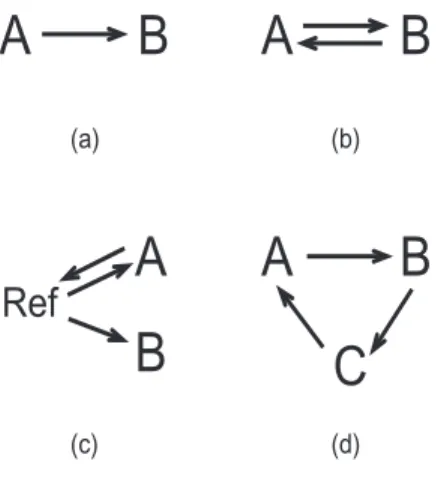
(a) (b) (c) (d)Figure 1: Example designs for two color microarrays.
et al (2002) propose mixed models for single channel oligonucleotide array experiments with multiple probes per gene. The methods of the current paper assume linear models with a single component of variance and so do not apply directly to the mixed model approach, although ideas similar to those used here could be developed. Yang and Speed (2003) and L¨onnstedt et al (2003) take a linear modeling approach similar to that of the current paper.
The plan of this paper is as follows. Section 2 explains the linear modeling approach to the analysis of designed experiments and specifies the response model and distribu-tional assumptions. Section 3 sets out the prior assumptions and defines the posterior variances and moderatedt-statistics. Section 4 derives marginal distributions under the hierarchical model for the observed statistics. Section 5 derives the posterior odds of differential expression and relates it to the t-statistic. The inferential approach based on moderatedt andF statistics is elaborated in Section 6. Section 7 derives estimators for the hyperparameters. Section 8 compares the estimators with earlier statistics in a simulation study. Section 9 illustrates the methodology on two publicly available data sets. Finally, Section 10 makes some remarks on available software.
2
Linear Models for Microarray Data
This section describes how gene-wise linear models arise from experimental designs and states the distributional assumptions about the data which will used in the remainder of the paper. The design of any microarray experiment can be represented in terms of a linear model for each gene. Figure 1 displays some examples of simple designs with two-color arrays using arrow notation as in Kerr and Churchill (2001). Each arrow represents a microarray. The arrow points towards the RNA sample which is labelled red and the sample at the base of the arrow is labelled green. The symbols A, B and C represent RNA sources to be compared. In experiment (a) there is only one microarray which compares RNA sample A and B. For this experiment one can only compute the
log-ratios of expressionyg = log2(Rg)−log2(Gg) whereRg andGg are the red and green
intensities for gene g. Design (b) is a dye-swap experiment leading to a very simple linear model with responses yg1 and yg2 which are log-ratios from the two microarrays and design matrix
X = 1
−1
!
.
The regression coefficient here estimates the contrast B −A on the log-scale, just as for design (a), but with two arrays there is one degree of freedom for error. Design (c) compares samples A and B indirectly through a common reference RNA sample. An appropriate design matrix for this experiment is
X = −1 0 1 0 1 1
which produces a linear model in which the first coefficient estimates the difference betweenAand the reference sample while the second estimates the difference of interest,
B−A. Design (d) is a simple saturated direct design comparing three samples. Different design matrices can obviously be chosen corresponding to different parametrizations. One choice is X = 1 0 0 1 −1 −1
so that the coefficients correspond to the differences B−A and C−B respectively. Unlike two-color microarrays, single color or high density oligonucleotide microarrays usually yield a single expression value for each gene for each array, i.e., competitive hybridization and two color considerations are absent. For such microarrays, design matrices can be formed exactly as in classical linear model practice from the biological factors underlying the experimental layout.
In general we assume that we have a set ofn microarrays yielding a response vector
yTg = (yg1, . . . , ygn) for the gth gene. The responses will usually be log-ratios for
two-color data or log-intensities for single channel data, although other transformations are possible. The responses are assumed to be suitably normalized to remove dye-bias and other technological artifacts; see for example Huber et al (2002) or Smyth and Speed (2003). In the case of high density oligonucleotide array, the probes are assumed to have been normalized to produce an expression summary, represented here as ygi, for
each gene on each array as in Li and Wong (2001) or Irizarry et al (2003). We assume that
E(yg) =Xαg
where X is a design matrix of full column rank and αg is a coefficient vector. We
assume
var(yg) = Wgσg2
where Wg is a known non-negative definite weight matrix. The vector yg may contain
Certain contrasts of the coefficients are assumed to be of biological interest and these are defined by βg = CTα
g. We assume that it is of interest to test whether
individual contrast values βgj are equal to zero. For example, with design (d) above
the experimenter might want to make all the pairwise comparisons B−A, C−B and
C−A which correspond to the contrast matrix
C = 1 0 1 0 1 1
!
There may be more or fewer contrasts than coefficients for the linear model, although if more then the contrasts will be linearly dependent. As another example, consider a simple time course experiment with two single-channel microarrays hybridized with RNA taken at each of the times 0, 1 and 2. If the numbering of the arrays corresponds to time order then we might choose
X = 1 0 0 1 0 0 0 1 0 0 1 0 0 0 1 0 0 1
so thatαgj represents the expression level at the jth time, and
C = −1 0 1 −1 0 1
so that the contrasts measure the change from time 0 to time 1 and from time 1 to time 2 respectively. For an experiment such as this it will most likely be of interest to test the hypothesesβg1 = 0 and βg2 = 0 simultaneously as well as individually because genes with βg1 = βg2 = 0 are those which do not change over time. Composite null hypotheses are addressed in Section 7.
We assume that the linear model is fitted to the responses for each gene to obtain coefficient estimators ˆαg, estimatorss2g of σ2g and estimated covariance matrices
var( ˆαg) =Vgs2g
whereVg is a positive definite matrix not depending ons2g. The contrast estimators are
ˆ
βg =CTαˆg with estimated covariance matrices
var( ˆβg) = CTVgCs2g.
The responsesyg are not necessarily assumed to be normal and the fitting of the linear
model is not assumed to be by least squares. However the contrast estimators are assumed to be approximately normal with mean βg and covariance matrix CTV
and the residual variances s2
g are assumed to follow approximately a scaled chisquare
distribution. The unscaled covariance matrix Vg may depend on αg, for example if
robust regression is used to fit the linear model. If so, the covariance matrix is assumed to be evaluated at ˆαg and the dependence is assumed to be such that it can be ignored
to a first order approximation.
Letvgjbe thejth diagonal element ofCTVgC. The distributional assumptions made
in this paper about the data can be summarized by ˆ βgj|βgj, σ2g ∼N(βgj, vgjσg2) and s2g|σg2 ∼ σ 2 g dg χ2dg
wheredg is the residual degrees of freedom for the linear model for geneg. Under these
assumptions the ordinary t-statistic
tgj = ˆ βgj sg √ vgj
follows an approximatet-distribution on dg degrees of freedom.
The hierarchical model defined in the next section will assume that the estimators ˆ
βg and s2
g from different genes are independent. Although this is not necessarily a
realistic assumption, the methodology which will be derived makes qualitative sense even when the genes are dependent, as they likely will be for data from actual microarray experiments.
This paper focuses on the problem of testing the null hypotheses H0 : βgj = 0 and
aims to develop improved test statistics. In many gene discovery experiments for which microarrays are used the primary aim is to rank the genes in order of evidence against
H0 rather than to assign absolute p-values (Smyth et al, 2003). This is because only a limited number of genes may be followed up for further study regardless of the number which are significant. Even when the above distributional assumptions fail for a given data set it may still be that the tests statistics perform well from a ranking the point of view.
3
Hierarchical Model
Given the large number of gene-wise linear model fits arising from a microarray ex-periment, there is a pressing need to take advantage of the parallel structure whereby the same model is fitted to each gene. This section defines a simple hierarchical model which in effect describes this parallel structure. The key is to describe how the unknown coefficients βgj and unknown variances σg2 vary across genes. This is done by assuming
Prior information is assumed onσ2
g equivalent to a prior estimators20 withd0degrees of freedom, i.e., 1 σ2 g ∼ 1 d0s20 χ2d0.
This describes how the variances are expected to vary across genes. For any given j, we assume that a βgj is non zero with known probability
P(βgj 6= 0) =pj.
Then pj is the expected proportion of truly differentially expressed genes. For those
which are nonzero, prior information on the coefficient is assumed equivalent to a prior observation equal to zero with unscaled variance v0j, i.e.,
βgj|σg2, βgj 6= 0∼N(0, v0jσg2).
This describes the expected distribution of log-fold changes for genes which are differ-entially expressed. Apart from the mixing proportion pj, the above equations describe
a standard conjugate prior for the normal distributional model assumed in the previous section. In the case of replicated single sample data, the model and prior here is a reparametrization of that proposed by L¨onnstedt and Speed (2002). The parametriza-tions are related through dg =f, vg = 1/n, d0 = 2ν, s20 =a/(d0vg) and v0 =cwhere f,
n, ν and a are as in L¨onnstedt and Speed (2002). See also L¨onnstedt (2001). For the calculations in this paper the above prior details are sufficient and it is not necessary to fully specify a multivariate prior for the βg.
Under the above hierarchical model, the posterior mean of σ−2g given s2
g is ˜s −2 g with ˜ s2g = d0s 2 0+dgs2g d0+dg .
The posterior values shrink the observed variances towards the prior values with the degree of shrinkage depending on the relative sizes of the observed and prior degrees of freedom. Define the moderated t-statistic by
˜ tgj = ˆ βgj ˜ sg √ vgj .
This statistic represents a hybrid classical/Bayes approach in which the posterior vari-ance has been substituted into to the classical t-statistic in place of the usual sample variance. The moderated t reduces to the ordinary t-statistic if d0 = 0 and at the opposite end of the spectrum is proportion to the coefficient ˆβgj if d0 =∞.
In the next section the moderated t-statistics ˜tgj and residual sample variances s2g
are shown to be distributed independently. The moderated t is shown to follow a t -distribution under the null hypothesisH0 :βgj = 0 with degrees of freedomdg+d0. The
added degrees of freedom for ˜tgjovertgj reflect the extra information which is borrowed,
on the basis of the hierarchical model, from the ensemble of genes for inference about each individual gene. Note that this distributional result assumesd0 ands20 to be given values. In practice these values need to be estimated from the data as described in Section 6.
4
Marginal Distributions
Section 2 states the distributions of the sufficient statistics ˆβbj ands2g conditional on the
unknown parameters βgj and σg2. Here we derive the unconditional joint distribution
of these statistics under the hierarchical model defined in the previous section. The unconditional distributions are functions of the hyperparameters d0 and s20. It turns out that ˆβgj and s2g are no longer independent under the unconditional distribution
but that ˜tgj and s2g are. For the remainder of this section we will assume that the
calculations are being done for given values ofg and j and for notational simplicity the subscripts g and j will be suppressed in ˜tgj, ˜sg, sg,βgj, vgj,v0j and pj.
It is convenient to note first the density functions for the scaledtandF distributions. If T is distributed as (a/b)1/2Z/U where Z ∼N(0,1) and U ∼χν, then T has density
function
p(t) = a
ν/2b1/2
B(1/2, ν/2)(a+bt2)1/2+ν/2 where B(·,·) is the Beta function. If F is distributed as (a/b)U2
1/U22 where U1 ∼ χ2ν1
and U2 ∼χ2ν2 then F has density function
p(f) = a
ν2/2bν1/2fν1/2−1
B(ν1/2, ν2/2)(a+bf)ν1/2+ν2/2 The null joint distribution of ˆβ and s2 is
p( ˆβ, s2|β = 0) = Z p( ˆβ|σ−2, β = 0)p(s2|σ−2)p(σ−2)d(σ−2) The integrand is 1 (2πvσ2)1/2 exp − ˆ β2 2vσ2 ! × d 2σ2 !d/2 s2(d/2−1) Γ(d/2) exp − ds2 2σ2 ! × d0s 2 0 2 !d0/2 σ−2(d0/2−1) Γ(d0/2) exp −σ−2d0s 2 0 2 ! = (d0s 2 0/2)d0/2(d/2)d/2s2(d/2−1) (2πv)1/2Γ(d 0/2)Γ(d/2) σ−2(1/2+d0/2+d/2−1)exp ( −σ−2 ˆ β2 2v + ds2 2 + d0s20 2 !) which integrates to p( ˆβ, s2|β = 0) = (1/2v) 1/2(d 0s20/2)d0/2(d/2)d/2s2(d/2−1) D(1/2, d0/2, d/2) ˆ β2/v+d0s20+ds2 2 !−(1+d0+d)/2
where D() is the Dirichlet function.
The null joint distribution of ˜t and s2 is
p(˜t, s2|β = 0) = ˜sv1/2p( ˆβ, s2|β = 0) which after collection of factors yields
p(˜t, s2|β = 0) = (d0s 2 0)d0/2dd/2s2(d/2−1) B(d/2, d0/2)(d0s20+ds2)d0/2+d/2 × (d0 +d) −1/2 B(1/2, d0/2 +d/2) 1 + t˜ 2 d0+d !−(1+d0+d)/2
This shows that ˜t and s2 are independent with
s2 ∼s20Fd,d0
and
˜
t|β = 0 ∼td0+d.
The above derivation goes through similarly with β 6= 0, the only difference being that ˜
t|β 6= 0∼(1 +v0/v)1/2td0+d.
The marginal distribution of ˜t over all the genes is therefore a mixture of a scaled
t-distribution and an ordinary t-distribution with mixing proportions p and 1−p re-spectively.
5
Posterior Odds
Given the unconditional distribution of ˜tgj and s2g from the previous section, it is now
easy to compute the posterior odds than any particular geneg is differentially expressed with respect to contrastβgj. The odds that the gth gene has non-zero βgj is
Ogj = p(βgj 6= 0|˜tgj, s2g) p(βgj = 0|˜tgj, s2g) = p(βgj 6= 0, ˜ tgj, s2g) p(βgj = 0,t˜gj, s2g) = pj 1−pj p(˜tgj|βgj 6= 0) p(˜tgj|βgj = 0)
since ˜tgj and s2g are independent and the distribution of s2g does not depend on βgj.
Substituting the density for ˜tgj from Section 4 gives
Ogj = pj 1−pj vgj vgj+v0j !1/2 ˜ t2 gj+d0 +dg ˜ t2 gj vgj vgj+v0j +d0+dg (1+d0+dg)/2
This agrees with equation (7) of L¨onnstedt and Speed (2002). In the limit for d0 +dg
large, the odds ratio reduces to
Ogj = pj 1−pj vgj vgj+v0j !1/2 exp ˜ t2gj 2 v0j vgj+v0j ! .
This expression is important for accurate computation ofOgj in limiting cases.
Follow-ing L¨onnstedt and Speed (2002), the statistic
Bgj = logOgj
is on a friendly scale and is useful for ranking genes in order of evidence for differential expression. Note that Bgj is monotonic increasing in |˜tgj| if the dg and vg do not vary
between genes.
6
Estimation of Hyperparameters
6.1
General
The statistics Bgj and ˜tgj depend on the hyperparameters in the hierachical model
defined in Section 3. A fully Bayesian approach would be to allow the user to choose these parameters. This paper takes instead an empirical Bayes approach in which these parameters are estimated from the data. The purpose of this section is to develop consistent, closed form estimators for d0, s0 and the v0j from the observed sample
variancess2g and moderatedt-statistics ˜tgj. We estimate d0 ands20 from thes2g and then
estimate thev0j from the ˜tgj assuming d0 and thepj to be known.
Specifically, d0 and s20 are estimated by equating empirical to expected values for the first two moments of logs2g. We use logs2g here instead ofs2g because the moments of logs2
g are finite for any degrees of freedom and because the distribution of logs2g is more
nearly normal so that moment estimation is likely to be more efficient. We estimate the v0j by equating the order statistics of the|t˜gj| to their nominal values. Each order
statistic of the |˜tgj| yields an individual estimator of v0j. A final estimator of v0j is obtained by averaging the estimators arising from the topGpj/2 of the order statistics
where Gis the number of genes.
The closed form estimators given here could be used as starting values for maximum likelihood estimation of d0, s0 and the v0j based on the marginal distributions of the
observed statistics, although that route is not followed in this paper. The large size of microarray data sets ensures that the moment estimators given here are reasonably precise without further iteration.
6.2
Estimation of
d
0and
s
0Write
zg = logs2g
Each s2
g follows a scaled F-distribution so zg is distributed as a constant plus Fisher’s
z distribution (Johnson and Kotz, 1970, page 78). The distribution of zg is roughly
normal and has finite moments of all orders including
and
var(zg) = ψ0(dg/2) +ψ0(d0/2)
where ψ() andψ0() are the digamma and trigamma functions respectively. Write
eg =zg−ψ(dg/2) + log(dg/2)
Then
E(eg) = logs20−ψ(d0/2) + log(d0/2) and
E{(eg−e¯)2G/(G−1)−ψ0(dg/2)} ≈ψ0(d0/2) We can therefore estimated0 by solving
ψ0(d0/2) = mean
n
(eg−e¯)2G/(G−1)−ψ0(dg/2)
o
(1) for d0. Although the inverse of the trigamma function is not a standard mathematical function, equation (1) can be solved very efficiently using a monotonically convergent Newton iteration as described in the appendix.
Given an estimate for d0,s20 can be estimated by
s20 = exp{¯e+ψ(d0/2)−log(d0/2)} This estimate for s2
0 is usually somewhat less than the mean of the s2g in recognition of
the skewness of the F-distribution.
Note that these estimators allow for dg to differ between genes and therefore allow
for arbitrary missing values in the expression data. Note also that any gene for which
dg = 0 will receive ˜s2g =s20.
In the case that mean{(eg−e¯)2G/(G−1)−ψ0(dg/2)} ≤ 0, (1) cannot be solved
because the variability of the s2
g is less than or equal to that expected from chisquare
sampling variability. In that case there is no evidence that the underlying variancesσ2
g
vary between genes so d0 is set to positive infinity and s20 = exp(¯e).
6.3
Estimation of
v
0jIn this section we consider the estimation of the v0j for a givenj. For ease of notation,
the subscriptj will be omitted from ˜tgj,vgj,v0j andpj for the remainder of this section.
Gene g yields a moderated t-statistic ˜tg. The cumulative distribution function of ˜tg
is F(˜tg; vg, v0, d0+dg) = pF ˜tg ( vg vg +v0 )1/2 ; d0 +dg + (1−p)F ˜ tg; d0+dg
whereF(·; k) is the cumulative distribution function of the t-distribution on k degrees of freedom. Let r be the rank of gene g when the |˜tg| are sorted in descending order.
We match thep-value of any particular|˜tg| to its nominal value given its rank. For any particular gene g and rankr we need to solve
2F(−|t˜g|; vg, v0, d0+dg) = r−0.5
G (2)
forv0. The left-hand side is the actualp-value given the parameters and the right-hand side is the nominal value for the p-value of rank r. The interpretation is that, if a probability plot was constructed by plotting the |˜tg| against the theoretical quantiles corresponding to probabilities (r−0.5)/G, (2) is the condition that a particular value of |˜tg| will lie exactly on the line of equality. The value of v0 which solves (2) is
v0 =vg ˜ t2 g q2 target −1 ! with qtarget =F−1(ptarget; d0+dg) and ptarget = 1 p r−0.5 2G −(1−p)F(−|˜tg|;d0+dg)
provided that 0< ptarget <1 and qtarget ≤ |˜tg|.
If |˜tg| lies above the line of equality in a t-distribution probability plot, i.e., if
F(−|t˜g|;d0+dg)<(r−0.5)/(2G), thenptarget >0 andv0 >0. Restricting to those val-ues of rfor which (r−0.5)/(2G)< p ensures also that ptarget <1 so that the estimator of v0 is defined. If |˜tg|does not lie above the line of equality then the best estimate for
v0 is zero.
To get a combined estimator of v0, we obtain individual estimators of v0 for r = 1, . . . , Gp/2 and set v0 to be the mean of these estimators. The combined estimator will be positive, unless none of the top Gp/2 values for |˜tg| exceed the corresponding order statistics of thet-distribution, in which case the estimator will be zero.
6.4
Practical Considerations: Estimation of
p
jIn principle it is not difficult to estimate the proportions pj from the data as well as
the other hyperparameters. A natural estimator would be to iteratively set
pj = 1 G G X i=1 Ogj 1 +Ogj
since Ogj/(1 +Ogj) is the estimated probability that gene g is differentially expressed,
and there are other possibilities such as maximum likelihood estimation. The data however contain considerably more information aboutd0 and s20 than about thev0j and
the pj. This is because all the genes contribute to estimation ofd0 and s20 whereas only those which are differential expressed contribute to estimation of v0j or pj, and even
Any set of sample variances s2
g leads to useful estimates of d0 and s20. On the other hand, the estimation ofv0j and pj is somewhat unstable in that estimates on the
boundaries pj = 0, pj = 1 or v0j = 0 have positive probability and these boundary
values lead to degenerate values for the posterior odds statisticsBgj. Even when not on
the boundary, the estimator for pj is likely to be sensitive to the particular form of the
prior distribution assumed for βgj and possibly also to dependence between the genes
(Ferkingstad et al, 2003).
A practical strategy to bypass these problems is to set the pj to values chosen by
the user, perhaps pj = 0.01 or some other small value. Since v
1/2
0j σg is the standard
deviation of the log-fold-changes for differentially expressed genes, and because this standard deviation cannot be unreasonably small or large in a microarray experiment, it seems reasonable to place some prior bounds onv01/j2s0as well. In the software package Limma which implements the methods in this paper, the user is allowed to place limits on the possible values forv10j/2s0. By default these limits are set at 0.1 and 4, chosen to include a wide range of reasonable values. For many data sets these limits do not come into play but they do prevent very small or very large estimated values for v0j.
7
Inference Using Moderated
t
and
F
Statistics
As already noted, the odds ratio statistic for differential expression derived in Section 5 is monotonic increasing in|˜tgj|for any givenj ifdg andvg do not vary between genes. This shows that the moderatedt-statistic is an appropriate statistic for assessing differential expression and is equivalent toBgj as a means of ranking genes. Even when dg and vg
do vary, it is likely that p-values from the ˜tgj will rank the genes in very similar order
to the Bgj.
The moderated t has the advantage over the B-statistic that Bgj depends on
hy-perparameters v0j and pj for all j as well as d0 and s20 whereas ˜tgj depends only on d0 ands2
0. This means that the moderated tdoes not require knowledge of the proportion of differentially expressed genes, a potentially contentious parameter, nor does it make any assumptions about the magnitude of differential expression when it exists. The moderated t does require knowledge of d0 and s20, which describe the variability of the true gene-wise variances, but these hyperparameters can be estimated in stable fashion as described in Section 6.
The moderatedt has the advantage over the ordinaryt statistic that large statistics are less likely to arise merely from under-estimated sample variances. This is because the posterior variance ˜s2g offsets the small sample variances heavily in a relative sense while larger sample variances are moderated to a lesser relative degree. In this respect the moderatedtstatistic is similar in spirit tot-statistics with offset standard deviation. Provided thatd0 <∞ and dg >0, the moderated t-statistic can be written
˜ tgj = d0+dg dg !1/2 ˆ βgj q s2 ∗,gvgj
wheres2
∗,g =s2g+ (d0/dg)s20. This shows that the moderatedt-statistic is proportional to at-statistic with sample variances offset by a constant if thedg are equal. Test statistics
with offset standard deviations of the form
t∗,gj = ˆ βgj (sg+a) √ vgj ,
whereais a positive constant, have been used by Tusher et al (2001), Efron et al (2001) and Broberg (2003). Note that t∗ offsets the standard deviation while ˜t offsets the variance so the two statistics are not functions of one another. Unlike the moderated
t, the offset statistic t∗,gj is not connected in any formal way with the posterior odds of
differential expression and does not have an associated distributional theory.
The moderatedt-statistic ˜tgjmay be used for inference aboutβgj in a similar way to
that in which the ordinaryt-statistic would be used, except that the degrees of freedom are dg+d0 instead of dg. The fact that the hyperparameters d0 and s20 are estimated from the data does not impact greatly on the individual test statistics because the hyperparameters are estimated using data from all the genes, meaning that they are estimated relatively precisely and can be taken to be known at the individual gene level. The moderated t-statistics also lead naturally to moderated F-statistics which can be used to test hypotheses about any set of contrasts simultaneously. Appropriate quadratic forms of moderated t-statistics follow F-distributions just as do quadratic forms of ordinaryt-statistics. Suppose that we wish to test all contrasts for a given gene equal to zero, i.e., H0 : βg = 0. The correlation matrix of ˆβg is Rg =Ug−1CTVgCUg−1
where Ug is the diagonal matrix with unscaled standard deviations (vgj)1/2 on the
di-agonal. Let r be the column rank of C. Let Qg be such that QTgRgQg = Ir and let
qg =QTgtg. Then
Fg =qTgqg/r=tTgQgQTgtg/r∼Fr,d0+dg
If we choose the columns of Qg to be the eigenvectors spanning the range space of Rg
then QTgRgQg = Λg is a diagonal matrix and
Fg =qTgΛ
−1
g qg/r ∼Fr,d0+dg.
The statistic Fg is simply the usual F-statistic from linear model theory for testing βg = 0 but with the posterior variance ˜s2g substituted for the sample variances2g in the denominator.
8
Simulation Results
This section presents a simulation study comparing the moderatedt-statistic with four other statistics for ranking genes in terms of evidence for differential expression. The moderated t statistic is compared with (i) ordinary fold change, equivalent to |βˆgj|,
(ii) the ordinary t-statistic |tgj|, (iii) Efron’s idea of offsetting the standard deviations
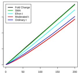
0 50 100 150 200 0 50 100 150 N Genes Selected N False Discoveries Fold Change SMA Efron t Moderated t Ordinary t Variances Different
Figure 2: False discovery rates for different gene selection statistics when the true variances are very different, i.e., the residual variance dominates. The rates are means of actual false discovery rates for 100 simulated data sets.
0 50 100 150 200 0 50 100 150 N Genes Selected N False Discoveries Fold Change SMA Efron t Moderated t Ordinary t Variances Balanced
Figure 3: False discovery rates for different gene selection statistics when the true variances are somewhat different, i.e., the prior and residual degrees of freedom are balanced. The rates are means of actual false discovery rates for 100 simulated data sets.
0 50 100 150 200 0 50 100 150 N Genes Selected N False Discoveries Fold Change SMA Efron t Moderated t Ordinary t Variances Similar
Figure 4: False discovery rates for different gene selection statistics when the true variances are somewhat different, i.e., the prior and residual degrees of freedom are balanced. The rates are means of actual false discovery rates for 100 simulated data sets.
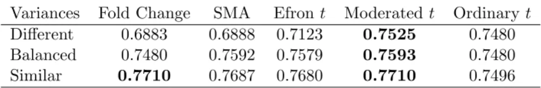
Table 1: Area under the Receiver Operating Curve for five statistics and three simulation scenarios.
Variances Fold Change SMA Efront Moderated t Ordinary t
Different 0.6883 0.6888 0.7123 0.7525 0.7480
Balanced 0.7480 0.7592 0.7579 0.7593 0.7480
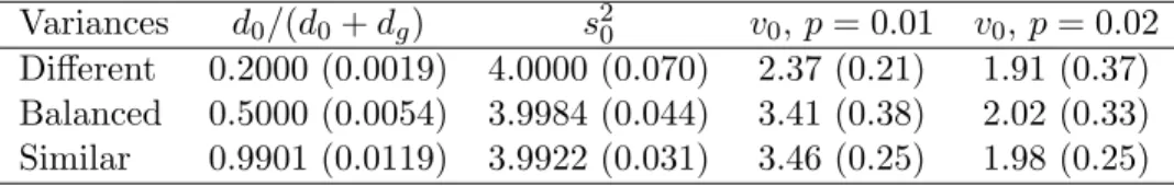
Table 2: Means (standard deviations) of hyperparameter estimates for the simulated data sets. True values ared0/(d0+dg) = 0.2,0.5,0.9960,s20 = 4,v0 = 2.
Variances d0/(d0+dg) s20 v0,p= 0.01 v0,p= 0.02
Different 0.2000 (0.0019) 4.0000 (0.070) 2.37 (0.21) 1.91 (0.37) Balanced 0.5000 (0.0054) 3.9984 (0.044) 3.41 (0.38) 2.02 (0.33) Similar 0.9901 (0.0119) 3.9922 (0.031) 3.46 (0.25) 1.98 (0.25)
implemented in the SMA package for R. For Efron’s offsett-statistic we select genes in order of |tE,gj|where
tE,gj = ˆ βgj (sg+s0.9) √ vgj
wheres0.9 is the 90th percentile of thesg. This is corresponds to the statistic defined by
Efron et al (2001). For the L¨onnstedt and Speed (2002) method, genes were selected in order of the B-statistic or log-odds computed by the stat.bay.est function the SMA package for R available from
http://www.stat.berkeley.edu/users/terry/zarray/Software/smacode.html.
The L¨onnstedt and Speed (2002) B-statistic is equivalent here to the moderated t
except for differences in the hyperparameter estimators. The moderated t-statistic was evaluated at the hyperparameter estimators derived in Section 6.
Data sets were simulated from the hierarchical model of Section 3 under three dif-ferent parameter scenarios, one where the gene-wise variances are quite difdif-ferent, one where prior and residual degrees of freedom are balanced and one where the gene-wise variances are nearly constant. Data sets were simulated with 15000 genes, 300 or p = 0.02 of which were differentially expressed. All three scenarios used dg = 4,
s2
0 = 4, vg = 1/3 and v0 = 2. The prior degrees of freedom was varied between the scenarios with d0 = 1 for the scenario with very different variances, d0 = 4 to balance the prior and residual degrees of freedom and d0 = 1000 to make the true variances almost identical. A hundred data sets were simulated for each scenario.
Figures 2-4 plot the average false discovery rates for the five statistics and Table 1 gives the areas under the receiver operating curves (ROCs). The moderated t-statistic has the lowest false discovery rate and the highest area under the ROC for all three scenarios. The straight fold change does equally well, as expected, when the true variances are nearly constant. The SMA B-statistic and Efron’s t statistic do nearly as well as the moderated t statistic when the prior and residual degrees of freedom are balanced but they are less able to adapt to other arrangements for the true variances. Although the moderatedt can be expected to perform better than the fold change and the ordinary t-statistic on data simulated under the assumed hierarchical model, the simulations show that this advantage is realized even though the hyperparameters need to be estimated.
Table 2 give means and standard deviations of the hyperparameter estimates for the simulated data sets. The estimates for d0/(d0 +dg) and s20 were very accurate. The estimator for v0 was nearly unbiased when p was set to the true proportion of differentially expressed genes (p = 0.02) but was somewhat over-estimated when the proportion was set to a lower value (p = 0.01). As expected the estimator for v0 is somewhat more variable than that ofd0/(d0 +dg) or s20. The results shown in Table 2 are not affected by the prior limits on v0s20 discussed in Section 6.
9
Data Examples
9.1
Swirl
Consider the Swirl data set which is distributed as part of the marrayInput package for R (Dudoit and Yang, 2003). The experiment was carried out using zebrafish as a model organism to study the early development in vertebrates. Swirl is a point mutant in the BMP2 gene that affects the dorsal/ventral body axis. The main goal of the Swirl experiment is to identify genes with altered expression in the Swirl mutant compared to wild-type zebrafish. The experiment used four arrays in two dye-swap pairs. The microarrays used in this experiment were printed with 8448 probes (spots) including 768 control spots. The hybridized microarrays were scanned with an Axon scanner and SPOT image analysis software (Buckley, 2000) was used to capture red and green intensities for each spot. The data was normalized using print-tip loess normalization and between arrays scale normalization using the LIMMA package (Smyth, 2003). Loess normalization used window span 0.3 and three robustifying iterations.
For this data all genes have dg = 3 and vg = 1/4. The estimated prior degrees
of freedom are d0 = 4.17 showing that posterior variances will be balanced between the prior and sample variances with only slightly more weight to the former. The estimated prior variance is s2
0 = 0.0509 which is less then the mean variance at 0.109 but more than the median at 0.047. The estimated unscaled variance for the contrast is v0 = 22.7, meaning that the standard deviation of the log-ratio for a typical gene is (0.0509)1/2(22.7)1/2 = 1.07, i.e., genes which are differentially expressed typically change by about two-fold. The prior limits on v0s20 discussed in Section 6 do not come into play for this data. The proportion of differentially expressed genes was set to p= 0.01 following the default in the earlier SMA software. This value seems broadly realistic for single-gene knock-out vs wild-type experiments but is probably conservative for other experiments where more differential expression is expected.
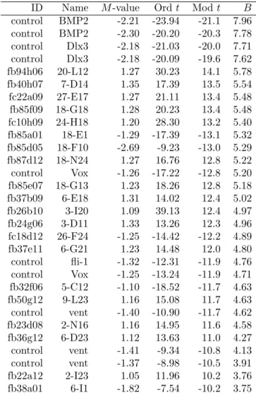
Table 3 shows the top 30 genes as ranked by the B-statistic. The table includes the fold change (or M-value), the ordinary t-statistic, the moderated t-statistic and the B-statistic for the each gene. The moderated t and the B-statistics are evaluated at the hyperparameter estimators derived in Section 6. There are no missing values for this data so the two statistics necessarily give the same ranking of the genes. The ordinaryt-statistics are on 3 degrees of freedom while the moderatedtare on 7.17. The moderated t-statistic method here ranks both copies of the knock-out gene BMP2 first
Table 3: Top 30 genes from the Swirl data
ID Name M-value Ordt Modt B
control BMP2 -2.21 -23.94 -21.1 7.96 control BMP2 -2.30 -20.20 -20.3 7.78 control Dlx3 -2.18 -21.03 -20.0 7.71 control Dlx3 -2.18 -20.09 -19.6 7.62 fb94h06 20-L12 1.27 30.23 14.1 5.78 fb40h07 7-D14 1.35 17.39 13.5 5.54 fc22a09 27-E17 1.27 21.11 13.4 5.48 fb85f09 18-G18 1.28 20.23 13.4 5.48 fc10h09 24-H18 1.20 28.30 13.2 5.40 fb85a01 18-E1 -1.29 -17.39 -13.1 5.32 fb85d05 18-F10 -2.69 -9.23 -13.0 5.29 fb87d12 18-N24 1.27 16.76 12.8 5.22 control Vox -1.26 -17.22 -12.8 5.20 fb85e07 18-G13 1.23 18.26 12.8 5.18 fb37b09 6-E18 1.31 14.02 12.4 5.02 fb26b10 3-I20 1.09 39.13 12.4 4.97 fb24g06 3-D11 1.33 13.26 12.3 4.96 fc18d12 26-F24 -1.25 -14.42 -12.2 4.89 fb37e11 6-G21 1.23 14.48 12.0 4.80 control fli-1 -1.32 -12.31 -11.9 4.76 control Vox -1.25 -13.24 -11.9 4.71 fb32f06 5-C12 -1.10 -18.52 -11.7 4.63 fb50g12 9-L23 1.16 15.08 11.7 4.63 control vent -1.40 -10.90 -11.7 4.62 fb23d08 2-N16 1.16 14.95 11.6 4.58 fb36g12 6-D23 1.12 13.63 11.0 4.27 control vent -1.41 -9.34 -10.8 4.13 control vent -1.37 -8.98 -10.5 3.91 fb22a12 2-I23 1.05 11.96 10.2 3.76 fb38a01 6-I1 -1.82 -7.54 -10.2 3.75
and both copies of Dlx3, which is a known target of BMP2, second. Neither the fold change nor the ordinary t-statistic do this. In general the moderated methods give a more predictable ranking of the control genes.
9.2
ApoAI
These data are from a study of lipid metabolism by Callow et al (2000) and are available from
http://www.stat.berkeley.edu/users/terry/zarray/Html/matt.html.
The apolipoprotein AI (ApoAI) gene is known to play a pivotal role in high density lipoprotein (HDL) metabolism. Mouse which have the ApoAI gene knocked out have very low HDL cholesterol levels. The purpose of this experiment is to determine how ApoAI deficiency affects the action of other genes in the liver, with the idea that this will help determine the molecular pathways through which ApoAI operates.
The experiment compared 8 ApoAI knockout mice with 8 normal C57BL/6 mice, the control mice. For each of these 16 mice, target mRNA was obtained from liver tissue and labelled using a Cy5 dye. The RNA from each mouse was hybridized to a separate microarray. Common reference RNA was labelled with Cy3 dye and used for all the arrays. The reference RNA was obtained by pooling RNA extracted from the 8 control mice. Although still a simple design, this experiment takes us outside the replicated array structure considered by L¨onnstedt and Speed (2002).
Intensity data was captured from the array images using SPOT software and the data was normalized using print-tip loess normalization. The normalized intensities were analyzed for differential expression by fitting a two-parameter linear model, the parameter of interest measuring the difference between the ApoAI knockout line and the control mice.
The residual degrees of freedom aredg = 14 for most genes but some havedg as low
as 10. The estimated prior degrees of freedom are d0 = 3.7. The residual degrees of freedom are relatively large here so the sample variances will be shrunk only slightly and the moderated and ordinary t-statistics will differ substantially only when the sample variance is unusually small. The prior variance is s2
0 = 0.048 which is somewhat less than the median sample variance at 0.064. The unscaled variance for the contrasts of interest is estimated to bev0 = 3.4 meaning that the typical fold change for differentially expressed genes is estimated to be about 1.3. Prior limits onv0s20 do not come into play for these data.
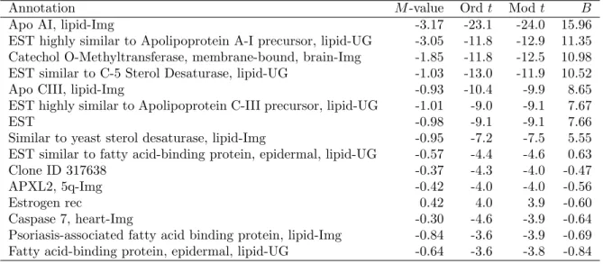
Table 4 shows the top 15 genes as ranked by the B-statistic for the parameter of interest. The moderated t rank the genes in the same order even though there are a few missing values for this data. The top gene is ApoAI itself which is heavily down-regulated as expected. Several of the other genes are closely related to ApoAI. The top eight genes here have been confirmed to be differentially expressed in the knockout versus the control line (Callow et al, 2000). For these data the top eight genes stand out clearly from the other genes and all methods clearly separate these genes from the
Table 4: Top 15 genes from the ApoAI data
Annotation M-value Ordt Modt B
Apo AI, lipid-Img -3.17 -23.1 -24.0 15.96 EST highly similar to Apolipoprotein A-I precursor, lipid-UG -3.05 -11.8 -12.9 11.35 Catechol O-Methyltransferase, membrane-bound, brain-Img -1.85 -11.8 -12.5 10.98 EST similar to C-5 Sterol Desaturase, lipid-UG -1.03 -13.0 -11.9 10.52 Apo CIII, lipid-Img -0.93 -10.4 -9.9 8.65 EST highly similar to Apolipoprotein C-III precursor, lipid-UG -1.01 -9.0 -9.1 7.67
EST -0.98 -9.1 -9.1 7.66
Similar to yeast sterol desaturase, lipid-Img -0.95 -7.2 -7.5 5.55 EST similar to fatty acid-binding protein, epidermal, lipid-UG -0.57 -4.4 -4.6 0.63 Clone ID 317638 -0.37 -4.3 -4.0 -0.47 APXL2, 5q-Img -0.42 -4.0 -4.0 -0.56 Estrogen rec 0.42 4.0 3.9 -0.60 Caspase 7, heart-Img -0.30 -4.6 -3.9 -0.64 Psoriasis-associated fatty acid binding protein, lipid-Img -0.84 -3.6 -3.9 -0.69 Fatty acid-binding protein, epidermal, lipid-UG -0.64 -3.6 -3.8 -0.84
others. The B-statistic for example drops from 5.55 to 0.63 from the 8th to the 9th ranked gene.
10
Software
The methods described in this paper, including linear models and contrasts as well as moderated t and F statistics and posterior odds, are implemented in the software package Limma for the R computing environment (Smyth et al, 2003). Limma is part of the Bioconductor project at http://www.bioconductor.org (Gentleman et al, 2003). The Limma software has been tested on a wide range of microarray data sets from many different facilities and has been used routinely at the author’s institution since the middle of 2002.
Colophon
The author thanks Terry Speed, Ingrid L¨onnstedt, Yu Chuan Tai and Turid Follestad for valuable discussions and for comments on an earlier version of this manuscript. Thanks also to Suzanne Thomas for assistance with the figures. This research was supported by NHMRC Grants 257501 and 257529.
Appendix: Inversion of Trigamma Function
In this appendix we solve ψ0(y) =x for y where x > 0 by deriving a Newton iteration with guaranteed and rapid convergence.
Define f(y) = 1/ψ0(y). The function f is nearly linear and convex for y > 0, satisfying f(0) = 0 and asymptoting to f(y) =y−0.5 as y→ ∞. The first derivative
f0(y) = −ψ
00(y)
ψ0(y)2
is strictly increasing fromf0(0) = 0 tof0(∞) = 1. This means that the Newton iteration to solvef(y) =z for y is monotonically convergent provided that the starting value y0 satisfiesf(y0)≥z. Such a starting value is provided by y0 = 0.5 +z.
The complete Newton iteration to solveψ0(y) =x is as follows. Set y0 = 0.5 + 1/x. Then iterate yi+1 =yi+δi with δi =ψ0(yi){1−ψ0(yi)/x}/ψ00(yi) until−δi/y < where
is a small positive number. The step δi is strictly negative unless ψ0(yi) = x. Using
64-bit double precision arithmetic, = 10−8 is adequate to achieve close to machine precision accuracy. To avoid overflow or underflow in floating point arithmetic, we can set y = 1/√x when x > 107 and y = 1/x when x < 10−6 instead of performing the iteration. Again these choices are adequate for nearly full precision in 64-bit arithmetic.
References
Baldi, P., and Long, A. D. (2001). A Bayesian framework for the analysis of microar-ray expression data: regularized t-test and statistical inferences of gene changes.
Bioinformatics 17, 509–519.
Broberg, P. (2003). Statistical methods for ranking differentially expressed genes.
Genome Biology 4: R41.
Buckley, M. J. (2000). Spot User’s Guide. CSIRO Mathematical and Information Sciences, Sydney, Australia. http://www.cmis.csiro.au/iap/Spot/spotmanual.htm. Callow, M. J., Dudoit, S., Gong, E. L., Speed, T. P., and Rubin, E. M. (2000).
Mi-croarray expression profiling identifies genes with altered expression in HDL deficient mice. Genome Research 10, 2022–2029.
Chu, T.-M., Weir, B., and Wolfinger, R. (2002). A systematic statistical linear modeling approach to oligonucleotide array experiments. Mathematical Biosciences 176, 35– 51.
Cui, X., and Churchill, G. A. (2003). Statistical tests for differential expression in cDNA microarray experiments. Genome Biology 4, 210.1–210.9.
Dudoit, S., and Yang, Y. H. (2003). Bioconductor R packages for exploratory analysis and normalization of cDNA microarray data. In G. Parmigiani, E. S. Garrett, R. A.
Irizarry and S. L. Zeger, editors, The Analysis of Gene Expression Data: Methods
and Software, Springer, New York. pp. 73-101.
Efron, B. (2003). Robbins, empirical Bayes and microarrays. Annals of Statistics 31, 366–378.
Efron B., Tibshirani, R., Storey J. D., and Tusher V. (2001). Empirical Bayes analysis of a microarray experiment. Journal of the American Statistical Association 96, 1151–1160.
Ferkingstad, E., Langaas, M., and Lindqvist, B. (2003). Estimating the proportion of true null hypotheses, with application to DNA microarray data. Preprint Statistics No. 4/2003, Norwegian University of Science and Technology, Trondheim, Norway. http://www.math.ntnu.no/preprint/
Ge, Y., Dudoit, S., and Speed, T. P. (2003). Resampling-based multiple testing for microarray data analysis, with discussion. TEST 12, 1–78.
Gentleman, R., Bates, D., Bolstad, B., Carey, V., Dettling, M., Dudoit, S., Ellis, B., Gautier, L., Gentry, J., Hornik, K., Hothorn, T., Huber, W., Iacus, S., Irizarry, R., Leisch, F., C., Maechler, M., Rossini, A. J., Sawitzki, G., Smyth, G. K., Tierney, L., Yang, J. Y. H., and Zhang, J. (2003). Bioconductor: a software development project. Technical Report November 2003, Department of Biostatistics, Harvard School of Public Health, Boston.
Huber, W., von Heydebreck, A., Sltmann, H., Poustka, A., and Vingron, M. (2002). Variance stabilization applied to microarray data calibration and to the quantifica-tion of differential expression. Bioinformatics 18, S96–S104.
Ibrahim, J. G., Chen, M.-H., and Gray, R. J. (2002). Bayesian models for gene expres-sion with DNA microarray data. Journal of the American Statistical Society 97, 88-99.
Irizarry, R. A., Bolstad, B. M., Francois Collin, F., Cope, L. M., Hobbs, B., and Speed, T. P. (2003), Summaries of Affymetrix GeneChip probe level data. Nucleic Acids Research 31(4):e15.
Jin, W., Riley, R. M., Wolfinger, R. D., White, K. P., Passador-Gurgel, G., and Gibson, G. (2001). The contributions of sex, genotype and age to transcriptional variance in Drosophila melanogaster. Nature Genetics 29, 389–395.
Johnson, N. L., and Kotz, S. (1970). Distributions in Statistics: Continuous Univariate
Distributions – 2. Wiley, New York.
Kendziorski, C. M., Newton, M. A., Lan, H., and Gould, M. N. (2003). On paramet-ric empiparamet-rical Bayes methods for comparing multiple groups using replicated gene expression profiles. Statistics in Medicine 22, 3899–3914.
Kerr, M. K., and Churchill, G. A. (2001). Experimental design for gene expression microarrays. Biostatistics 2, 183–201.
Kerr, M. K., Martin, M., and Churchill, G. A. (2000). Analysis of variance for gene expression microarray data. Journal of Computational Biology 7, 819–837.
Li, C., and Wong, W. H. (2001). Model-based analysis of oligonucleotide arrays: expres-sion index computation and outlier detection. Proceedings of the National Academy of Sciences 98, 31–36.
L¨onnstedt, I. (2001). Replicated Microarray Data. Licentiate Thesis, Department of Mathematics, Uppsala University.
L¨onnstedt, I., Grant, S., Begley, G., and Speed, T. P. (2003). Microarray analysis of two interacting treatments: a linear model and trends in expression over time. Technical Report, Department of Mathematics, Uppsala University.
L¨onnstedt, I., and Speed, T. P. (2002). Replicated microarray data. Statistica Sinica
12, 31–46.
Nature Genetics Editors (eds.) (2003). Chipping Forecast II. Nature Genetics Supple-ment 32, 461–552.
Newton, M.A. and Kendziorski, C. M. (2003). Parametric empirical Bayes methods for microarrays. In: The analysis of gene expression data: methods and software. Eds. G. Parmigiani, E. S. Garrett, R. Irizarry and S. L. Zeger, Springer Verlag, New York. To appear.
Newton, M. A., Kenziorski, C. M., Richmond, C. S., Blattner, F. R., and Tsui, K. W. (2001). On differential variability of expression ratios: improving statistical inference about gene expression changes from microarray data. Journal of Computational Biology 8, 37–52.
Parmigiani, G., Garrett, E. S., Irizarry, R. A., and Zeger, S. L. (eds.) (2003). The
Analysis of Gene Expression Data: Methods and Software. Springer, New York.
Smyth, G. K., Thorne, N. P., and Wettenhall, J. (2003). Limma: Linear Models for
Mi-croarray Data User’s Guide. Software manual available from
http://www.biocond-uctor.org.
Smyth, G. K., and Speed, T. P. (2003). Normalization of cDNA microarray data.
Methods 31, 265–273.
Smyth, G. K., Yang, Y.-H., Speed, T. P. (2003). Statistical issues in cDNA microarray data analysis. Methods in Molecular Biology 224, 111–136.
Speed, T. P. (ed.) (2003). Statistical Analysis of Gene Expression Microarray Data. Chapman & Hall/CRC, Boca Raton.
Tusher, V. G., Tibshirani, R., and Chu, G. (2001). Significance analysis of microarrays applied to the ionizing radiation response. PNAS98, 5116–5121.
Wolfinger, R. D., Gibson, G., Wolfinger, E. D., Bennett, L., Hamadeh, H., Bushel, P., Afshari, C., and Paules, R. S. (2001). Assessing gene significance from cDNA microarray expression data via mixed models. Journal of Computational Biology8, 625–637.
Yang, Y. H., and Speed, T. P. (2003). Design and analysis of comparative microarray experiments. In T. P. Speed (ed.),Statistical Analysis of Gene Expression