Portable Data Mining on Azure and HPC Platform

(1)

Judy Qiu, Thilina Gunarathne, Bingjing Zhang, Xiaoming Gao, Fei Teng

SALSA HPC Group

http://salsahpc.indiana.edu

School of Informatics and Computing Indiana University

Portable Data Mining

(2)

Data Intensive Iterative Applications

• Growing class of applications

–

Clustering, data mining, machine learning & dimension

reduction applications Expectation Maximization

–

Driven by data deluge & emerging computation fields

–

Lots of scientific applications

k ← 0;

MAX ← maximum iterations δ[0] _{← initial delta value}

while ( k< MAX_ITER || f(δ[k]_{, δ}[k-1]_{) )}

foreach datum in data

β[datum] ← process (datum, δ[k]₎

end foreach

δ[k+1]_{← combine(β[])}

k ← k+1

(3)

(4)

Data Intensive Iterative Applications

• Common Characteristics

• Compute (map) followed by LARGE

communication Collectives (reduce)

Compute Communication Reduce/ barrier

New Iteration Larger Loop-Invariant Data Smaller Loop-Variant Data Broadcast

(5)

Iterative MapReduce

• MapReduceMerge

• Extensions to support additional broadcast (+other)

input data

Map(<key>, <value>, list_of <key,value>)

Reduce(<key>, list_of <value>, list_of <key,value>) Merge(list_of <key,list_of<value>>,list_of <key,value>)

(6)

Parallel Data Analysis using Twister

Data mining and Data analysis Applications

Next Generation Sequencing Image processing Search Engine ….

Algorithms

Multidimensional Scaling (MDS) Clustering (K-means) Indexing ….

(7)

Traditional MapReduce and classical parallel

runtimes cannot solve iterative algorithms

efficiently

Hadoop: Repeated data access to HDFS, no optimization to data caching and data transfers

MPI: no natural support of fault tolerance and programming interface is complicated

Interoperability

(8)

Current and Future Work

Collective Communication

Fault tolerance

Distributed Storage

High level language

(9)

Twister Collective Communications

 Broadcasting

 Data could be large

 Chain & MST

 Map Collectives  Local merge

 Reduce Collectives  Collect but no merge

 Combine

 Direct download or Gather

Map Tasks Map Tasks

Map Collective Reduce Tasks Reduce Collective Gather Map Collective Reduce Tasks Reduce Collective Map Tasks Map Collective Reduce Tasks Reduce Collective Broadcast

(10)

Twister Broadcast Comparison

One-to-All vs. All-to-All implementations

0 100 200 300 400 500

Per Iteration Cost (Before) Per Iteration Cost (After)

Time (Unit:

Sec

ond

s)

(11)

0 5 10 15 20 25 1 25 50 75 100 125 150 Bc as t Time (Se con d s) Number of Nodes

Twister Bcast 500MB MPI Bcast 500MB Twister Bcast 1GB

MPI Bcast 1GB Twister Bcast 2GB MPI Bcast 2GB

Bcast Byte Array on PolarGrid (Fat-Tree Topology

with 1Gbps Ethernet):

Twister v. MPI (OpenMPI)

(12)

Collective algorithm uses

Topology-aware Pipeline

Core Switch Compute Node Rack Switch Compute Node Compute Node pg1-pg42 1 Gbps Connection 10 Gbps Connection Compute Node Rack Switch Compute Node Compute Node pg43-pg84 Compute Node Rack Switch Compute Node Compute Node pg295–pg312

(13)

Twister Broadcast Comparison:

Ethernet vs. InfiniBand (Oak Ridge)

0 5 10 15 20 25 30 35 Se con d

InfiniBand Speed Up Chart – 1GB bcast

(14)

Data Intensive Kmeans Clustering

─ Image Classification: 1.5 TB; 500 features per image;10k clusters 1000 Map tasks; 1GB data transfer per Map task node

(15)

High Dimensional Data

• K-means Clustering algorithm is used to cluster the images

with similar features.

• In image clustering application, each image is characterized

as a data point with 512 dimensions. Each value ranges

from 0 to 255.

• Currently, we are able able to process 10 million images

with 166 machines and cluster the vectors to 1 million

clusters

–

Need 180 million images

• Improving algorithm (Elkan) and runtime (Twister

(16)

(17)

Performance with/without data caching

Speedup gained using data cache

Scaling speedup Increasing number of iterations

Number of Executing Map Task Histogram

Strong Scaling with 128M Data Points

Weak Scaling Task Execution Time Histogram

First iteration performs the initial data fetch

Overhead between iterations

Scales better than Hadoop on bare metal

(18)

Triangle Inequality and Kmeans

• Dominant part of Kmeans algorithm is finding nearest center to

each point

O(#Points * #Clusters * Vector Dimension)

• Simple algorithms finds

min over centers c: d(x, c) = distance(point x, center c)

• But most of d(x, c) calculations are wasted as much larger than

minimum value

• Elkan (2003) showed how to use triangle inequality to speed up

using relations like

d(x, c2) >= d(x,c2-last) – d(c2, c2-last) and

d(x, c2) >= d(c1, c2) – d(x,c1)

c2-last position of center at last iteration; c1 c2 two centers

• So compare estimate of d(x, c2) with d(x, c1) where c1 is nearest

cluster at last iteration

• Complexity reduced by a factor = Vector Dimension and so this

important in clustering high dimension spaces such as social

imagery with 500 or more features per image

(19)

Early Results on Elkan’s Algorithm

• Graph shows fraction of distances d(x, c) that need to be

calculated each iteration for a test data set

• Only 5% on average of distance calculations needed

• 200K points, 124 centers, Vector Dimension 74

0.001 0.01 0.1 1

0 20 40 60 80 100 120

Fraction of Centers Calculated

(20)

Gene Sequences (N = 1 Million) Distance Matrix Interpolative MDS with Pairwise Distance Calculation Multi-Dimensional Scaling (MDS) Visualization 3D Plot Reference Sequence Set (M = 100K) N - M Sequence Set (900K) Select Referenc e Reference Coordinates x, y, z N - M Coordinates x, y, z Pairwise Alignment & Distance Calculation O(N2₎

(21)

Input DataSize: 680k Sample Data Size: 100k Out-Sample Data Size: 580k

Test Environment: PolarGrid with 100 nodes, 800 workers.

(22)

DACIDR (A Deterministic Annealing Clustering and

Interpolative Dimension Reduction Method) Flow Chart

16S rRNA Data All-Pair Sequence Alignment Heuristic Interpolation Pairwise Clustering Multidimensional Scaling Dissimilarity Matrix Sample Clustering Result Target Dimension Result Visualization Out-sample Set Sample Set Further Analysis

(23)

Dimension Reduction Algorithms

• Multidimensional Scaling (MDS) [1]

o Given the proximity information among points.

o Optimization problem to find mapping in target dimension of the given data based on pairwise proximity information while

minimize the objective function.

o Objective functions: STRESS (1) or SSTRESS (2)

o Only needs pairwise distances _ij between original points (typically not Euclidean)

o d_ij(X) is Euclidean distance between mapped (3D) points

• Generative Topographic Mapping (GTM) [2]

o Find optimal K-representations for the given data (in 3D), known as

K-cluster problem (NP-hard)

o Original algorithm use EM method for optimization

o Deterministic Annealing algorithm can be used for finding a global solution

o Objective functions is to maximize log-likelihood:

[1] I. Borg and P. J. Groenen. Modern Multidimensional Scaling: Theory and Applications. Springer, New York, NY, U.S.A., 2005. [2] C. Bishop, M. Svens´en, and C. Williams. GTM: The generative topographic mapping. Neural computation, 10(1):215–234, 1998.

(24)

Multidimensional Scaling

• Scaling by Majorizing a Complicated Function

• Can be merged to Kmeans result

Matrix Part 1 Matrix Part 2 … Matrix Part n M M M R _C Map Reduce

Data File I/O Network Communication

M M M R Map Reduce C _{3D result} … … Parallelized SMACOF Algorithm Stress Calculation Kmeans Result

(25)

Multi Dimensional Scaling on

Twister (Linux), Twister4Azure and Hadoop

Weak Scaling Data Size Scaling

Performance adjusted for sequential performance difference

X: Calculate invV (BX)

Map Reduce Merge

BC: Calculate BX

Calculate Stress

New Iteration

Scalable Parallel Scientific Computing Using Twister4Azure. Thilina Gunarathne, BingJing Zang, Tak-Lon Wu and Judy Qiu. Submitted to Journal of Future Generation Computer Systems. (Invited as one of the best 6 papers of UCC 2011)

(26)

Visualization

• Used PlotViz3 to visualize the 3D plot

generated in this project

• It can show the sequence name, highlight

interesting points, even remotely connect to

HPC cluster and do dimension reduction and

streaming back result.

Zoom in Rotate

(27)

0 2 4 6 8 10 12 14 16 18 0 2048 4096 6144 8192 10240 12288 14336 16384 18432 Ta sk Ex e cu ti on T im e (s) Map Task ID MDSBCCalc MDSStressCalc 0 20 40 60 80 100 120 140 0 100 200 300 400 500 600 700 800 Nu m b e r of Ex e cu ti n g M ap T ask s Elapsed Time (s) MDSBCCalc MDSStressCalc

(28)

Web UI Apache Server on Salsa Portal PHP script Hive/Pig script Thrift client HBase Thrift Server HBase Tables

1. inverted index table 2. page rank table

Hadoop Cluster on FutureGrid Pig script Inverted Indexing System Apache Lucene ClueWeb’09 Data crawler Business Logic Layer Presentation Layer Data Layer mapreduce Ranking System

(29)

Parallel Inverted Index using HBase

1. Get inverted index involved in HBase

“cloud” -> doc1, doc2, …

“computing” -> doc1, doc3, …

1. Store inverted indices in HBase tables – scalability and availability

2. Parallel index building with MapReduce (supporting Twister doing

data mining on top of this)

3. Real-time document insertion and indexing

4. Parallel data analysis over text as well as index data

(30)

HBase architecture:

• Tables split into regions and served by region servers

• Reliable data storage and efficient access to TBs or PBs of

data, successful application in Facebook and Twitter

• Problem: no inherent mechanism for field value searching,

(31)

ClueWeb09 dataset

• Whole dataset: about 1 billion web pages in ten languages

collected in 2009

• Category B subset:

# of web pages Language # of unique URLs Compressed size Uncompressed size 50 million English 4,780,950,903 250GB 1.5TB

• Data stored in .warc.gz files, file size : 30MB – 200MB

• Major fields in a WARC record:

- HTML header record type, e.g., “response”

- TREC ID: a unique ID in the whole dataset, e.g.,

"clueweb09-en0040-54-00000“

- Target URL: URL of the web page

- Content: HTML page content

(32)

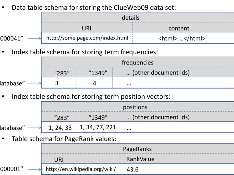
Table schemas in HBase

• Index table schema for storing term frequencies: frequencies

“283” “1349” … (other document ids)

“database” 3 4 …

• Index table schema for storing term position vectors: positions

“283” “1349” … (other document ids) “database” 1, 24, 33 1, 34, 77, 221 …

• Data table schema for storing the ClueWeb09 data set: details

URI content

“20000041” http://some.page.com/index.html _{<html> …</html>}

• Table schema for PageRank values:

PageRanks

URI RankValue

(33)

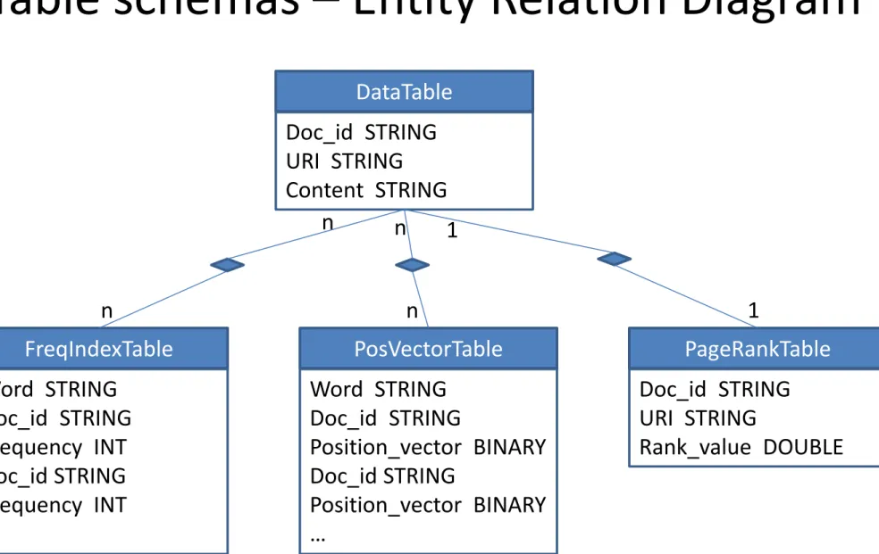
Table schemas – Entity Relation Diagram

DataTable Doc_id STRING URI STRING Content STRING FreqIndexTable Word STRING Doc_id STRING Frequency INT Doc_id STRING Frequency INT … PosVectorTable Word STRING Doc_id STRING Position_vector BINARY Doc_id STRING Position_vector BINARY … PageRankTable Doc_id STRING URI STRING Rank_value DOUBLE n n n n 1 1

(34)

System Architecture

Dynamic HBase deployment Data Loading (MapReduce) Index Building (MapReduce) Term-pair Frequency Counting (MapReduce) Performance Evaluation (MapReduce)

LC-IR Synonym Mining Analysis (MapReduce) CW09DataTable CW09PosVecTable CW09PairFreqTable CW09FreqTable PageRankTable Web Search Interface

(35)

LC-IR Synonym Mining

• Mining synonyms from large document sets based on words’

co-appearances

• Steps for completing LC-IR synonym mining in HBase:

1. Scan the data table and generate a “pair count” table for

word-pairs;

2. Scan the “pair count” table and calculate similarities,

looking up single word hits in the index table;

(36)

Sample Results

- 100 documents indexed, 8499 unique terms

- 3793 (45%) terms appear only once in all documents - Most frequent word: “you”

(37)

Sample Results

• Preliminary performance evaluation

- 6 distributed clients started, each reading 60000 random rows - average speed: 2647 rows/s

• Example synonyms mined (among 16516 documents): - chiropodists podiatrists (0.125, doctors for foot disease) - desflurane isoflurane (0.111, narcotic)

- dynein kinesin (0.111, same type of protein)

- menba monpa (0.125, a nation/race of Chinese people living in Tibet)

(38)

Sample Results

• Original data table size: 29GB (2,594,536 documents)

• Index table size: 8,557,702 rows (one row for each indexed term)

• Largest row: 2,580,938 cell values, 162MB uncompressed size

• At most 1000 cell values are read from each row in this test

• Aggregate read performance increases as number of concurrent clients increases

(39)

Sample Results

Number of nodes Number of mappers Index building time (seconds)

8 32 18590

12 37 (15.6% increase) 16142 (15.2% improvement) 16 47 (46.9% increase) 13480 (37.9% improvement)

• Original data table size: 29GB (2,594,536 documents)

• 6 computing slots on each node

• HBase overhead: data transmission to region servers, cell value sorting based on keys, gzip compression/decompression

• Number of mappers not doubled when number of nodes doubled – because of small table size

• Increase in index building performance is close to increase in number of mappers

(40)

Practical Problems and experiences

• Hadoop and HBase configuration

- Lack of “append” support in some versions of Hadoop: missing data, various errors in HBase and HDFS.

- Low data locality in HBase MapReduce: “c046.cm.cluster” for Task Tracker vs. “c046.cm.cluster.” for Region Server.

- Clock not synchronized error: clock not synched with NTP on some nodes.

• Optimizations in the synonym mining programs

- Addition of a word count table with bloom filter. - Local combiners for word pair counter.

(41)

Low data locality in MapReduce over HBase

• Data splits assigned to mappers by regions (one mapper per region in most cases)

• Mapper deployment based on mapper-region server locality

• Problem: region data blocks not necessarily local to region servers

• Data locality gets even worse after region splits or region server failures Hadoop head node

Job Tracker

Data node Data node

… Task Tracker 2 Region Server 2 Task Tracker 1 Region Server 1 Mapper 1 Mapper 2 a b c c _… d a b _…