NCO Tracking for Singular Control
Problems using Neighboring Extremals
?
S´ebastien Gros∗ Benoˆıt Chachuat∗ Dominique Bonvin∗
∗
Laboratoire d’Automatique, ´Ecole Polytechnique F´ed´erale de Lausanne, CH-1015 Lausanne, Switzerland
(e-mail: [email protected]).
Abstract: A powerful approach for dynamic optimization in the presence of uncertainty is to incorporate measurements into the optimization framework so as to track the necessary conditions of optimality (NCO), the so-called NCO-tracking approach. For nonsingular control problems, this can be done by tracking active constraints along boundary arcs, and using neighboring-extremal (NE) control along interior arcs to force the first-order variation of the NCO to zero. In this paper, an extension of NE control to singular control problems is proposed. The idea is to design NE controllers from successive time differentiations of the first-order variation of the NCO. Based on these results, a NCO-tracking controller that is easily tractable from a real-time optimization perspective is proposed, whose application guarantees that the first-order variation of the NCO converges to zero exponentially. The performance of this NCO-tracking controller is illustrated via the case study of a steered car, a 5th-order two-input dynamical system.
1. INTRODUCTION
Optimization in the process industry has received a lot of attention in recent years because, in the face of growing competition, it represents a natural choice for reducing production costs, improving product quality, and meeting safety requirements and environmental regulations. Tradi-tionally, the optimal operating conditions are determined based on a model of the process. However, the resulting process operation can be highly sensitive to uncertainty such as model mismatch and process disturbances. This generally gives rise to suboptimal process operation or, worse, infeasible operation, which of course is not tolerable in most industrial applications.
A natural approach to combat uncertainty and avoid con-servatism consists in incorporating measurements in the optimization framework. In particular, the NCO-tracking methodology (Srinivasan and Bonvin, 2007) converts a dynamic optimization problem with both path and ter-minal constraints into a feedback control problem. In this approach, near-optimal process operation is enforced by tracking appropriate references, namely the necessary conditions of optimality (NCO). The idea behind NCO tracking is to take advantage of the structure of an optimal control solution, which is usually made of a succession of arcs. For those arcs along which path constraints are active, part of the optimal inputs are obtained by enforcing the corresponding constraints. The remaining part of the optimal inputs is determined by the intrinsic compromises present in the system. In this latter case, the Pontrya-gin Maximum Principle (PMP) (PontryaPontrya-gin et al., 1964) shows that tracking the NCO consists in forcing a sensitiv-ity term to zero. However, this is much more involved than ? This material is based upon work supported by the Swiss National Science Foundation under grant 200020-101783.
constraints tracking in the sense that the corresponding sensitivity terms depend on the adjoint variables, which are typically unknown and cannot be measured. For non-linear dynamical systems, a first-order approximation of these sensitivity terms can be obtained upon application of the theory of neighboring extremals (NE) (Bryson and Ho, 1975). In other words, NE control forces the first-order variation of the NCO to zero, and thus offers much promise in the context of NCO tracking.
However, an inherent limitation of standard NE control lies in the fact that the control problem must be nonsin-gular, otherwise the control law calls for the inversion of a singular matrix. In a previous work, Gros et al. (2004) proposed to design NE controllers for single-input, singular control problems from successive time differentiations of the first-order variation of the NCO. The main contribu-tion of the present paper is to generalize these ideas to the multiple-input case. Most of the complications stem from the fact that an optimal arc for a multiple-input system may have different orders of singularity with respect to the control variables (Robbins, 1967). Based on these new developments, a NCO-tracking controller that is easily implementable and tractable from a real-time optimization perspective is proposed.
The paper is organized as follows. The problem formu-lation is presented in Section 2. NE control for singular problems is characterized in Section 3, and a multiple-input NCO-tracking controller is devised in Section 4. These new developments are illustrated via the case study of a steered car in Section 5. Finally, Section 6 concludes the paper.
2. PROBLEM FORMULATION
Consider the following dynamic optimization problem with input bounds: minJ[u] := Φ(x(tf)) + Z tf 0 L(x(t),u(t),θ) dt (1) s.t. x˙(t) =F(x(t),u(t),θ); x(0) =x0 (2) uL ≤u(t)≤uU, (3)
where t stands for the time (independent) variable, tf the fixed final time, u : [0, tf] → Rnu the control vector function, x : [0, tf] → Rnx the state vector function with initial state x0, θ ∈ Rnθ the vector of uncertain time-invariant parameters,Fthe system dynamics,J the scalar cost functional to be minimized, Φ the terminal cost function, andLthe integral cost function. We shall assume that all functions appearing in (1)–(3) are sufficiently often continuously differentiable with respect to their arguments.
The first- and second-order necessary conditions of opti-mality for the problem (1)–(3) are given by:
Hu =Lu+FTuλ−µ
L+
µU =0 (4)
Huu positive semi-definite,
where the Hamiltonian function H is defined as
H(x,u,θ,λ,µL,µU) :=L(x,u,θ) +F(x,u,θ)Tλ
+µLT(uL−u) +µUT(u−uU),
λ: [0, tf]→Rnx denotes the adjoint vector function given by
˙
λ= −Hx=−FTxλ−Lx; λ(tf) = Φx(x(tf)), and µL,µU : [0, t
f]→Rnu are Lagrange multiplier vector functions satisfying
µLT(uL−u) =0; µL≥0
µUT(u−uU) =0; µU ≥0.
Given the nominal parameter values ¯θ, we shall assume that a unique optimal control u∗
(t), 0 ≤t ≤tf, exists in the class of piecewise-continuous vector functions for the optimization problem (1)–(3). We shall call the piece of an optimal trajectory that does not intersect the boundary an interior arc; if at least one constraint is active, we call that piece of trajectory aboundary arc. Observe that
µL(t) = µU(t) = 0 along an interior arc, while there is some i ∈ {1, . . . , nu} such that µLi(t) 6= 0 or µUi (t) 6= 0 along a boundary arc.
In optimal control theory, singular control problems are those for which a straightforward application of the fore-going NCO fails to provide adequate tests for singling out optimal control values (Bell and Jacobson, 1975). In other words, the matrix Huu is singular. To determine
optimal control values along singular arcs, one usually exploits the identical vanishing of Hu and its successive
time derivatives ˙Hu,H¨u, . . .
3. CHARACTERIZATION OF NE CONTROL Any slight change ηδx0 in the initial state or ηδθ in the model parameters modifies the optimal control trajectory
u∗
(t), 0 ≤ t ≤ tf, and requires that it be recalculated.
Clearly, calculating a perturbed optimal control is a time-consuming task, hardly compatible with the objective of real-time optimization. A more tractable way of obtaining a perturbed optimal control trajectory is to consider the first-order approximation
u(t;η) =u∗
(t) +ηδu(t) +o(η),
and then use the theory of neighboring extremals for calculating the correction δu in such a way that the first-order variation of the NCO be equal to zero upon application of the controlu∗
(t) +ηδu(t). Let (u∗(t),x∗(t),
λ∗
(t)), 0 ≤t ≤ tf, be an optimal triple for the optimal control problem (1)–(3) corresponding to the nominal parameter values ¯θ. Along each arc composing
u∗
, a control variableu∗
i(t) may either:
• belong to the interior of the control region uL i <
u∗
i(t) < uUi , in which case a neighboring-extremal solution is such thatδµL
i(t) =δµUi (t) = 0, andδui(t) is obtained from the first variation of (4) as
δHui=H ∗ uixδx+F ∗T uiδλ+H ∗ uuiδui+H ∗ uiθδθ= 0; • or be at one of its boundariesuL
i oru U
i , in which case a NE control is simply given byδui(t) = 0.
Thesenuconditions can be written collectively in the form
δL:=A0δλ+B0δx+C0δu+D0δθ=0, (5) where A0(t),B0(t)∈ Rnu×nx, C0(t) ∈ Rnu×nu, D0(t) ∈ Rnu×nθ, and δx˙ =F∗ xδx+F ∗ uδu+F ∗ θδθ δλ˙ = −F∗T x δλ−H ∗ xxδx−H ∗ xuδu−H ∗ xθδθ δx(0) =δx0, δλ(tf) = Φ∗xxδx(tf).
IfC0 has full rank, a NE control law is readily obtained from (5) as
δu= −C−1
0 [A0δλ+B0δx+D0δθ],
which corresponds to the standard NE control law in the case where no input constraint is active (Bryson and Ho, 1975).
On the other hand, ifC0 is singular and of constant rank (nu−r0), singular value decomposition (SVD) ofC0 gives
(Uns0 Us0) Σ0 0r0×r0 Vns0 T Vs0T :=C0,
whereΣ0is a diagonal, positive-definite matrix, andU0:= (Uns0 Us0), V0 := (V0ns Vs0) are orthogonal matrices. The input variations δu(t) can then be partitioned into nonsingularδuns
0 (t) and singularδus0(t) subparts of dimen-sion (nu−r0) andr0, respectively,
δuns0 (t) =Vns0 T
(t)δu(t), δus0(t) =Vs0 T
(t)δu(t).
Using this partition, the conditions (5) can be split into
0=Uns0 TδL=Uns0 T(A0δλ+B0δx+D0δθ) +Σ0δuns0
0=Us0TδL=Us0T(A0δλ+B0δx+D0δθ).
MatrixΣ0being invertible, the former (nu−r0) conditions provide an explicit expression for the nonsingular control variationsδuns
0 as
δuns0 = −Σ
−1
0 Uns0 T(A0δλ+B0δx+D0δθ). The remainingr0 singular control variationsδus0 are de-termined from the latter r0 conditions. Introducing the
new variables δ`0 := Us0TδL ∈ Rr0, and differentiating
δ`0 twice with respect to time leads to 2r0 additional conditions of the form
0=δ`˙0=A1δλ+B1δx+D1δθ
0=δ¨`0=A2δλ+B2δx+C2δus0+D2δθ, (6) with A1,B1,A2,B2 ∈ Rr0×nx, D1,D2 ∈ Rr0×nθ, and
C2∈Rr0×r0.
At this point, we have either one of two cases:
• IfC2 has full rank, the singular NE controlδus0(t) is obtained from (6) as
δus
0= −C
−1
2 (A2δλ+B2δx+D2δθ). The NE control law is then obtained by piecing singular and nonsingular control variations together as δu= −Vns0 Σ−1 0 Uns0 T (A0δλ+B0δx+D0δθ) −Vs0C−1 2 (A2δλ+B2δx+D2δθ) ;
• If C2 is singular and of constant rank (r0 −r2), one uses SVD ofC2 to further partition the singular control variations as δuns
2 :=Vns2 Tδus0 ∈Rr0−r2 and
δus
2 := V2sTδus0 ∈ Rr2. Then, introducing the new variables δ`2 := Us2Tδ¨`0 ∈ Rr2, one can proceed as before by differentiatingδ`2twice, and the procedure continues in an obvious manner.
By continuing the recursion outlined previously, that is
δ`2k:=Us2k Tδ¨
`2k−2∈Rr2k; δ`0:=Us0TδL, (7) one obtains the following set of 3r2k−2 conditions that must hold along a singular arc:
0=δ`2k−2=Us2k−2 T(A 2k−2δλ+B2k−2δx+D2k−2δθ) 0=δ`˙2k−2=A2k−1δλ+B2k−1δx+D2k−1δθ 0=δ¨`2k−2=A2kδλ+B2kδx+C2kδus2k−2+D2kδθ, whereA2k−1,B2k−1,A2k,B2k∈Rr2k−2×nx,D2k−1,D2k ∈ Rr2k−2×nθ,C
2k ∈Rr2k−2×r2k−2 are defined recursively as
A2k−1= ˙UsT2k−2A2k−2 (8) +UsT2k−2 ˙ A2k−2−A2k−2F ∗T x B2k−1= ˙UsT2k−2B2k−2 (9) +UsT2k−2 ˙ B2k−2+B2k−2F ∗ x−A2k−2H ∗ xx D2k−1= ˙U sT 2k−2D2k−2 (10) +UsT2k−2 ˙ D2k−2+B2k−2F∗θ−A2k−2Hx∗θ A2k = ˙A2k−1−A2k−1F∗xT (11) −(B2k−1F ∗ u−A2k−1H ∗ xu) × k−1 X i=0 i−1 Y j=0 Vs2j Vns2iΣ −1 2i U ns 2i T A2i B2k= ˙B2k−1+B2k−1F∗x−A2k−1Hxx∗ (12) −(B2k−1F ∗ u−A2k−1H ∗ xu) × k−1 X i=0 i−1 Y j=0 Vs2j Vns2iΣ −1 2i U ns 2i T B2i C2k = (B2k−1F ∗ u−A2k−1H ∗ xu) k−1 Y j=0 Vs2j (13) D2k = ˙D2k−1+B2k−1F ∗ θ−A2k−1Hx∗θ (14) −(B2k−1F ∗ u−A2k−1H ∗ xu) × k−1 X i=0 i−1 Y j=0 V2sj Vns2iΣ−1 2i U ns 2i T D2i ,
and the matrices Uns2k, Us2k, V2nsk and Vs2k are obtained from SVD ofC2k as (Uns2k Us2k) Σ2k 0r2k×r2k Vns2kT Vs2kT :=C2k. (15)
It is assumed throughout that the rank (r2k−2−r2k) of the matrixC2k is constant along the singular arc for each
k= 0,1, . . .
The procedure is stopped afterpiterations, wherepstands for the smallest value ofksuch thatC2pis nonsingular. A finite value is assumed forpin this work, i.e. the control problem is not degenerate. Then, the control variation
δu(t) is obtained by piecing nonsingular and singular control variations together,
δu= p−1 X k=0 k−1 Y i=0 Vs2i ! V2nskδuns2k+ p−1 Y i=0 Vs2i ! δus2p−2, (16) where the control variations δuns
0 (t), . . . , δuns2p−2(t), and
δus
2p−2(t) are obtained from the conditions δ¨`2k−2 = 0
as δuns2k = −Σ −1 2kU ns 2k T (A2kδλ+B2kδx+D2kδθ) δus 2p−2= −C −1 2p (A2pδλ+B2pδx+D2pδθ). 4. DESIGN OF NCO-TRACKING CONTROLLERS In general, the junction times between the various arcs constituting the optimal solution u∗
(t), 0 ≤ t ≤ tf, vary when initial conditions or model parameters are perturbed. For many control problems, however, these variations remain small and can be ignored without much effect on system performance. This is the case, e.g., when the nominal solution is dominated by a small number of (possibly singular) arcs. We shall see in this section how simple NCO-tracking controllers can be devised for such problems by fixing the junction times to their nominal values. The resulting controllers are advantageous from a practical viewpoint because the state feedback law comes as a closed-form expression, i.e. it does not necessitate time-consuming on-line computations (such as the on-line solution of a TPBVP).
By construction, applying the feedback law (16) guaran-tees that the conditions Uns0 TδL = 0, U2nskTδ¨`2k−2 =0,
k = 1, . . . , p−1, and δ¨`2p−2 = 0 are satisfied along a singular arc. Yet, the remaining conditions Us
0 T δL =0, Us 2k Tδ¨`
2k−2 = 0 and δ`˙2k−2 = 0, k = 1, . . . , p, are not
enforced by (16) and may be violated when the junction times are fixed; in particular, this leads to a violation of the first-order variation of the NCO,δL=0.
A way of enforcing this latter condition is to modify the recursion (7) as
δ`2k:=Us2k TT
2k−2δ`2k−2; δ`0:=Us0TδL, where the operatorT2k−2 is given by
T2k−2:= d2 dt2 +γ 1 2k−2 d dt+γ 0 2k−2, (17) and γ0
2k−2, γ21k−2 ∈ R are constant gain coefficients. By finite induction onk= 1, . . . , p−1, it can be shown that this modification leads to the following expressions:
δ`2k=Us2k T A¯ 2kδλ+ ¯B2kδx+ ¯D2kδθ δ`˙2k=A2k+1δλ+B2k+1δx+D2k+1δθ δ¨`2k=A2k+2δλ+B2k+2δx+C2k+2δus2k+D2k+2δθ, where: ¯ A2k=A2k+γ21k−2A2k−1+γ 0 2k−2Us2k−2 TA 2k−2 ¯ B2k=B2k+γ21k−2B2k−1+γ 0 2k−2U s 2k−2 T B2k−2 ¯ D2k=D2k+γ21k−2D2k−1+γ20k−2Us2k−2 TD 2k−2 ¯ A0=A0, B¯0=B0, D¯0=D0.
The matrices A2k+1,B2k+1,D2k+1 are calculated as in (8)–(10);A2k,B2k,C2k,D2kare calculated as in (11)–(14) except that A2i, B2i, and D2i are now replaced by ¯A2i,
¯
B2i, and ¯D2i; the matrices Uns2k, Us2k, Vns2k and Vs2k are obtained from SVD ofC2k as in (15).
Observe that the expression ofδ¨`2k−2being the same as in Section 3, the expression of the new feedback is identical to (16), with the modified matrices ¯A2k,B¯2k,D¯2k. This feedback law can be rewritten in more compact form
δu(t) =−C(t) [A(t)δλ(t) +B(t)δx(t) +D(t)δθ], (18)
with the matrices A,B ∈ R(r0+···+r2p)×nx, D ∈
R(r0+···+r2p)×np, and C∈Rnu×(r0+···+r2p) given by:
A:= ¯ A0 ¯ A2 .. . ¯ A2p , B:= ¯ B0 ¯ B2 .. . ¯ B2p , D:= ¯ D0 ¯ D2 .. . ¯ D2p , C:= · · · k−1 Y i=0 Vs2iVns2kΣ−1 2kU ns 2k T · · · p−1 Y i=0 V2si C−1 2p ! .
The following theorem shows that, under mild assump-tions, the modified NE feedback law (18) drives the first-order variation of the NCO to zero, in response to vari-ations in both the initial condition δx0 and the model parametersδθ.
Theorem 1. Let Γ2k ∈R2×2be defined as Γ2k:= 0 1 −γ0 2k −γ12k .
If Γ2k is Hurwitz for eachk = 0, . . . , p−1, then the first variationδLof the NCO converges to zero exponentially
upon application of the feedback law (18).
Proof. See Gros (2007) for a proof. The gain coefficients γ0
2k, γ21k, 0 ≤ k < p, determine the rate of convergence ofδLand must be selected carefully.
While too small values may not allow to reject the per-turbations sufficiently rapidly relative to the time horizon [0, tf], large values may lead to excessive corrections that invalidate the linear approximation and make the feedback highly sensitive to measurement noise. As a possible exten-sion, one may consider gain matrices Γ0
2k,Γ12k ∈R r2k×r2k
instead of scalar gain coefficients. It can be shown that the result in Theorem 1 still holds, provided that the (2r2k×2r2k) matrix 0r2k×r2k Ir2k×r2k −Γ02k −Γ12k is Hurwitz, for eachk= 0, . . . , p−1.
Finally, an explicit feedback law is obtained from (18) based on the backward sweep method (Bryson and Ho, 1975): δu(t) = −Kx(t)δx(t)−Kθ(t)δθ (19) Kx(t) =C(t) [A(t)Sx(t) +B(t)] (20) Kθ(t) =C(t) [A(t)Sθ(t) +D(t)] (21) ˙ Sx(t) = −H ∗ xx−Sx(t)F ∗ x−F ∗T x Sx(t) (22) + [H∗ xu+Sx(t)F ∗ u]Kx(t); Sx(tf) = Φ∗xx ˙ Sθ(t) = −H∗ xθ−Sx(t)F ∗ θ−F ∗T x Sθ(t) (23) + [H∗ xu+Sx(t)F ∗ u]Kθ(t); Sθ(tf) =0. Because this control law drives the first-variation of the NCO to zero, (19)–(23) can be seen as a NCO-tracking controller. Note that, for the integration of the sweep matrices Sx, Sθ to remain stable, the gain coefficients
γ0
2k, γ21k, 0≤k < p, must not be too large. A tradeoff must therefore be sought, which is clearly problem dependent.
5. CASE STUDY1
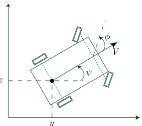
To illustrate the design and performance of NCO-tracking controllers for singular control problems, a steered car with inertia and friction is considered (see Fig. 1). A model describing the motion of the car is as follows
˙ y=V cosψ; y(0) =y0 (24) ˙ z=V sinψ; z(0) =z0 (25) ˙ V =u1−µV; V(0) = 0 (26) ˙ ψ=V tanφ; ψ(0) = 0 (27) ˙ φ=u2; φ(0) = 0, (28)
where y and z denote the Cartesian coordinates of the car [m], V its velocity [m/s], ψ its heading angle [rad],
φ the orientation of its driving wheels [rad], and µ is a friction parameter [1/s]. The control variableu1represents the motor force divided by the mass of the car [N/kg], and the control variable u2 stands for the rate of change of the orientation of the driving wheels [rad/s]. A quadrature variable,E, representing the cumulated energy consump-tion per unit mass [J/kg] is added to the model:
˙
E=u1V; E(0) = 0. (29)
Note that ˙Emay be negative whenu1opposesV, meaning that the car has the ability to recover energy from braking (regenerative braking system). The numerical values for the parameters, initial conditions, and input bounds are given in Tab. 1.
The optimization problem consists in minimizing the en-ergy needed to bring the car to a neighborhood of the origin (0,0) at a fixed final tf, while respecting input bounds:
1 Note to the reviewers.As far as possible, the case study of a
multiple-input chemical process will be included in the final version of the paper.
PSfrag replacements z y ψ φ V
Fig. 1. Steered car with indication of the state variables. minimize : J[u] :=y(tf)2+z(tf)2+E(tf) (30) subject to : model equations (24)−(29) (31)
uL
1 ≤u1(t)≤uU1 (32)
uL2 ≤u2(t)≤uU2. (33)
5.1 Design of the NCO-Tracking Controller
The design of the NCO-tracking controller starts with the computation of the nominal optimal control. Possible values that can be taken by the inputs u1(t) and u2(t) along an optimal solution are determined upon application of Pontryagin’s Maximum Principle:
• the interior arcs for the inputu1are singular of degree
p1 = 1, and the values taken by u∗1(t) along an optimal solution are restricted to {uL
1, uU1, µV(t)− λ4(t)
2µ(cosφ(t))2uL2, µV(t)−
λ4(t)
2µ(cosφ(t))2uU2, µV(t)};
• the interior arcs for the inputu2are singular of degree
p2= 2, andu∗2(t) can only take on discrete values in {uL
2, uU2,0}along an optimal solution.
To get an idea of the optimal sequence of arcs, a numerical solution to the problem (30)–(33) is computed using the control vector parameterization (CVP) approach. The optimal solution appears to be constituted of 6 principal arcs, separated by 5 switching times t∗
k, k = 1, . . . ,5 (Tab. 2).
Based on this arc sequence, a NCO-tracking controller is designed following the procedure described in Sections 3 and 4. In this controller, the junction times are fixed to
Table 1. Model parameters, initial conditions, and input bounds.
µ 0.1 1/s uL 1 −1 N/kg y0 −4 m u U 1 1 N/kg z0 4 m uL 2 −1 N/kg tf 8 s uU 2 1 rad/s Table 2. Nominal arc sequence.
Arc u1 u2 1 uU 1 u L 2 2 using1 (t) u L 2 3 using1 (t) uU 2 4 using1 (t) uL 2 5 using1 (t) u sing 2 (t) 6 uL 1 u sing 2 (t)
Table 3. NCO-tracking controller. Arc Controller for
u1 u2 1 none none 2 NE controller 1 3 4 5 NE controller 2 6 none NE controller 3 their nominal values t∗
k, k = 1, . . . ,5, and the corrective actions taken along each arc are those indicated in Tab. 3. The design of the three NE controllers is based on (19)– (23) and requires the computation of the time-varying matrices A, B, C and D. Although the SVD procedure
described in Section 3 gives constant singular and nonsin-gular directions in this example (i.e.,Uns2k,Us2k,Vns2k,Vs2k
are constant matrices), performing those calculations by hand is both fastidious and prone to errors. Fortunately, the theory lends itself naturally to automation, e.g., with the symbolic toolbox ofMatlabr.
• In the NE controller 1, the recursion starts with the conditions 0=δL(t) = δλ3(t) +δV(t) δu2(t) , t∗ 1< t≤t ∗ 4. The matrix C0 has rank nu−r0 = 1, and 2 time differentiations are required to devise the controller, i.e.p= 1.
• In the NE controller 2, the recursion starts with the conditions 0=δL(t) = δλ3(t) +δV(t) δλ5(t) , t∗ 4< t≤t ∗ 5. The matrix C0 has ranknu−r0 = 0. The compu-tations giver2 = 1 after 2 rounds of differentiations, and a total of 4 successive differentiations is necessary to design the controller, i.e.p= 2.
• Finally, the recursion for the NE controller 3 starts with the conditions
0=δL(t) = δu1(t) δλ5(t) , t∗ 5 < t≤tf. The matrix C0 has ranknu−r0 = 1. The compu-tations giver2 = 1 after 2 rounds of differentiations, and a total of 4 successive differentiations is necessary to design the controller, i.e.p= 2.
The gain coefficients in the NE controller 1 are taken as γ0
0 = s1s2 and γ01 = −s1s2, so that the differential operatorT0 given in (17) has stable poles at s1 = −0.2 and s2=−2. On the other hand, the gain coefficients in the NE controllers 2 and 3 are taken as γ0
0 = γ20 = s2 and γ1
0 = γ21 = −2s, so that T0 and T2 both have stable poles at s = −1. Decreasing the poles leads to more aggressive NE controllers in the sense that the inputs are more likely to saturate at their upper or lower bounds. Generally, decreasing the poles also has an adverse effect on the stability of the backward sweep integration.
5.2 Performance of the NCO-Tracking Controller
To assess the performance of the proposed control ap-proach, a scenario is considered where the initial conditions are perturbed as ψ(0) = −0.175 [rad] and V(0) = 0.5
Table 4. Compared performance of various control strategies.
Control Strategy J
Optimal Solution (Ideal) 0.7015 Open-Loop Nominal Solution 10.084
NCO Tracking 0.8034
NCO Tracking with NE Control on Arc 5 only 1.1005 [m/s], and the friction parameter is perturbed asµ= 0.2 [1/s]. Note that these are substantial perturbations of the nominal operating conditions.
The NCO-tracking controller is compared to:
(1) the optimal solution to the perturbed problem, as-suming known perturbations;
(2) the optimal solution to the nominal problem, applied open loop;
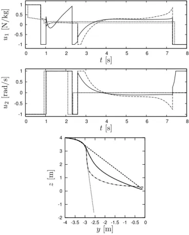
(3) a simplified NCO-tracking controller implementing a two-input NE controller on Arc 5 and applying the nominal control open loop along the remaining arcs. The input and response trajectories for the various control strategies are shown in Fig. 2. Moreover, the cost obtained with each strategy is reported in Tab. 4. Note that ap-plying the nominal input open loop leads to poor perfor-mance. On the other hand, the proposed NCO-tracking controller is able to recover most of the performance loss compared to the optimal strategy (which assumes that the perturbed initial conditions are known). Interestingly enough, most of the performance loss is also recovered upon application of a two-input NE controller along Arc 5 only (NE controller 2), while leaving the remaining arcs uncontrolled. This comparison clearly illustrates the cen-tral role played by the NE controller 2 in the NCO-tracking scheme.
6. CONCLUSIONS AND FUTURE WORK Many practical problems of interest exhibit solutions that contain singular arcs, e.g., in rocket and air vehicle flight or chemical plant operation. Strong incentives therefore exist to operate these processes in the most efficient possible manner, despite the presence of uncertainty. In this paper, an extension of the theory of neighboring extremals to address singular optimal control problem has been proposed for multiple-input system. Moreover, to make these results tractable from a real-time optimization perspective, an explicit NCO-tracking controller has been devised, which guarantees that, under mild assumptions, the first-order variation of the NCO converge to zero exponentially. These results have been illustrated by the case study of a steered car. It is found that the NCO-tracking controller not only allows to recover most of the optimality loss induced by large perturbations of the initial conditions, but it also shows excellent performance in the presence of substantial parameter uncertainty.
Despite the apparent complexity of designing NE con-trollers for singular control problems, it should be empha-sized that most of this complexity is dealt with off-line. In particular, on-line calculations are limited to the imple-mentation of a simple state-feedback law. This approach is therefore well suited to control fast dynamical systems. An important limitation of the approach lies in the fact that
full state measurement is required in the NE feedback law. The design of NE controllers based on output feedback will be the topic of future research. Future developments will also aim at handling those optimal control problems for which fixing the junction leads to large performance loss.
REFERENCES
D. J. Bell and D. H. Jacobson. Singular Optimal Control Problems. Academic Press, 1975.
A. E. Bryson and Y. C. Ho. Applied Optimal Control. Hemisphere, Washington DC, 1975.
S. Gros. Neighboring Extremals in Optimization and Control. PhD thesis, ´Ecole Polytechnique F´ed´erale de Lausanne, Switzerland, 2007.
S. Gros, B. Srinivasan, and D. Bonvin. Neighboring extremal controllers for singular problems. InProc. 2004 American Control Conference, pages 34–39, Boston, MA, 2004.
L. S. Pontryagin, V. G. Boltyanskii, R. V. Gamkrelidze, and E. F. Mishchenko. The Mathematical Theory of Optimal Processes. Pergamon Press, New York, 1964. H. M. Robbins. A generalized legendre-clebsch condition
for the singular cases of optimal control. IBM J Res Dev, 11(4):361–372, 1967.
B. Srinivasan and D. Bonvin. Real-time optimization of batch processes via tracking of necessary conditions of optimality. Ind Eng Chem Res, 46(2):492–504, 2007.
-1 -0.5 0 0.5 1 0 1 2 3 4 5 6 7 8 -1 -0.5 0 0.5 1 0 1 2 3 4 5 6 7 8 PSfrag replacements t[s] t[s] u1 [N/kg] u2 [rad/s] y[m] z[m] -2 -1 0 1 2 3 4 -4 -3.5 -3 -2.5 -2 -1.5 -1 -0.5 0 PSfrag replacements t[s] u1 [N/kg] u2 [rad/s] y [m] z [m]
Fig. 2. Comparison of the input and state trajectories obtained with different control strategies. Dashed line: optimal solution to the perturbed problem; solid line: NCO tracking; dash-dotted line: NCO tracking on Arc 5 only; dotted line: optimal nominal solution applied open loop.