Supervised learning based on temporal coding in
spiking neural networks
Hesham Mostafa Institute of Neuroinformatics University of Zurich and ETH Zurich
Abstract
Gradient descent training techniques are remarkably successful in training analog-valued artificial neural networks (ANNs). Such training techniques, however, do not transfer easily to spiking networks due to the spike generation hard non-linearity and the discrete nature of spike communication. We show that in a feedforward spiking network that uses a temporal coding scheme where information is encoded in spike times instead of spike rates, the network input-output relation is differentiable almost everywhere. Moreover, this relation is locally linear after a transformation of variables. Methods for training ANNs thus carry directly to the training of such spiking networks as we show when training on the permutation invariant MNIST task. In contrast to rate-based spiking networks that are often used to approximate the behavior of ANNs, the networks we present spike much more sparsely and their behavior can not be directly approximated by conventional ANNs. Our results highlight a new approach for controlling the behavior of spiking networks with realistic temporal dynamics, opening up the potential for using these networks to process spike patterns with complex temporal information.
1
Introduction
Artificial neural networks (ANNs) are enjoying great success as a means of learning complex non-linear transformations by example [1]. The idea of a distributed network of simple neuron elements that adaptively adjusts its connection weights based on training examples is partially inspired by the operation of biological spiking networks [2]. ANNs, however, are fundamentally different from spiking networks. Unlike ANN neurons that are analog-valued, spiking neurons communicate using all-or-nothing discrete spikes. A spike triggers a trace of synaptic current in the target neuron. The target neuron integrates synaptic current over time until a threshold is reached, and then emits a spike and resets. Spiking networks are dynamical systems in which time plays a crucial role, while time is abstracted away in conventional feedforward ANNs.
While there exist well-developed techniques for training feedforward ANNs (mainly based on gradient descent), there is no general technique for training feedforward spiking neural networks. An approach that bears some similarities to ours is the SpikeProp algorithm [3] that can be used to train spiking networks to produce output spikes at specific times. SpikeProp assumes a connection between two spiking neurons consists of a number of sub-connections, each with a different delay and a trainable weight. We use a more conventional network model that does not depend on combinations of pre-specified delay elements to transform input spike times to output spike times, and instead relies only on simple neural and synaptic dynamics. Many approaches for training spiking networks first train conventional feedforward ANNs and then translate the trained weights to spiking networks developed to approximate the behavior of the original ANNs [4, 5, 6]. The spiking networks obtained using these methods use rate coding where the spiking rate of a neuron encodes an analog quantity corresponding to the analog output of an ANN neuron.
In this paper, we develop a direct training approach that does not try to reduce spiking networks to conventional ANNs. Instead, we relate the time of any spike differentiably to the times of all spikes that had a causal influence on its generation. We can then impose any differentiable cost function on the spike times of the network and minimize this cost function directly through gradient descent. By using spike times as the information-carrying quantities, we avoid having to work with discrete spike counts or spike rates, and instead work with a continuous representation (spike times) that is amenable to gradient descent training. This training approach allows detailed control over the behavior of the network (at the level of single spike times) which would not be possible in training approaches based on rate-coding.
Since we use a temporal spike code, neuron firing can be quite sparse as each spike carries significant information. Compared to rate-based networks, the networks we present can be implemented more efficiently on neuromorphic architectures where power consumption decreases as spike rates are reduced [7, 8, 9]. The behavior of the networks we present deviates quite significantly from that of conventional ANNs. They represent an alternative network paradigm where continuous time is explicitly modeled and used as a coding dimension, but which can still be directly and effectively trained using standard gradient descent methods.
2
Network model
We use non-leaky integrate and fire neurons with exponentially decaying synaptic current kernels. The neuron’s membrane dynamics are described by:
dVmemj (t) dt = X i wji X r κ(t−tri) (1) where Vj
mem is the membrane potential of neuronj. The right hand side of the equation is the
synaptic current.wjiis the weight of the synaptic connection from neuronito neuronjandtri is the
time of therthspike from neuroni.κis the synaptic current kernel given by:
κ(x) = Θ(x)exp(− x τsyn ) where Θ(x) = 1 if x≥0 0 otherwise (2)
Synaptic current thus jumps instantaneously on the arrival of an input spike, then decays exponentially with time constantτsyn. Sinceτsynis the only time constant in the model, we set it to 1 in the rest of
the paper, i.e, normalize all times with respect to it. The neuron spikes when its membrane potential crosses a firing threshold which we set to1, i.e, all synaptic weights are normalized with respect to the firing threshold. The membrane potential is reset to0after a spike. We allow the membrane potential to go below zero if the integral of the synaptic current is negative.
Assume a neuron receivesNspikes at times{t1, .., tN}with weights{w1, .., wN}fromNsource
neurons. Each weight can be positive or negative. Assume the neuron spikes in response at timetout.
By integrating Eq. 1, the membrane potential fort < toutis given by:
Vmem(t) = N X
i=1
Θ(t−ti)wi(1−exp(−(t−ti))) (3)
Assume only a subset of these input spikes with indices inC ⊆ {1, .., N}had arrived beforetout
whereC={i:ti< tout}. It is only these input spikes that influence the time of the output neuron’s
first spike. We call this set of input spikes the causal set of input spikes. The sum of the weights of the causal input spikes has to be larger than 1, otherwise they could not have caused the neuron to fire. From Eq. 3,toutis then implicitly defined as:
1 =X
i∈C
wi(1−exp(−(tout−ti))) (4)
where1is the firing threshold. Hence,
exp(tout) = P i∈C wiexp(ti) P i∈C wi−1 (5)
Spike times always appear exponentiated. Therefore, we do a transformation of variables exp(tx)→zx yielding an expression relating input spike times to the time of the first spike of
the output neuron in the post-transformation domain (which we denote as the z-domain):
zout= P i∈C wizi P i∈C wi−1 (6)
Note that for the neuron to spike in the first place, we must have P i∈C
wi >1, sozout is always
positive (one can show this is the case even if some of the weights are negative). It is also always larger than any element of{zi :i∈C}, i.e, the output spike time is always larger than any input
spike time in the causal set which follows from the definition of the causal set. We can obtain a similar expression relating the time of theLthspike of the output neuron,zL
out, to the input spike
times in the z-domain:
zLout= P i∈CL wizi P i∈CL wi−L (7)
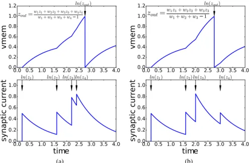
whereCLis the set of indices of the input spikes that arrive before theLthoutput spike. Equation 7 is only valid if the denominator is positive, i.e, there are sufficient input spikes with large enough total positive weight to push the neuron past the firing thresholdLtimes. In the rest of the paper, we consider a neuron’s output value to be the time of its first spike. During training, we use a weight cost term that insures the neuron receives sufficient input to spike as we describe in the next section. The linear relation between input and output spike times in the z-domain is only valid in a local interval. A different linear relation holds when the set of causal input spikes changes. This is illustrated in Fig. 1, where the 4th input spike is part of the causal set in one case but not in the other. From Eq. 6, the effective weight of inputzpin the linear input-output relation in the z-domain is
wp/(P i∈C
wi−1). This effective weight depends on the weights of the spikes in the causal set of
input spikes. As this causal set changes due to the changing spike times from the source neurons, the effective weight of the different input spikes that remain in the causal set changes (as is the case for the first three spikes in Figs. 1a and 1b whose effective weight changes as the causal set changes, even though their actual synaptic weights are the same ). For some input patterns, Some source neurons may spike late causing their spikes to leave the causal set of the output neuron and their effective spike weights to become zero. Other source neurons may spike early and influence the timing of the output neuron’s spike and thus their spikes acquire a non-zero effective weight. The causal set of input spikes is dynamically determined based on the input spike times and their weights. Many early spikes with strong positive weights will cause the output neuron to spike early, negating the effect of later spikes on the output neuron’s first spike time regardless of the weights of these later spikes. The non-linear transformation fromz={z1, .., zN}tozoutimplemented by
the spiking neuron is thus fundamentally different from the static non-linearities used in traditional ANNs where only the aggregate weighted input is considered.
The non-linear transformation implemented by the spiking neuron is continuous in most case, i.e, small perturbation inzwill lead to proportionately small perturbations inzout. This is clear
when the perturbations do not change the set of causal input spikes as the same linear relation continues to hold. Consider, however, the case of an input spike with weightwxthat occurs just
after the output spike at timezx = zout +. A small perturbation pushes this input spike to
timezx = zout −adding it to the causal set. By applying Eq. 6, the perturbed output time is
zoutperturb= ( P i∈C
wizi+wxzx)/(P i∈C
wi+wx−1)whereCis the causal set before the perturbation.
Substituting forzx,z perturb
out −zout =−wx/(P
i∈C
wi+wx−1). The output perturbation is thus
proportional to the input perturbation but this is only the case when P i∈C
wi+wx >1, otherwise
the perturbed input spike with negative weight atzout−would cancel the original output spike at
zout. In summary, the input spike times to output spike time transformation of the spiking neuron is
0.0 0.5 1.0 1.5 2.0 2.5 3.0 3.5 4.0 0.0 0.2 0.4 0.6 0.8 1.0 1.2 vmem zout=w1wz11++ww22z+2+w3w+3zw34+−w14z4 ln(zout) 0.0 0.5 1.0 1.5 2.0 2.5 3.0 3.5 4.0 time 0.0 0.2 0.4 0.6 0.8 1.0 syn aptic curr ent ln(z1) ln(z2)ln(z3)ln(z4) (a) 0.0 0.5 1.0 1.5 2.0 2.5 3.0 3.5 4.0 0.0 0.2 0.4 0.6 0.8 1.0 1.2 vmem zout=ww1z1+w2z2+w3z3 1+w2+w3−1 ln(zout) 0.0 0.5 1.0 1.5 2.0 2.5 3.0 3.5 4.0 time 0.0 0.2 0.4 0.6 0.8 1.0 syn aptic curr ent ln(z1) ln(z2)ln(z3) ln(z4) (b)
Figure 1: Changes in the causal input set modify the linear input-output spike times relation. Plots show the synaptic current and the membrane potential of a neuron in two situations: in a, the neuron receives 4 spikes with weights{w1, w2, w3, w4}at the times indicated by the black arrows in the
bottom plot. This causes the neuron to spike at timetout=ln(zout); in b, input spike times change
causing the neuron to spike before the fourth input spike arrives. This changes the linear z-domain input-output relation of the neuron compared to a.
3
Training
We consider feedforward neural networks where the neural and synaptic dynamics are described by Eqs. 1 and 2. The neurons are arranged in a layer-wise manner. Neurons in one layer project in an all-to-all fashion to neurons in the subsequent layer. A neuron’s output is the time of its first spike and we work exclusively in the z-domain. The forward pass is described in Algorithm 1. All indices are 1-based, vectors are in boldface, and theithentry of a vectoraisa[i]. At each layer, the
causal set for each neuron is obtained from theget causal setfunction. The neuron output is then evaluated according to Eq. 6. Theget causal setfunction is shown in algorithm 2. It first sorts the input spike times, and then considers increasingly larger sets of the early input spikes until it finds a set of input spikes that causes the neuron to spike. The output neuron must spike at a time that is less than the time of any input spike not in the causal set, otherwise the causal set is incomplete. If no such set exists, i.e, the output neuron does not spike in response to the input spikes,get causal set returns the empty setΦand the neuron’s output spike time is set to infinity (maximum positive value in implementation).
From Eq. 6, the derivatives of a neuron’s first spike time with respect to synaptic weights and input spike times are given by:
dzout dwp = zp−zout P i∈C wi−1 if p∈C 0 otherwise (8) dzout dzp = wp P i∈C wi−1 if p∈C 0 otherwise (9)
Unlike the spiking neuron’s input-output relation which can still be continuous at points where the causal set changes, the derivative of the neuron’s output with respect to inputs and weights given by Eqs. 8 and 9 is discontinuous at such points. This is not a severe problem for gradient descent methods. Indeed, many feedforward ANNs use activation functions with a discontinuous first derivative such as rectified linear units (ReLUs) [10] while still being effectively trainable.
A differentiable cost function can be imposed on the spike times generated anywhere in the network. The gradient of the cost function with respect to the weights in lower layers can be evaluated by backpropagating errors through the layers using Eqs. 8 and 9 through the standard backpropagation
Algorithm 1Forward pass in a feedforward spiking network with L layers
1: Input:z0: Vector of input spike times
2: Input:{N1, .., NL}: Number of neurons in the L layers
3: Input:{W1, .., WL}: Set of weight matrices.Wl[i, j]is the weight from neuron j in layerl−1
to neuroniin layerl
4: Output: zL: Vector of first spike times of neurons in the top layer
5: forr= 1 to Ldo
6: fori= 1 toNrdo
7: Cr
i ←get causal set(zr−1, Wr[i,:]) 8: ifCir6= Φthen 9: zr[i]← P k∈Cri Wr[i,k]zr−1[k] P k∈Cri Wr[i,k]−1 10: else 11: zr[i]← ∞ 12: end if 13: end for 14: end for
Algorithm 2get causal set: Gets indices of input spikes influencing first spike time of output neuron
1: Input:z: Vector of input spike times of length N
2: Input:w: Weight vector of the input spikes
3: Output: C: Causal index set
4: sort indices←argsort(z)//Ascending order argsort
5: zsorted←z[sort indices]//sorted input vector
6: wsorted←w[sort indices]//weight vector rearranged to match sorted input vector
7: fori= 1 toNdo
8: ifi==N then
9: next input spike← ∞
10: else
11: next input spike←zsorted[i+ 1]
12: end if 13: if i P k=1 wsorted[k]>1 ∧ i P k=1 wsorted[k]zsorted[k] i P k=1 wsorted[k]−1
< next input spikethen
14: return{sort indices[1], ..,sort indices[i]}
15: end if
16: end for
17: returnΦ
technique. In the next section, we use the spiking network in a classification setting. In training the network, we had to use the following techniques to enable the networks to learn:
Constraints on synaptic weights: We add a term to the cost function that heavily penalizes neurons’ input weight vectors whose sum is less than 1. During training, this term pushes the sum of the weights in each neuron’s input weight vector above 1 which ensures that a neuron spikes if all its input neurons spike. This term in the cost function is crucial, otherwise the network can become quiescent and stop spiking. We also use L2 weight regularization.
Gradient normalization: We observed that the gradients can become very large during training. This is due to the highly non-linear relation between the output spike time and the weights when the sum of the weights for the causal set of input spikes is close to 1. This can be seen from Eqs. 6, 8, and 9 where a small denominator can cause the output spike time and the derivatives to diverge. This hurts learning as it causes weights to make very large jumps. We use gradient normalization to counter that: if the Frobenius norm of the gradient of a weight matrix is above a threshold, we scale the matrix so that its Frobenius norm is equal to the threshold before doing the gradient descent step.
hidden layer intput layer class 0 class 0 class 1 class 1 output layer input patterns time time time time (a) 0 1 2 3 4 5 6 7 0.5 0.0 0.5 1.0 vmem 0 1 2 3 4 5 6 7 0.5 0.0 0.5 1.0 0 1 2 3 4 5 6 7 0.5 0.0 0.5 1.0 vmem 0 1 2 3 4 5 6 7 0.5 0.0 0.5 1.0 0 1 2 3 4 5 6 7 0.5 0.0 0.5 1.0 vmem 0 1 2 3 4 5 6 7 0.5 0.0 0.5 1.0 0 1 2 3 4 5 6 7 time 0.5 0.0 0.5 1.0 vmem 0 1 2 3 4 5 6 7 time 0.5 0.0 0.5 1.0
Hidden layer neurons Output layer neurons
early/late
late/early
late/late
early/early
(b)
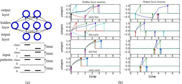
Figure 2: (a) Network implementing the XOR task using one hidden layer. There are 4 input patterns divided into two classes. (b) Post-training simulation results of the network in a for the four input patterns, one pattern per row. The left plots show the membrane potential of the four hidden layer neurons, while the right plots show the membrane potential of the two output layer neurons. Arrows at the bottom of the plot indicate input spikes to the layer, while arrows at the top indicate output spikes. The output spikes of the hidden layer are the input spikes of the output layer. The input pattern is indicated by the text in the left plots, and also by the pattern of input spikes.
4
Results
We trained the network to solve two classification tasks: an XOR task, and the permutation invariant MNIST task [11]. We used fully connected feedforward networks where the top layer had as many neurons as the number of classes (2 in the XOR task and 10 in the MNIST task). The goal is to train the network so that the neuron corresponding to the correct class fires first among the top layer neurons. We used the cross-entropy loss and interpreted the value of a top layer neuron as the negative of its spike time (in the z-domain). Thus, by maximizing the value of the correct class neuron value, training effectively pushes this neuron to fire earlier than the neurons representing the incorrect classes. For an output spike times vectorzLand a target class indexg, the loss function is given by
L(g,zL) =−ln exp(−z
L[g]) P
i
exp(−zL[i]) (10)
We used standard gradient descent to minimize the loss function across the training examples. Training was done using Theano [12, 13].
4.1 XOR task
In the XOR task, two spike sources send a spike each to the network. Each of the two input spikes can occur at time 0.0 (early spike) or 2.0 (late spike). The two input spike sources project to a hidden layer of 4 neurons and the hidden neurons project to two output neurons. The first output neuron must spike before the second output neuron if exactly one input spike is an early spike. The network is shown in Fig. 2a together with the 4 input patterns.
To investigate whether the network can robustly learn to solve the XOR task, we repeated the training procedure 1000 times starting from random initial weights each time. In each of these 1000 training trials, we used as many training iterations as needed for training to converge. Each training iteration involved presenting the four input patterns 100 times. Across the 1000 trials, the maximum number of training iterations needed to converge was61while the average was3.48. Figure 2b shows the
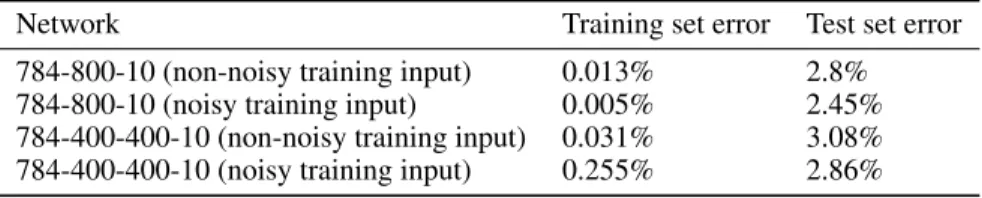
Table 1: Performance results for the permutation-invariant MNIST task
Network Training set error Test set error
784-800-10 (non-noisy training input) 0.013% 2.8% 784-800-10 (noisy training input) 0.005% 2.45% 784-400-400-10 (non-noisy training input) 0.031% 3.08% 784-400-400-10 (noisy training input) 0.255% 2.86%
post-training simulation results of the network when presented with each of the input patterns. The causal input sets of the different neurons change across the input patterns, allowing the network to implement the non-linearity needed to solve the XOR task.
4.2 MNIST classification task
The MNIST database contains 70,000 28x28 grayscale images of handwritten digits. The training set of 60,000 labeled digits was used for training, and testing was done using the remaining 10,000. No validation set was used. All grayscale images were first binarized to two intensity values: high and low. Pixels with high intensity generate a spike at time0, while pixels with low intensity generate a spike at timeln(6) = 1.79. All times are normalized with respect to the synaptic time constant (see Eq. 2). We investigated two feedforward network topologies with fully connected hidden layers: the first network has one hidden layer of 800 neurons (the 784-800-10 network), and the second has two hidden layers of 400 neurons each (the 784-400-400-10 network). We found that accuracy is slightly improved if we use an extra reference neuron that always spikes at time 0 and projects through trainable weights to all neurons in the network. We ran 100 epochs of training with an exponentially decaying learning rate and a mini-batch size of 10. Each of the two network topologies was trained twice, once with non-noisy input spike times and once with noise-corrupted input spike times. In the noisy input case, noise delays each spike with the absolute value of a random quantity drawn from a zero mean, unity variance Gaussian distribution. Noise was only used during training. Table 1 shows the performance results for the two networks after the noisy and non-noisy training regimes. The small errors on the training set indicate the networks have enough representational power to solve this task, as well as being effectively trainable. The networks overfit the training set as indicated by the significantly higher test set errors. Noisy training input helps in regularizing the networks as it reduces test set error but further regularization is still needed. We experimented with dropout [14] where we randomly removed neurons from the network during training. However, dropout does not seem to be a suitable technique in our networks as it reduces the number of spikes received by the neurons, which would often prevent them from spiking. Effective techniques are still needed to combat overfitting and allow better generalization in these networks.
Figures 3a and 3b show the distribution of spike times in the hidden layers and the distribution of the times of the earliest output layer spike in the two networks. The later are the times at which the networks made a decision for the 10,000 test examples. Both networks were first trained using noisy input. For both topologies, the network makes a decision after only a small fraction of the hidden layer neurons have spiked. For the 784-800-10 topology, an output neuron spikes (a class is selected) after only 3.0% of the hidden neurons have spiked (on average across the 10,000 test set images), while for the 784-400-400-10 topology, this number is 9.4%. The network is thus able to make very rapid decisions about the input class, after approximately 1-3 synaptic time constants from stimulus onset, based only on the spikes of a small subset of the hidden neurons. This is illustrated in Figs. 3c and 3d which show the membrane potentials of 10 hidden neurons and the 10 output neurons. The spikes of the 10 hidden neurons do not factor into the network decision in this case as they all spike after the earliest output spike, i.e, after the network has already selected a class.
5
Discussion
We presented a form of spiking neural networks that can be effectively trained using gradient descent techniques. By using a temporal spike code, many difficulties involved in training spiking networks such as the discontinuous spike generation mechanism and the discrete nature of spike counts are avoided. The network input-output relation is locally linear after a transformation of the time variable.
0 1 2 3 4 5 6 7 8 9 0.0 0.1 0.2 0.3 0.4 0.5 0.6 0.7 0.8 0.9 768-400-400-10 Norma lized frequency Spike time
Hidden layers' spikes First output layer spike
(a) 0 1 2 3 4 5 0.0 0.2 0.4 0.6 0.8 1.0 1.2 1.4 Norma lized frequency 768-800-10 Spike time
Hidden layers' spikes First output layer spike
(b) 0 1 2 3 4 5 6 time 1.0 0.5 0.0 0.5 1.0 vmem (c) 0 2 4 6 8 10 time 1.0 0.5 0.0 0.5 1.0 vmem (d)
Figure 3: (a,b) Histograms of spike times in the hidden layers and of the time of the first output layer spike across the 10,000 test set images for two network topologies. Both networks generate an output spike (i.e, select a class) before most of the hidden layer neurons have managed to spike. (c) Evolution of the membrane potentials of 10 neurons in the second hidden layer of the 768-400-400-10 network in response to a sample image. Top arrows indicate the spike (threshold crossing) times. (d) Evolution of the membrane potentials of the 10 output neurons in the same network and for the same input image as in c. The earliest output neuron spikes (network selects a class) at time 2.5, i.e, before any of the 10 hidden neurons shown in c have spiked.
As the input spike times change, the causal input sets of the neurons change, which in turn changes the form of the linear input-output relation (Fig. 1). This is analogous to the behavior of networks using rectified linear units (ReLUs) [10] where changes in the input change the set of ReLUs producing non-zero output, thus changing the linear transformation implemented by the network.
Recordings from higher visual areas in the brain indicate these areas encode information about abstract features of visual stimuli as early as125msafter stimulus onset [15]. Given the typical firing rate of cortical neurons and delays across synaptic stages, this indicates rapid visual processing is mostly a feedforward process where neurons get to spike at most once [16]. The presented networks follow a similar processing scheme and could thus be used as a trainable model to investigate the accuracy-response latency tradeoff in feedforward spiking networks. Output latency can be reduced by using a penalty term in the cost function that grows with the output spikes latency. Scaling this penalty term controls the tradeoff between minimizing latency and minimizing error during training. We considered the case where each neuron in the network is allowed to spike once. The training scheme can be extended to the case where each neuron spikes multiple times. The time of later spikes can be differentiably related to the times of all causal input spikes (see Eq. 7).
The presented networks enable very rapid classification of input patterns. As shown in Fig. 3, the network selects a class before the majority of hidden layer neurons have spiked. This is expected as the only way the network can implement non-linear transformations (in the z-domain) is by changing the causal set of input spikes for each neuron, i.e, by making a neuron spike before a subset of its input neurons have spiked. This unique form of non-linearity not only results in rapid processing, but it enables the efficient implementation of these networks on neuromorphic hardware since processing can stop as soon as an output spike is generated. In the 784-800-10 MNIST network for example, the network classifies an input after only 25 spikes from the hidden layers (on average). Thus, only a small fraction of hidden layer spikes need to be dispatched and processed.
References
[1] Yann LeCun, Yoshua Bengio, and Geoffrey Hinton. Deep learning.Nature, 521(7553):436–444, 2015.
[2] D.E. Rumelhart and J.L. McClelland. Parallel distributed processing: explorations in the microstructure of cognition. Volume 1. Foundations. MIT Press, Cambridge, MA, USA, 1986. [3] S.M. Bohte, J.N. Kok, and Han La-Poutre. Error-backpropagation in temporally encoded
networks of spiking neurons. Neurocomputing, 48(1):17–37, 2002.
[4] P. O’Connor, D. Neil, S.-C. Liu, T. Delbruck, and M. Pfeiffer. Real-time classification and sensor fusion with a spiking deep belief network.Frontiers in Neuroscience, 7(178), 2013. [5] Peter U Diehl, Daniel Neil, Jonathan Binas, Matthew Cook, Shih-Chii Liu, and Michael Pfeiffer.
Fast-classifying, high-accuracy spiking deep networks through weight and threshold balancing. InInternational Joint Conference on Neural Networks (IJCNN), 2015.
[6] Yongqiang Cao, Yang Chen, and Deepak Khosla. Spiking deep convolutional neural networks for energy-efficient object recognition.International Journal of Computer Vision, 113(1):54–66, 2015.
[7] Ning Qiao, Hesham Mostafa, Federico Corradi, Marc Osswald, Fabio Stefanini, Dora Sum-islawska, and Giacomo Indiveri. A re-configurable on-line learning spiking neuromorphic processor comprising 256 neurons and 128k synapses. Frontiers in Neuroscience, 9(141), 2015. [8] D. Neil and S.-C. Liu. Minitaur, an event-driven FPGA-based spiking network accelerator. Very
Large Scale Integration (VLSI) Systems, IEEE Transactions on, PP(99):1–1, October 2014. [9] Ben Varkey Benjamin, Peiran Gao, Emmett McQuinn, Swadesh Choudhary, Anand R
Chan-drasekaran, J Bussat, R Alvarez-Icaza, JV Arthur, PA Merolla, and K Boahen. Neurogrid: A mixed-analog-digital multichip system for large-scale neural simulations.Proceedings of the IEEE, 102(5):699–716, 2014.
[10] Vinod Nair and G.E. Hinton. Rectified linear units improve restricted boltzmann machines. InProceedings of the 27th International Conference on Machine Learning (ICML-10), pages 807–814, 2010.
[11] Y. Le Cun, L. Bottou, Y. Bengio, and P. Haffner. Gradient-based learning applied to document recognition. Proceedings of the IEEE, 86(11):2278–2324, Nov 1998.
[12] Fr´ed´eric Bastien, Pascal Lamblin, Razvan Pascanu, James Bergstra, Ian Goodfellow, Arnaud Bergeron, Nicolas Bouchard, David Warde-Farley, and Yoshua Bengio. Theano: new features and speed improvements. arXiv preprint arXiv:1211.5590, 2012.
[13] James Bergstra, Olivier Breuleux, Fr´ed´eric Bastien, Pascal Lamblin, Razvan Pascanu, Guillaume Desjardins, Joseph Turian, David Warde-Farley, and Yoshua Bengio. Theano: a cpu and gpu math expression compiler. InProceedings of the Python for scientific computing conference (SciPy), volume 4, page 3. Austin, TX, 2010.
[14] Nitish Srivastava, Geoffrey Hinton, Alex Krizhevsky, Ilya Sutskever, and Ruslan Salakhutdinov. Dropout: A simple way to prevent neural networks from overfitting. The Journal of Machine Learning Research, 15(1):1929–1958, 2014.
[15] C.P. Hung, Gabriel Kreiman, Tomaso Poggio, and J.J. DiCarlo. Fast readout of object identity from macaque inferior temporal cortex. Science, 310(5749):863–866, 2005.
[16] S. Thorpe, A. Delorme, R. Van Rullen, et al. Spike-based strategies for rapid processing.Neural networks, 14(6-7):715–725, 2001.