Technical Report No. 29
LARGE-SCALE HYDROLOGICAL EXTREMES IN
EUROPE: PAST AND FUTURE SIMULATIONS
WATCH is an Integrated Project Funded by the European Commission under the Sixth Framework Programme, Global Change and Ecosystems Thematic Priority Area (contract number: 036946).
The WATCH project started 01/02/2007 and will continue for 4 years.
Title: Large-scale hydrological extremes in Europe: past and future simulations
Authors: Jennifer Williamson, Simon Parry, George Goodsell, Christel Prudhomme, Jamie Hannaford
Organisations: Centre for Ecology & Hydrology, Wallingford, UK
Submission date: July 2011
Function: This report is an output from Work Block 4; Extremes: frequency, severity and scale; tasks M4.1-10b: comparison of extremes as simulated-/observed in river basin studies and variability as observed at the regional scale; 1: Future changes in droughts and M4.3-2: Future changes in large-scale flooding.
Deliverable WATCH deliverables D4.3.1a: Assessment of the future change in major droughts and their main physical aspects, including an
assessment of the uncertainty and D4.3.1b: Assessment of the future change in major large-scale floods and their main physical aspects, including an assessment of the uncertainty.
Abstract
Eight global hydrological models (GHM): Jules, Orchidee, HTessel, H08, MPI-HM, LPJml, WaterGap and GWAVA, were assessed concerning their ability to reproduce European large scale drought and high flow events when using meteorological inputs either observed (as represented by the WATCH Forcing Data WFD) or simulated by three Global Circulation Models (GCM), ECHAM5, IPSL and CNRM run under historical emission scenarios (control runs). In addition, the same GHMs were run with future projections from the same GCMs run under the A2 emissions scenario from 2001 to 2100 and the characteristics of large scale hydrological events compared to those of historical runs.
The analysis of RDI and RHFI on six contrasting regions across Europe does not suggest that any particular GHM, or family of GHMs, better reproduce the spatial coherence of flow anomalies than any other. When driven by different modelled, rather than observed, climate for the 20th century, the
sensitivity of different GHMs to the climate input becomes more apparent. The difference in the characteristics of future large-scale hydrological events as simulated by different GCM/GHM
combinations is further increased, due to both climate projection uncertainty and GHM sensitivity. When future projections are analysed, results suggest that in temperate regions of Europe the number of large scale drought events is projected to increase by the end of the 21st century by most GCM/GHM
combinations. For large scale high flow events, the signal is less clear but suggests little change in the number of events. However, in north-west Scandinavia fewer drought events and more high flow events are projected, probably due to increases in temperature causing less snowfall and more meltwater in the system. A change in the seasonality of events is also projected to occur in the High Alps with more high flows during spring, possibly again due to the influence of a warmer climate.
This multi-model analysis has clearly highlighted that the uncertainty due to hydrological modelling in climate change impact studies, often assumed to be negligible compared to that of climate modelling, can be large (and sometimes larger than that of GCMs) and should not be ignored.
1.
Introduction
It is becoming apparent that the hydrological cycle is intensifying e.g. (Huntington, 2006; Stott et al., 2010) as a result of climatic changes and it is likely that, as the climate continues to change through the 21st
century, the intensification of the hydrological cycle will continue. An important aspect of the
intensification of the hydrological cycle is an increase in the number of drought and flood events and changes in these extreme events may be more easily detected than changes in mean flows (Sheffield and Wood, 2008; Wilby et al., 2008). From an anthropogenic point of view changes in the extreme high and low flows are more important than changes in mean flows, as droughts and floods have had a significant impact across Europe in recent years. Examples include the 2003 drought in Europe, which caused 15,000 excess deaths (Finket al., 2004) and cost the agricultural and forestry sectors
approximately 13.1 billion Euros; the 2007 floods in the UK that caused 15 fatalities (Marsh and Hannaford, 2008) and the 2002 floods in Central Europe that cost over 14 billion Euros and were associated with over 100 fatalities (Ulbrich et al., 2003). These examples show that future increases in drought and flood events could have severe environmental and economic consequences.
The use of the Regional Deficiency Index (RDI) and Regional High Flow Index (RHFI) to indicate the extent of regional low and high flows has been developed on a Europe-wide scale by a number of authors including Hannaford et al., (2011), Parry et al., (2010) and Prudhomme et al., (in press). Although the historical RDI and RHFI have been shown to be representative indicators of regional hydrological extreme events they are not in themselves extreme events, but are based on the 10% most extreme observed low and high flows respectively (Prudhomme et al., in press).
This study aims to compare the ability of eight global hydrological models (GHM) to reproduce past large scale low and high flow events in six regions across Europe when driven by meteorological data derived from observations and from simulations of the 20th and 21st century climate by three sets of Global
Climate Models (GCMs). The comparison of the characteristics of the European hydrological extremes generated from observed and simulated 20th century climate helps to assess whether the considered
GCMs are able to reproduce meteorological patterns causing large scale low and high flow events. Twenty-first century projections provide an insight into possible changes in hydrological extremes predicted to occur over the next 90 years.
2.
Data and Methods
2.1. Observed data
The streamflow data set used to evaluate the GHM simulations is described in detail in Prudhomme et al. (in press) and Hannaford et al. (2011). It is based on the dataset assembled by Stahl et al. (2010) with additional data sourced from UK benchmark catchments, a set of undisturbed catchments that have previously been used in UK trend analysis studies (Hannaford and Marsh, 2008), and from Banque Hydro in France (Prudhomme and Sauquet, 2006). Briefly, this dataset comprises catchments that have had minimal anthropogenic disturbances, and gauging stations deemed to have good hydrometric
performance and records covering the period 1961-2005 (Prudhomme et al., in press). 2.2. Simulated data
This study used outputs from eight GHMs described in the WaterMIP model inter-comparison project, which compared the performance of eleven hydrological models simulating hydrological processes on a global scale (Haddeland et al., in press). Three different model types were considered: land surface models (Jules, HTessel and Orchidee), hydrological models (WaterGap, LPJml, and GWAVA) and models with intermediate characteristics (H08 and MPI-HM). For details of the GHMs see Haddeland et
All GHMs have the same 0.5o spatial resolution and were initially run for the period 1963-2001 using the
same meteorological input data, the Watch Forcing Data (WFD) (Weedon et al., 2010). All of the GHMs but GWAVA were also run for the period 1965-2000 using meteorological inputs from three global climate models (GCMs): ECHAM5, CNRM and IPSL. Temperature and rainfall inputs from these models were bias-corrected using the WFD (Piani et al., 2008). However, as this bias-correction does not correct for uncertainties in the climate signal related to the choice of GCM (Hagemann et al., in press), differences in the GCMs abilities’ to reproduce the causative meteorological mechanisms associated with hydrological extremes can still emerge. For more details of the three GCMs used in this study see Hagemann et al., (in press). Finally the seven GHMs were also run using future climate for the period 2001-2100 simulated by the three GCMs run with the A2 scenario only (IPCC, 2000).
2.3. Regional deficiency and high flow indices
The Regional Deficiency Index (RDI) was developed by Stahl (2001) as a way of characterising drought within homogeneous regions and was adapted for high flows (RHFI) by Parry et al., (2010). These regional indices represent the proportion of a region experiencing ‘drought’ or ‘flood’ on each day. The methodology used in this study follows that described by Lloyd-Hugheset al., (2010) and Hannaford et al., (2011) on the European catalogue of regional droughts in Europe and adapted by Prudhomme et al., (in press) for high flows.
The construction of the RDI and RHFI time series follows three steps, given in detail by Prudhommeet al., (in press) and explained briefly below (the alternative methodology for RHFI is given in parentheses). The first step for the observed data is the definition of a daily binary deficiency (exceedance) index DI (EI) time series. For each river flow record the daily flow is compared to a daily varying Q90 (Q10) threshold, which corresponds to the flow exceeded 90% (10%) of the time. In this study the flow that is exceeded 90% of the time, Q90, is the threshold for the DI and the flow that is exceeded 10% of the time, Q10, is the threshold for the EI. These thresholds are defined as follows: for a given day of the year (d) the daily-varying Q90(d) (Q10(d)) is calculated by ranking the historical flows across the 31 days centred on day d. This 31 day window increases the sample size and robustness of the estimate of Q90 (Q10). The second step is the grouping of sites based on the DI (EI) using a cluster analysis (Prudhomme et al., in press; Prudhomme and Sauquet, 2006; Stahl, 2001). The clustering was performed by applying a hierarchical technique using the Ward method and a binary Euclidean distance measure. The regions produced were predominantly spatially continuous and very similar for high and low flows so the regions were defined based on the DI. Finally RDI (RHFI) time series were defined for each region as the arithmetic mean of the DI (EI) series of all sites within the region for each day of record. The RDI(d) (RHFI(d)) represents the proportion of catchments in a region that experience flows that are below (above) the threshold on a given day (d) and expresses the spatial coherence of a large scale flow anomaly. The values for RDI and RHFI are between 0 and 1 with values of 0 meaning that none of the catchments in a region are experiencing low (high) flows and values of 1 meaning that all of the catchments in a region are experiencing low (high) flows (Prudhomme et al., in press).
For the data sets simulated by GHMs covering the control period (1963-2000) RDI (RHFI) time series were derived using a similar procedure to that described above but using the sum of the surface and subsurface runoff with thresholds calculated per grid cell rather than by catchment. The RDI (RHFI) time series were calculated for each region by considering all of the grid cells that have a centroid within the geographical boundary of the region (Prudhomme et al., in press). For the 21st century time series the
Prudhomme et al,. (in press). These regions are: south-east Great Britain, north-west Spain, western and central France, the High Alps, eastern Germany and the Czech Republic, and north-west Scandinavia. 2.4. Defining a discrete large scale drought (high flow) event
For the time series of the RDI (RHFI) the magnitude of the daily RDI (RHFI) expresses the spatial coherence of a drought (high flow) event, while the duration of the RDI (RHFI) values persisting above a given spatial coherence threshold shows the length of an event. Individual, spatially coherent drought (high flow) episodes can be identified by extracting independent and temporally coherent extreme values. The limit of spatial coherence used to define an event is based on the magnitude of the RDI (RHFI) and can either be fixed at a chosen value, which then allows comparison of the spatial coherence between regions, or can be selected based on a percentage of RDI (RHFI) values in each region to ensure that there are drought events selected in each region. In the following, we focus on large scale hydrological extremes as periods with the greatest spatial coherence based on days within the 10% and 5% largest RDI and RHFI, respectively. This selection method was chosen because the spatial coherence of drought events changes across Europe and it was considered more relevant to compare current and projected future events within each region than compare events between regions. Two large scale drought events are considered independent if separated by at least 85days. As large scale high flows are usually the result of much shorter meteorological extreme periods than droughts, a 10-day limit is chosen to distinguish two events.
3.
Large scale droughts
Large scale droughts simulated by GHMs were defined from RDI derived from the total simulated runoff as detailed above. Note that the minimum spatial coherence of events varies with each model run as it corresponds to the 10th percentile of the RDI. For 21st century simulations, the DI threshold is that of the
20th century simulations from the same GHM/GCM combination for comparison of projected changes in
extreme droughts.
3.1. Global Hydrological Models : evaluation using the WATCH Forcing Data
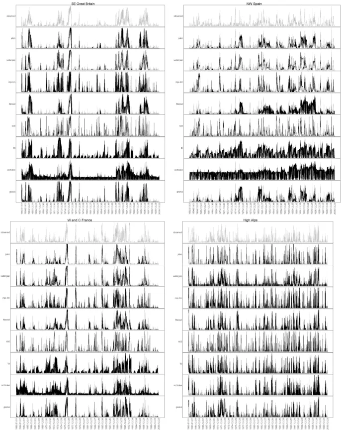
The GHMs were assessed by comparing Regional Deficiency Index (RDI) time series derived from observations (grey) and GHM simulations using WFD (black) shown together in Figure 1. As the WFD is derived from observations, the characteristics of the simulated drought events should be similar to those of observed RDI, both in terms of their regional coherence and their timing. For south-east Great Britain all GHMs approximately reproduce the observed drought periods with the exception of LPJml in 1990. For Orchidee and LPJml, however, RDI is never nil, suggesting there is always a portion of the region simulated to be under deficit; LPJml also shows a strong seasonal signal of dry summers. Conversely Jules and HTessel underestimate the short, less spatially coherent drought events. In north-west Spain none of the GHMs accurately reproduce the RDI time series derived from observations. Note, however, that due to the lack of available streamflow records in this region, it is possible that the RDI does not accurately represent all the true characteristics of droughts there. Any conclusion in this region should hence be treated with caution. In western and central France most of the major drought events are approximately reproduced by GHMs, although WaterGap, LPJml, GWAVA and, to a lesser extent Orchidee and Jules, all reproduce a drought event in the early 1970s that does not appear in the
observed record. Orchidee and LPJml overestimate the occurrence of less spatially coherent events and Jules and HTessel have a tendency to underestimate them. In eastern Germany and the Czech Republic WaterGap and H08 best reproduce the RDI time series, Jules and HTessel underestimate drought occurrence and the rest of the GHMs overestimate it. For the High Alps and north-west Scandinavia all of the GHMs except LPJml in Scandinavia approximately estimate drought occurrence, with LPJml showing
Figure 2 continued.
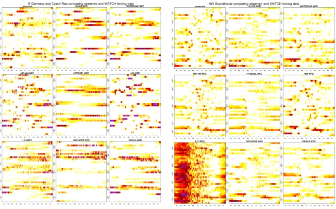
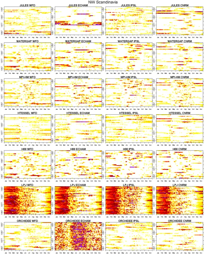
Figure 2 shows an alternative method of displaying the RDI time series, with the annual cycle on the x-axis and the year on the y-x-axis. For south-east Great Britain, western and central France, eastern Germany and the Czech Republic and the High Alps; WaterGap, HTessel and GWAVA reproduce the temporal patterns of drought anomalies seen in the observed record, while H08 and MPI-HM tend to produce short, highly-spatially coherent events compared to the observations. Jules over-estimates the length of the drought events in the High Alps and eastern Germany and the Czech Republic but does reproduce observed events well in western and central France and south-east Great Britain. LPJml and Orchidee overestimate the occurrence of drought events and underestimate their spatial coherence for all regions, with LPJml systematically simulating summers with more events than the observed dataset except in north-west Scandinavia, where long, spatially coherent winter droughts are simulated. This suggests that LPJml might not reproduce snowmelt and spring runoff processes accurately. In contrast to the other regions, drought patterns in north-west Scandinavia are best reproduced by H08.
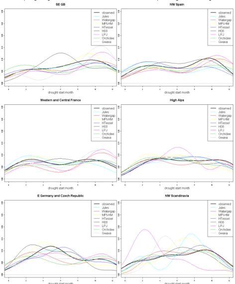
The seasonality of the onset of discrete drought events (see Section 2.4) is analysed using density plots of the month a drought event starts (Figure 3) and no single GHM is seen to consistently out-perform others. Jules best reproduces the seasonality in south-east Great Britain and eastern Germany, while MPI-HM performs best in north-west Spain, HTessel in western and central France, WaterGap in the High Alps and Orchidee in north-west Scandinavia. This suggests that different models simulate with different skill the hydrological processes at the start of a dry episode found in the contrasting regions. Although the timing of the drought events simulated by Orchidee is good in north-west Scandinavia, this model has showed some weaknesses in reproducing the magnitude and lengths of extreme drought events in other regions.
Figure 3: Date of the start of a drought event as identified from RDI time series derived from observations (black) and GHM simulations driven by the WATCH Forcing Data (colours) for six European regions. Regions and GHMs are as in Figure 1.
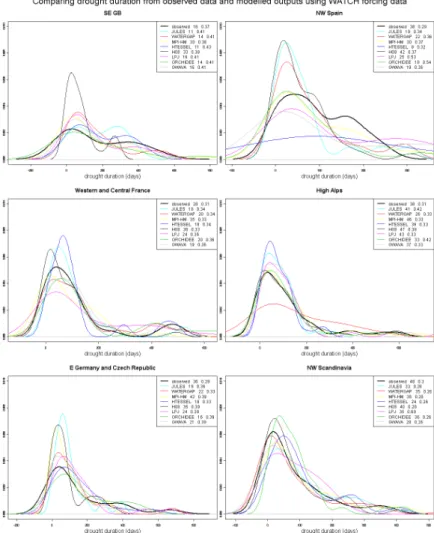
No single GHM consistently out-performs others when reproducing the length of discrete drought events (Figure 4). H08 systematically produces very short events across all of the regions, while Jules produces short events in Spain, western and central France and the High Alps but does reproduce the longer drought periods seen in south-east Great Britain. Except in the High Alps, Jules and HTessel produce too few separate events compared to the observed time series (see the legend in Figure 4 for the number of droughts simulated by each GHM). WaterGap and LPJml show a mixed performance across the six regions, with WaterGap performing particularly poorly in the High Alps. MPI-HM and Orchidee appear to reproduce the length of drought events best across the six regions, although Figure 2 shows that they do not reproduce the RDI time series derived from observations as well as some of the other models.
Figure 4: Duration (in days) of a drought event as identified from RDI time series derived from
observations (black) and GHM simulations driven by the WATCH Forcing Data (colours) for six European regions. Number of drought events between 1963 and 2000 and corresponding minimum spatial
coherence are given for all runs after GHM names. Regions and GHMs are as in Figure 1.
3.2. Global Hydrological Models: comparison using 20th century GCM simulations
The characteristics of drought events simulated by the GHMs driven by GCM climate are compared to those obtained from the same GHMs driven by the WFD. As the GHMs are unchanged, any differences in the RDI and associated drought events will result from differences in the driving climate. Although it is expected that the exact sequencing of drought events will vary (GCMs are designed to simulate the main statistical features of the climate and not the day-to-day weather), the number, intensity and seasonality of drought events should be similar across all input data types. Any differences due to the GHMs have been discussed in the previous section and are not dealt with in this section.
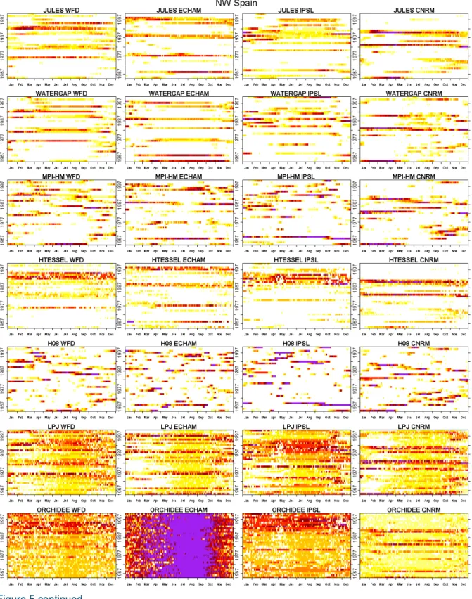
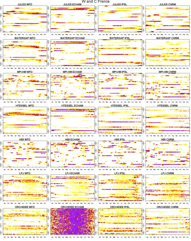
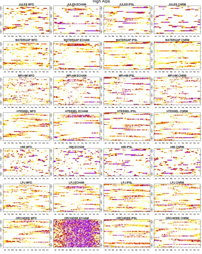
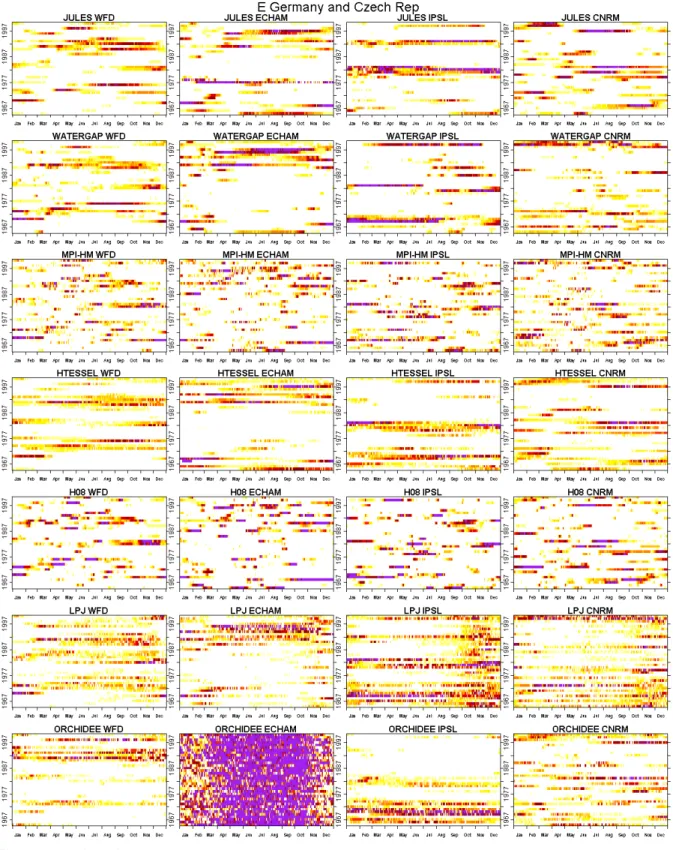
For Jules, WaterGap, MPI-HM, HTessel, H08 and LPJml, the RDI time series derived from the three GCMs’ 20th century driven runs are similar to those produced from the WFD time series across all six
regions (Figure 5). This suggests that there are no implicit biases in the climate of the control time period (20th century with historical emissions scenario) and that the climate as simulated by all three GCMs
(ECHAM5, CNRM and IPSL) has some meteorological characteristics compatible with the generation of extreme large scale drought events. However, the differences in the simulated climate can be highlighted
the record for that time of the year), IPSL climate resulting in RDI similar to those obtained with WFD and CNRM climate generating less spatially coherent RDI, suggesting higher runoff than that produced with the WFD.
Figure 5 continued.
Appendix 1 looks further at the 10% most spatially coherent drought events that occur in each region and compares the length and seasonality of those events. Across all regions and GCMs there are no
systematic biases, apart from results from Orchidee driven by ECHAM5 when a single event is simulated every year that lasts all though the summer.
3.3. Regional Deficiency Index: projections for the 21st century from GCM-driven GHMs
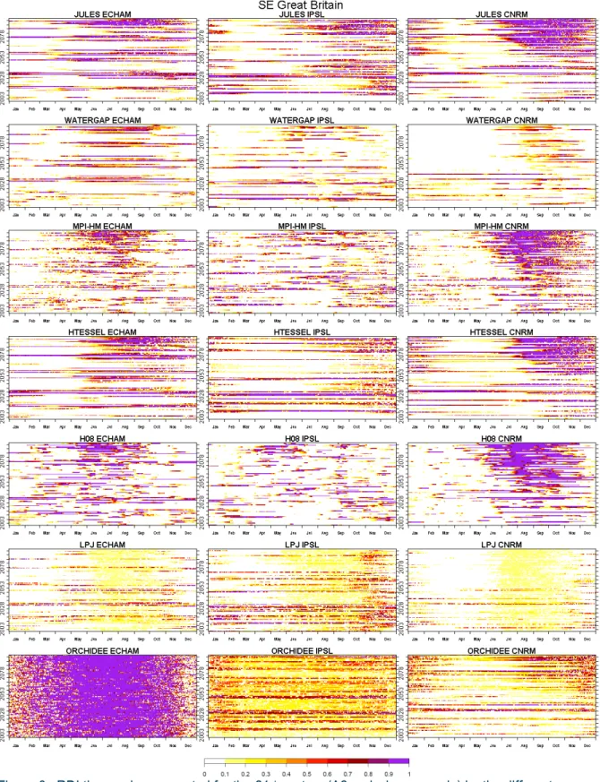
Figure 6 shows the Regional Deficiency Index time series obtained from GCM-driven GHMs total runoff for the period 2001-2100 (A2 emission scenario). For comparison with 20th century results, the deficit
periods were identified using the Q90 moving threshold defined from the 20th century simulations of the
same GCM/GHM combinations.
The magnitudes of RDI derived from ECHAM5/Orchidee 20th century simulation remain very high for the
21st century. Investigating further, the Q10 and Q90 thresholds used to define periods of runoff
deficit/exceedence are extremely small (and equal to zero for most regions for Q90) and very different from any other simulation. Those simulations should therefore be treated with caution.
In all regions except north-west Scandinavia, the CNRM-A2 future climate results in an increase in the frequency of drought events in summer and autumn from 2050 onwards when simulated by any GHM except LPJml. In north-west Scandinavia drought events are projected to occur earlier in the year, compared to other regions, possibly as a result of earlier onset of snow melt season due to warmer climate, resulting in future late spring flow lower than that of the 20th century. The CNRM-A2 future
climate also results in a marked reduction in winter and spring drought events over the same time period, possibly linked to warmer climate and subsequent higher winter and spring flow in the 21st compared to
the 20th century.
When driven by ECHAM5-A2 projections, all GHMs simulate a consistent annual drought period but centred on the summer months (June, July and August) rather than later in the year as projected by CNRM-A2. These events also become longer and more spatially coherent by the 2080s across all six regions and GHMs except for LPJml in north-west Scandinavia and Orchidee. It is not the aim of this report to investigate further the reasons leading to those differences, but because of the lack of consistency in the simulated RDI time series with LPJml and Orchidee when driven by different
meteorological data, conclusions in the changes projected by those GHMs must be treated with caution. Unlike CNRM-A2, ECHAM5-A2 does not result in a disappearance of winter droughts except in the High Alps and north-west Scandinavia, where the warmer climate is likely to be the cause of increased flow and decrease of the number of events of similar magnitude than those of the 20th century.
In contrast to the results obtained with CNRM-A2 and ECHAM5-A2, there is little seasonal pattern in future drought events simulated by any GHMs driven by IPSL-A2. In south-east Great Britain and the High Alps there is little sign of a change in frequency and spatial coherence of such events over the 21st
century. However, in the other four regions, drought events simulated by Jules, WaterGap, MPI-HM, HTessel and H08 tend to be longer and more spatially coherent towards the end of the 21st century.
Figure 6: RDI time series generated for the 21st century (A2 emission scenario) by the different
GHM/GCM combinations for the six study regions. Regions and GHMs are as in Figure 1. (Continued overleaf)
In north-west Spain and western and central France the number of drought events also increases although there is not such a marked change in seasonality between control and future periods. In
western and central France some GCM/GHM combinations show a progressive increase in the frequency of summer events, e.g. CNRM-A2 and ECHAM5-A2 with Jules, MPI-HM and HTessel; whereas in
contrast, IPSL-A2/LPJml simulates a shift towards autumnal episodes.
In contrast to the previous three regions, there are generally fewer projected drought events in the 2080s compared to the control time period in eastern Germany and the Czech Republic, but like south-east Great Britain there is a pronounced shift towards summer events in the 2080s.
In the High Alps the number of drought events does not change between the control period and the 2080s, but similarly to south-east Great Britain and eastern Germany and the Czech Republic, there is a
tendency for future events to cluster around a start date in late spring to mid summer.
Future drought events are projected to start in early summer in north-west Scandinavia. The number of drought events is not projected to change between the control and the 2080s and, for this region alone, the minimum spatial coherence of drought events (top 10th percentile of all RDI values) decreases for the
2080s (data not shown). A possible reason is the warmer climate resulting in more liquid water in the modelled system.
Figure 7: Seasonality of drought events’ start dates for the control (1965-1995, grey) and the future (2070-2100, red) time periods. The centre of the circle refers to 1965
4.
Large-scale high flows
Compared to regional drought time series it is more difficult to analyse regional high flows because they are generally of short duration, have a rapid onset and can often show spatial variability across a region, particularly when summer high flows are caused by convective storms.
4.1. Global Hydrological Models : evaluation using the WATCH Forcing Data
Figure 8 presents the Regional High Flow Index (RHFI) (x-axis with the annual cycle, y-axis the year of occurrence) for the six study regions as generated from the observed flow record and simulated by the eight Global Hydrological Models (GHM) driven by the WFD. For all regions except north-west
Scandinavia, MPI-HM, LPJml, Orchidee and GWAVA simulate high flow events that are too short and with very high spatial coherence compared to the observed data. In contrast, Jules and HTessel
generate high flows that are longer than the observed data but have a distinct period of very flashy, short duration high flows in late summer or early autumn, depending on the region. WaterGap tends to simulate high flow events that are too short in winter compared to the observed data but generates high flows that are more similar to the observed in the summer. H08 appears to simulate spatially coherent high flows in summer that are comparatively similar to those derived from the observed data and also produces a short period of spatially coherent high flows in winter, although to a greater extent than seen in the observed regions in most cases.
Figure 8 continued.
North-west Scandinavia shows slightly different results compared to the other five regions with Orchidee and GWAVA reproducing the observed RHFI time series fairly accurately, although with some short events in the summer. MPI-HM simulates high flow events that are too short compared to the observed time series, as does WaterGap during most high flow events. Jules, HTessel and H08 reproduce the
flow occurrence from then until 2001. These results suggest that in north-west Scandinavia only, all considered land surface models can reproduce the RHFI time series of the observed data more closely than the other types of GHM.
For Jules and HTessel, there is a peak in the number of discrete high flow events starting in late summer in south-east Great Britain, north-west Spain, western and central France and eastern Germany and the Czech Republic, while for WaterGap and MPI-HM, these episodes are prevalent in early spring in the same regions (Figure 9). When comparing the start date of the high flow events in north-west
Scandinavia GWAVA and Orchidee generate a summer peak in event frequency that is not seen in the observed data.
Figure 9: As figure 3 but for RHFI
Large scale high flow events derived from WFD-driven GHMs are systematically shorter and more numerous than when derived from observation data (Figure 10). HTessel best reproduces the number of events compared to the observed time series in all regions except north-west Spain, where WaterGap
Figure 10: As Figure 4 but for RHFI.
4.2. Global Hydrological Models: comparison using 20th century GCM simulations
All GHMs where driven by GCM meteorological data and the resulting RHFI was compared to those obtained with the same GHMs driven by WFD. Results show that WaterGap is the most sensitive to the climate model when looking at RHFI (Orchidee was the most sensitive model when analysing RDI). When driven by ECHAM5, RHFI are similar to those obtained with WFD, whereas when it is driven by IPSL or CNRM, WaterGap produces longer, spatially coherent high flows, with some short high flow episodes in winter (Figure 11). Orchidee also has a systematic bias when run with ECHAM5 with less simulated high flow events through the summer in all six regions. Note that Orchidee also produces almost continuous droughts through the summer when driven by ECHAM5.
In eastern Germany and the Czech Republic, the High Alps and north-west Scandinavia, Jules driven by IPSL generates a period of short high flows in January and February absent from results using WFD while when driven by ECHAM5 and CNRM, there are less, but longer, high flow events. This is also the case between July and October in south-east Great Britain, north-west Spain and western and central France.
Figure 11 continued.
Appendix 2 highlights the systematic bias in high flow simulations across the six regions by WaterGap. The seasonality of discrete high flow events generated by ECHAM5/WaterGap is similar to that obtained by WFD/WaterGap, whereas IPSL and CNRM inputs result in fewer events with a very different seasonal pattern between July and October in south-east Great Britain, north-west Spain and western and central France. No systematic biases in the seasonality of the high flows are apparent for other regions and
4.3. Future predictions for the 21st century
When generated using CNRM-A2 climate projections of the 21st century, and regardless of the GHM,
large scale high flow events become less frequent and severe during the summer and autumn, particularly from the 2050s onwards and more frequent and severe or of similar nature in the winter compared with the 20th century for all considered regions (Figure 12). A similar pattern occurs when all
GHMs except LPJml and Orchidee are driven by ECHAM5-A2 in all regions except eastern Germany and the Czech Republic. This is consistent with a “wetter winters, drier summers” scenario, often suggested to occur in Europe by 2100 (Christensen et al., 2007). However, this pattern is absent when GHMs are driven by IPSL-A2 highlighting the uncertainty in future climate projections.
The region with the greatest change in RHFI time series over time is north-western Scandinavia, with a large increase in winter high flow events in the second half of the 21st century suggested by all
GCM/GHM combinations. This is probably the result of an increase in temperature over the 21st century
causing earlier snowmelt and increased precipitation as rain rather than snow. These changes are simulated by all GHMs, suggesting that despite different formulations used in different GHMs to model the partitioning of water between solid and liquid (Haddeland et al., in press), runoff is systematically
simulated to increase in the future in high European latitudes. Note that projections from all three GCMs result in winter high flow events in this region becoming more spatially coherent and lasting longer from the 2050s onwards.
Figure 13 shows the seasonality of discrete high flow events over the control time period (grey) and the 2080s (red). Note that there are many more high flow events (as defined by periods with RHFI within the top 5th percentile) than drought events in the same time scale because of the shorter nature of high flows.
In south-east Great Britain there is a tendency for high flow events in the 2080s to be clustered in late winter and early spring, whereas events in the control time period are spread throughout the year with less seasonal clustering.
In north-west Spain and western and central France there appears to be little difference between the seasonality and number of high flow events between the control time period and the 2080s. Note however that the limit to define extreme high flow events is lower in the future for all GCM/GHM
combinations except for LPJml (data not shown), suggesting a decrease in the spatial coherence of large scale high flow events in the future in these regions.
In eastern Germany and the Czech Republic simulations driven by ECHAM5-A2 and CNRM-A2 results in a seasonal clustering of high flow events in winter and early spring. This is not seen with the IPSL-A2 projection, where, for most GHMs there is little seasonal structure to the data. The number of events remains relatively consistent between the control and the 2080s and the minimum spatial coherence defining a high flow event even increases with the IPSL-A2 driving climate for all GHMs, but decreases for all GHMS except WaterGap and LPJml when driven by ECHAM5-A2 or CNRM-A2.
CNRM-A2 inputs to the GHMs for the High Alps region result in a seasonal peak in high flow events in the winter and spring but this is not seen with ECHAM5-A2 or IPSL-A2 inputs except for WaterGap driven by IPSL-A2, which shows a strong seasonal shift towards winter high flow events. The number of high flow events remains relatively consistent between the two time periods but the minimum spatial coherence used to define each discrete event is projected to increase by almost all GCM/GHM combinations. This could be caused by higher temperatures and a subsequent increase in runoff due to snow and ice melt.
across this region is associated with a shift from shorter to longer events, although at the resolution of Figure 13 this cannot be seen.
5.
Conclusions
This study has assessed the ability of eight global hydrological models (GHM) to reproduce large scale hydrological extreme events across Europe, focussing on the spatio-temporal development of low and high flows, and investigated whether their characteristics might change in the future. The methodology is based on the concept of regionalised drought and high flow indices (RDI and RHFI) which measure the level of daily spatial coherence of runoff anomaly across a region, and from these indices extreme drought and high flow events are defined with the top 10th percentile and 5th percentile highest spatial
coherence, respectively. Analysis reported here focused on six contrasting regions.
Three land surface models were included within the GHM set: Orchidee, Jules and HTessel. Simulations generated by Orchidee are markedly different from those of other GHMs, particularly when driven by ECHAM5 meteorological data, where the Q10 and Q90 thresholds used to define periods of runoff deficit/exceedence are extremely small (and equal to zero for most regions for Q90). This is in contrast to the work done by Haddeland et al. (in press) who found that Orchidee simulates the highest global runoff fraction of all GHMs they considered when driven by the Watch Forcing Data. Until further investigation is made on the cause of these discrepancies, the simulations from Orchidee presented herein should be treated with caution.
The other two land surface models considered, Jules and HTessel, tend to produce longer, more spatially coherent events (both for drought and high flows) than any other GHM type. In contrast, the GHMs with a mix of characteristics (H08 and MPI-HM) tend to produce short, very spatially coherent events. Among the considered hydrological models, LPJml shows a strong seasonal drought signal with summer events occurring in most years across the regions when WFD and GCM inputs were used. Note this is not associated with any systematic absence of high flow events through the summer.
The analysis of RDI and RHFI on six contrasting regions across Europe does not suggest that any particular GHM, or family of GHMs, better reproduce the spatial coherence of flow anomaly than any other. When driven by different modelled, rather than observed, climate for the 20th century, the
sensitivity of different GHMs to the climate input becomes more apparent. The difference in the
characteristics of future hydrological events as simulated by different GCM/GHM combinations is further increased, due to both climate projection uncertainty and GHM sensitivity. A typical example is a strong pattern of ‘wetter winter, drier summers’ associated with more extreme high flow events in the winter and more drought events in the summer suggested when GHMs are driven by CNRM-A2. A similar pattern is apparent but less strong with ECHAM5-A2 data and absent from IPSL-A2-driven simulations. However, the difference between extreme events occurrence as simulated by the different GHMs remains very large.
When future projections are analysed, results suggest that in temperate regions of Europe the number of drought events is projected to increase by the end of the 21st century by most GCM/GHM combinations.
For high flow events, the signal is less clear but suggests little change in the number of events. However, in north-west Scandinavia fewer drought events and more high flow events are projected, probably due to increases in temperature causing less snowfall and more meltwater in the system. A change in the seasonality of large scale events is also projected to occur in the High Alps with more high flow events during spring, possibly again due to the influence of a warmer climate.
This multi-model analysis has clearly highlighted that the uncertainty due to hydrological modelling in climate change impact studies, often assumed to be negligible compared to that of climate modelling, can be large (and sometimes larger than that of GCMs) and should not be ignored. Future work should examine the role of the different hydrological model formulations in contributing to the large differences in low and high flow characteristics simulated by the GHMs analysed herein.
6.
References
Christensen JH, Hewitson B, Busuioc A, Chen A, Gao X, Held I, Jones R, Kolli RK, Twon W-T, Laprise R, Magaña Rueda V, Mearns L, Menéndez CG, Räisänen J, Rinke A, Sarr A, Whetton P (2007) Regional Climate Projections. in Solomon S, Qin D, Manning M, Chen Z, Marquis M, Averyt KB, Tignor M, Miller HL (eds.) Climate Change 2007: The Physical Science Basis. Contribution of Working Group I to the Fourth Assessment Report of the Intergovernmental Panel on Climate Change. Cambridge University Press, Cambridge, United Kingdom and New York, NY, USA, pp. 847-940.
Fink AH, Brucher T, Kruger A, Leckebusch GC, Pinto JG, Ulbrich U (2004) The 2003 European summer heatwaves and drought - synoptic diagnosis and impacts. Weather 59:209-216.
Haddeland I, Clark DB, Transsef W, Ludwig F, Voss F, Arnell NW, Bertrand N, Best M, Folwell S, Gerten D, Gomes S, Gosling SN, Hagemann S, Hanasaki N, Harding R, Heinke J, Kabat P, Koirala S, Oki T, Polcher J, Stacke T, Viterbo P, Weedon GP, Yeh P (in press) Multi-model estimate of global terrestrial water balance: setup and first results. Journal of
Hydrometeorology Water and global change special collection:xxx-xxx.
Hagemann S, Chen C-L, Haerter JO, Heinke J, Gerten D, Piani C (in press) Impact of a
statistical bias correction on the projected hydrological changes obtained from three GCMs and two hydrology models. Journal of Hydrometeorology.
Hannaford J, Lloyd-Hughes B, Keef C, Parry S, Prudhomme C (2011) Examining the large-scale spatial coherence of European drought using regional indicators of precipitation and streamflow deficit. Hydrological Processes 25:1146-1162.
Hannaford J, Marsh TJ (2008) High flow and flood trends in a network of undisturbed catchments in the UK. International Journal of Climatology 28:1325-1338.
Huntington TG (2006) Evidence for the intensification of the global water cycle: Review and synthesis. Journal of Hydrology 319:83-95.
IPCC (2000) Special report on emissions scenarios (SRES): A special report of Working Group III of the Intergovernmental Panel on Climate Change. Cambridge University Press, Cambridge. Lloyd-Hughes B, Prudhomme C, Hannaford J, Parry S, Keef C, Rees HG (2010) Drought catalogues for UK and Europe. Environment Agency Science Report SC070079/SR. Environment Agency, Bristol.
Marsh TJ, Hannaford J (2008) The 2007 summer flood in England and Wales - a hydrological appraisal. Centre for Ecology and Hydrology, p. 32.
Piani C, Haerter JO, Hagemann S, Allen M, Rosier S (2008) Practical methodologies to correct biases in climate model output, and to quantify and handle resulting uncertainties in estimates of future components of the global water cycle - WATCH Technical report 6. p. 17.
Prudhomme C, Parry S, Hannaford J, Clark DB, Hagemann S, Voss F (in press) How well do large-scale models reproduce regional hydrological extremes in Europe? Journal of
Hydrometeorology:xxx-xxx.
Prudhomme C, Sauquet E (2006) Modelling a regional drought Index in France. CEH/Cemagref report, p. 42.
Sheffield J, Wood EF (2008) Projected changes in drought occurrence under future global warming from multi-model, multi-scenario, IPCC AR4 simulations. Climate Dynamics 13:79-105.
Stahl K (2001) Hydrological drought - a study across Europe, Albert-Ludwigs Universität Freiburg, Freiburg.
Stahl K, Hisdal H, Hannaford J, Tallaksen LM, van Lanen HAJ, Sauquet E, Demuth S, Fendekova M, Jódar J (2010) Streamflow trends in Europe: evidence from a dataset of near-natural catchments. Hydrol. Earth Syst. Sci. 14:2367-2382.
Stott PA, Gillett NP, Hegerl G, Karoly DJ, Stone PH, Zhang XC, Zwiers FW (2010) Detection and attribution of climate change: a regional perspective. Wiley Interdisciplinary Reviews: Climate Change 1:192-211.
Ulbrich U, Brucher T, Fink AH, Leckesbuch GC, Kruger A, Pinter JG (2003) The central European floods of August 2002: Part 1, rainfall and flood development. Weather 58:371-377. Weedon GP, Gomes S, Viterbo P, Osterle H, Adam JC, Bellouin N, Boucher O, Best M (2010) The WATCH forcing data 1958-2001: a meteorological forcing dataset for land surface and hydrological models - WATCH Technical report 22. p. 41.
Wilby RL, Beven KJ, Reynard NS (2008) Climate change and fluvial flood risk in the UK: more of the same? Hydrological Processes 22:2511-2523.
Apr
Seasonality plots showing the onset and length of extreme drought events over the time period 1963-2000. The distance