Hybrid non-dominated sorting genetic algorithm with adaptive operators selection

Accepted Manuscript

Title: Hybrid Non-dominated Sorting Genetic Algorithm with

Adaptive Operators Selection

Author: W. Khan Mashwani Abdellah Salhi Ozgur Yeniay H.

Hussian M.A. Jan

PII:

S1568-4946(17)30106-0

DOI:

http://dx.doi.org/doi:10.1016/j.asoc.2017.01.056

Reference:

ASOC 4077

To appear in:

Applied Soft Computing

Received date:

14-9-2015

Revised date:

16-11-2016

Accepted date:

29-1-2017

Please cite this article as: W. Khan Mashwani, Abdellah Salhi, Ozgur Yeniay,

H. Hussian, M.A. Jan, Hybrid Non-dominated Sorting Genetic Algorithm with

Adaptive Operators Selection,

<![CDATA[Applied Soft Computing Journal]]>

(2017),

http://dx.doi.org/10.1016/j.asoc.2017.01.056

This is a PDF file of an unedited manuscript that has been accepted for publication.

As a service to our customers we are providing this early version of the manuscript.

The manuscript will undergo copyediting, typesetting, and review of the resulting proof

before it is published in its final form. Please note that during the production process

errors may be discovered which could affect the content, and all legal disclaimers that

apply to the journal pertain.

Accepted Manuscript

Highlights for HNSGA

ƒ

A novel hybrid non-dominated sorting genetic algorithm (HNSGA) for

multi-objective optimization with continuous variables is developed.

ƒ

HNSGA includes adaptive operator selection to allocate resources to multiple

search operators based on their individual performance at the subpopulation level.

ƒ

HNSGA is tested in classical benchmark problems taken from the ZDT and

&(&¶VXLWHV

ƒ

Inverted generational distance (IGD), relative hypervolume (RHV), Gamma and

Delta functions are used as performance indicators.

ƒ

The new algorithm is very competitive with other state-of-the-art optimizers such as

AMALGAM, NSGA-II, MOEA/D, Hybrid AMGA, OMOEA, PA-DDS etc.

Accepted Manuscript

Graphical Abstracts of the HNSGA Based on Adaptive

Operator Selection Strategy

The main goal of this paper is to investigate the effect of the multiple search operators with adaptive selection strategy and to develop hybrid version of non-dominated sorting genetic algorithm (HNSGA) for solving recently developed complicated multi-objective optimization test suit for multi-objective evolutionary algorithms (MOEAs) competition in the special VHVVLRQRIWKHFRQJUHVVRQHYROXWLRQDU\FRPSXWLQJKHOGDW1RUZD\LQ&(&¶7KH Inverted generational distance (IGD) has been used performance indicator to establish valuable comparison between the suggested algorithm and NSGA-II as shown in the figure below. A set of Pareto optimal solutions with smaller is the IGD values confirm that approximated Pareto front (PF) will cover whole part of true PF in term of proximity and diversity.

Accepted Manuscript

The average IGD-metric values evolution obtained by HNSGA versus NSGA-II for UF1-UF5 within allowable resources of 300,000 Function Evaluations.

Accepted Manuscript

Applied Soft Computing 00 (2017) 1–24

Applied

Soft

Computing

Hybrid Non-dominated Sorting Genetic Algorithm with Adaptive

Operators Selection

W.Khan Mashwani

a

, Abdellah Salhi

b

, Ozgur Yeniay

c

, H.Hussian

d

, M.A.Jan

e

a_{Department of Mathematics, Kohat University of Science&Technology, KPK, Pakistan}

E-mail:[email protected]

b_{Department of Mathematical Sciences, University of Essex, Colchester, UK,}

E-mail:[email protected]

c_{Department of Statistics, Hacettepe University, Beytepe Ankara Turkey,}

E-mail:[email protected]

d_{Technical Education&Vocational Training Authority, KPK, Pakistan}

E-mail:[email protected]

e_{Department of Mathematics, Kohat University of Science&Technology, KPK, Pakistan}

E-mail:[email protected]

Abstract

Multiobjective optimization entails minimizing or maximizing multiple objective functions subject to a set of constraints. Many real world applications can be formulated as multi-objective optimization problems (MOPs), which often involve multiple con-flicting objectives to be optimized simultaneously. Recently, a number of multi-objective evolutionary algorithms (MOEAs) were developed suggested for these MOPs as they do not require problem specific information. They find a set of non-dominated so-lutions in a single run. The evolutionary process on which they are based, typically relies on a single genetic operator. Here, we suggest an algorithm which uses a basket of search operators. This is because it is never easy to choose the most suitable operator for a given problem. The novel hybrid non-dominated sorting genetic algorithm (HNSGA) introduced here in this paper and tested on the ZDT (Zitzler-Deb-Thiele) and CEC’09 (2009 IEEE Conference on Evolutionary Computations) benchmark prob-lems specifically formulated for MOEAs. Numerical results prove that the proposed algorithm is competitive with state-of-the-art MOEAs.

c

2016 Elsevier Ltd. All rights reserved

Keywords: Multiobjective Optimization, Evolutionary Computation, Multiobjective Evolutionary Algorithms (MOEAs), Pareto Optimality, Adaptive Operator Selection.

1. Introduction

Multi-objective optimization deals with problems involving two or more conflicting objectives. In general, opti-mization problems can be combinatorial, continuous or both. The traveling salesman problem (TSP) [42] and mini-mum spanning tree (MST), for instance, are two well-known combinatorial problems. Combinatorial optimization has

various applications in air traffic routing, design telephonic networks, electrical, hydraulic, TV cables and computer

systems, road to deliver packages etc. Continuous optimization is widely utilized in mechanical design problems [24, 52]. This study is concerned with the minimization of multiple objectives within optimization problems (MOPs)

Accepted Manuscript

involving discrete and/or continuous variables. The general formulation of a MOP is vas follows.

minimize F(x)=(f1(x), . . . ,fm(x))T (1)

subject tox∈Ω

whereΩis the decision space, x= (x1,x2, . . . ,xn)T is a decision vector andxi,i =1, . . . ,nare decision variables,

F(x) :Ω →Rm_{includesmreal valued objective functions in the objective spaceR}m_{. IfΩis a closed and connected}

region inRn_{and all objective functions involve only continuous variables then problem (1) is a continuous MOP.}

In real-world multi-objective optimization problems, the objective functions are usually in conflict or mostly incommensurable. Consequently, there is not a unique solution that minimizes all the objective functions at the same time. The problem must be solved in terms of Pareto optimality.

A solutionu = (u1,u2, . . . ,un) ∈ Ω is said to be Pareto optimal if there does not exist another solutionv =

(v1,v2, . . . ,vn)∈Ωsuch that fj(u)≤ fj(v) for all j= 1, . . . ,mand fk(u) < fk(v) for at least indexk. An objective

vector is Pareto optimal if the corresponding decision vector is Pareto optimal. All Pareto optimal solutions in the decision space form a Pareto Set (PS) and their image in the objective space forms a Pareto Front (PF) [37, 9, 12].

In the last few year, several multi-objective evolutionary algorithms (MOEAs) were developed and successfully applied to various real-world optimization tasks [31, 36, 8, 6, 7, 27, 57, 30, 25]. Classical MOEAs can generally be categorized into three main paradigms such as Pareto dominance based MOEAs [13, 59, 58, 39, 17], indicator based evolutionary algorithms (IBEAs) [62, 63, 5, 3, 4, 14, 51] and decomposition based MOEAs [54, 23, 55, 32, 34, 29, 21].

Among decomposition methods, (MOEA/D) [54] is recently newly developed paradigm that transforms the given

MOP into a number of different single objective problems (SOPS) and then applies generic EA to simultaneously

optimize all these SOPs in single simulation runs to get optimal set solutions. MOEA/D has several enhanced variants

(e.g.[23, 55, 32, 34, 29, 21]). Decomposition and Pareto dominance approaches are the best choice for the adaptation of evolutionary operators and control parameters. IBEAs and decomposition based EAs do not use Pareto ranking directly as in Pareto dominance based MOEAs. All the above categorized MOEAs have two main goals: conver-gence towards the true Pareto front and maintaining a diverse set of solutions. They are population based stochastic techniques and approximate a set of optimal solutions in a single simulation run for the problem at hand. MOEAs

maintain diversity within this set of solutions using different measures such as the fitness sharing technique, the

nich-ing approach, the Kernel approach, the nearest neighbor approach, the histogram technique, the crowdnich-ing/clustering

estimation technique, the relaxed form of dominance and restricted mating and many others.

A fast non-dominated sorting genetic algorithm II (NSGA-II) [13], SPEA2 [58], Pareto archive evolution strat-egy (PAES) [22], multi-objective genetic algorithm (MOGA) [15], and niched Pareto genetic algorithm (NPGA) [17] are well known Pareto dominance based MOEAs. Among them, NSGA-II [13] is an improved version of the

non-dominated sorting genetic algorithm (NSGA)[20]. It generates offspring with crossover and mutation and

se-lects the next generation according to non-dominated sorting and crowding distance comparison. SPEA2 [58] is an improved version of strength Pareto evolutionary algorithm (SPEA) [60]. It incorporates a fine-grained fitness as-signment strategy, a density estimation technique, and an enhanced archive truncation method in contrast to SPEA [60]. Furthermore, it is equipped with the k-Nearest Neighbor (kNN) mechanism and a specialized ranking system to sort the members of the population, and select the next generation of population by combining the current population

and offspring population created via crossover and mutation. Both SPEA2 [58] and NSGA-II [13] showed excellent

performance in solving various real-world, scientific and engineering problems.

Memetic algorithms (MAs) are a growing area of research motivated by the meme notion introduced by Dawkins [38]. MAs are hybrid algorithms which combine local search optimizers and genetic algorithms. The first multi-objective MA was developed by Ishibuchi and Murata [18] and then improved by Jaszkiewicz [1, 19]. These

algo-rithms basically reformulate the given MOP into the simultaneous optimization of all weighted Tchebychefffunctions

or all weighted sum functions. The genetically adaptive multi-objective optimization algorithm (AMALGAM) [49]

blends multiple search operators to evolve new populations of solutions. The probability of the used different operators

are updated based on their particular current performances.

1.1. Motivation and Contributions

This paper presents a novel hybrid non-dominated sorting genetic algorithm (HNSGA) with an adaptive operator selection, inspired by evolutionary computing (EC) [49, 50, 29, 28, 32, 34, 35, 33]. The algorithm, developed starting

Accepted Manuscript

from NGSA-II [13], and uses multiple search operators such as simulated binary crossover (SBX) [11], differential

evolution (DE) [40], center of mass crossover (CMX) [46] and simplex crossover (SPX) [47] to evolve population evolution with a self-adaptive procedure.In particular, HNSGA divides candidate designs in subpopulations according

to number of operators, allocates different resources to each subpopulation in terms of selecting different search

operators for each subpopulation and updates size of each subpopulation. Using multiple search operators allows to increase the probability of selecting the most suitable operator for the problem at hand in each generation. Picking one operator at random or just because a search paradigm has always used is not really enough. The multioperator approach reduces the probability of selecting the wrong operator in the first place and increase our chances of using a more suitable operator for our problem, possibly the most suitable. The rate of use of an operator (i.e. the resources allocated in the optimization process for that operator) must depend on its performance. The best operators should work more in the optimization process. Should an operator work well in a generation it would be used in the next generation as well. This mechanism will be clarified in the pseudo-code of the proposed algorithm.

The main contributions of this paper are as follows.

• The suggested Hybrid NSGA employ multiple search operators based on adaptive procedure and its algorithmic

behavior is tested on classical benchmark problems such as the ZDT [61]and CEC09 problems [56].

• Optimization results are compared with those of state-of-the-art MOEAs such as NSGA-II [13], AMALGAM

[50], MOEA/D [55], hybrid archive-based micro genetic algorithm (AMGA) [45], orthogonal multi-objective

evolutionary algorithm (OMOEA) with lower-dimensional crossover [16], Pareto archived dynamically

dimen-sioned search (PA-DDS) with hypervolume based selection for multi-objective optimization [2], and diff

er-ential evolution with self-adaptation and local search for constrained multiobjective optimization algorithm (DECMOSA-SQP) [53].

• The inverted generational distance (IGD) [56], relative hypervolme (RHV) [48, 49], gammaΥ[13] and deltaΔ

[13] are used as performance indicators. In particular, IGD metric gives information on both convergence and spread of optimized solutions.

• It is found that HNSGA outperforms the above mentioned competitors as it always finds approximate Pareto

fronts (PF) closer to the true PF for most test problems.

The rest of the article is organized as follows. Section 2 outlines the new algorithm. Section 3 describes test problems and performance metrics. Section 4 presents and discusses optimization results. Section 5 summarizes the main findings of this study and outlines directions of future research.

2. Hybrid Non-dominated Sorting Genetic Algorithm with Adaptive Operators Selection

The pseudo-code of the proposed algorithm (HNSGA) is outlined in the Algorithm 1. HNSGA is an improved

version of NSGA-II [13]. Similar to NSGA-II [13], the present algorithm randomly generates a population setPtof

sizeN, uniformly distributed over the search space of the problem at hand.Thetsubscript denotes the number of the

current generation.

HNSGA initially divides the population Pt into q sub-populationsPt(k) whereq is the number of operators

selected for the search process. For example, if population size is N = 100 and there are 4 operators, it holds

Pt = [P1,P2,P3,P4] = [25,25,25,25]. The initial assignment of sub-populations to operators is not based on

fit-ness evaluation. Theq=4 search operators selected in this study are differential evolution (DE), simplex crossover

(SPX), simulated binary crossover (SBX) and center of mass crossover (CMX), respectively, for sub-populations 1,

2, 3 and 4.Each operator perturbs the designs included in its corresponding subset. For each sub-populationPt(k),an

offspring populationQt(k) is thus generated.The above mentioned tasks are completed in steps 4 through 26 of

Algo-rithm 1.Offsprings are merged in the populationQtincludingNelements.After first generation (t=1), sizes of thePk

sub-population sets are updated based on individual performances of theqoperator. NHSGA combines parent and

offspring populations into the populationRt=Pt∪Qtof size 2N.

In step 31, a fast non-dominated sorting procedure of NSGA-II [13] is applied to populationRand bestNsolutions

Accepted Manuscript

based on its contribution to the new population as outlined in Algorithm 2. Credit assignment procedures adopted

in HNSGA assign rewards to operators based on their offspring solutions that can survive to the next generation.

HNSGA counts the solution members ofQtretained in the new population `Ptand allocates 1smore of CPU time to

the operator that generated a trial solution able to replace a parent solution.Conversely, if the trial solution generated by an operator did not improve current population, that operator does not get any reward and its allocated CPU time

is increased by 0s(i.e. it remains unchanged). The counting of solutions retained in the new population `Ptor each

operator is done in steps 33−34 of the Algorithm 2.For example,Pt=[30,23,21,26] indicates that 30 elements have

been extracted fromP1∪Q1, 23 elements fromP2∪Q2, 21 elements fromP3∪Q3and 26 elements fromP4∪Q4.

Therefore, the first crossover operator got a larger population than other search operators. Finally, HNSGA provides a set of non-dominated solutions as termination criteria are satisfied.

3. Test Problems and Performance Metrics

Since real-world problems usually include many objective functions, different test suites for MOPs have been

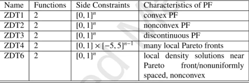
developed by evolutionary computation experts [10, 43]. In the present study, we have selected the ZDT [61] and CEC’09 [56] test problems. Their main features of ZDT problems are summarized in the Table 1 and CEC’09 test instances’s characteristics are explained in the Table 2.

Table 1. Characteristics of the Zitzler-Deb-Thiele’s (ZDT) Benchmark Functions

Name Functions Side Constraints Characteristics of PF

ZDT1 2 [0,1]n _{convex PF}

ZDT2 2 [0,1]n _{nonconvex PF}

ZDT3 2 [0,1]n _{discontinuous PF}

ZDT4 2 [0,1]×[−5,5]n−1 _{many local Pareto fronts}

ZDT6 2 [0,1]n _{local density solutions near}

Pareto front/nonuniformly

spaced, nonconvex

Table 2. Details of CEC’09 benchmark functions

CEC’09 Functions Side Constraints Characteristics of PF

UF1 2 [0,1]×[−1,1]n−1 _Concave

UF2 2 [0,1]×[−1,1]n−1 _Concave

UF3 2 [0,1]n _Concave

UF4 2 [0,1]×[−2,2]n−1 _Convex

UF5 2 [0,1]×[−1,1]n−1 _{21 point front}

UF6 2 [0,1]×[−1,1]n−1 _{One isolated point and two}

disconnected parts

UF7 2 [0,1]×[−1,1]n−1 _{Continuous straight line}

UF8 3 [0,1]2_×[−2,2]n−2 _Parabolic

UF9 3 [0,1]2_×[−2,2]n−2 _Planar

UF10 3 [0,1]2_×[−2,2]n−2 _Parabolic

MOEAs usually involve a number of internal parameters whose setting may greatly affect the computational

efficiency of the optimizer. In this study, experiment were carried out using the following values of the internal

parameters to solve the ZDT problems [61] and CEC’09 test instances [56].

• N=100: population size for 2-objective test instances.

• F=0.5: scaling factor of the DE;

Accepted Manuscript

Algorithm 1Hybrid Non-dominated Sorting Genetic Algorithm with Adaptive Operators Selection

1: [Input:]N: Population size,Pm: Probability of mutation,MaxGen: Maximum number of generations or

Termi-nation criterion,n: number of decision variables) andq=4 number of search operators.

2: [Output:] Pareto Set (PS)={x1_{, . . . ,x}N_{}and Pareto Front (PF)={F(x}1_{), . . . ,F(x}N_)};

3: Pt←Uniform-Random(N,n) Generate population setPtuniformly and randomly.

4: Evaluate-Fitness(Pt) Evaluate the fitness values ofPtsolutions.

5: Pt(k)← {N×1_q,k=1,2, . . . ,q} Select randomly equal number of solutions for each search operator att=1.

6: whileT ermination Condition is not S atis f ieddo

7: fori←1 :Ndo

8: ifi∈P1then

9: xj_,xk_,xi_{←Random-Selection(i,P1) such thatx}i_xj_xk_.

10: Q1←XOR1(xi,xj,xk) A CrossoverXOR1can be DE.

11: Q1_←Polynomial-Mutation(Q1_,Params) together withRepair-Strategy(Q1).

12: else

13: ifi∈P2then

14: xj_,xk_,xi_{←Random-Selection(i,P2) such thatx}i_xj_xk_.

15: Q2←XOR2(xi,xj,xk) XOR2can be SPX.

16: Q2←Polynomial-Mutation(Q2,Params) together withRepair-Strategy(Q2).

17: else

18: ifi∈P3then

19: xj_,xk_,xi_{←Random-Selection(i,P}

3) such thatxixjxk.

20: Q3←XOR3(xi,xj,xk) XOR3can be SBX.

21: Q3←Polynomial-Mutation(Q3,Params) together withRepair-Strategy(Q3).

22: else

23: ifi∈P4then

24: xj_,xk_,xi_{←Random-Selection(i,P4) such thatx}i_xj_xk_.

25: Q4←XOR4(xi,xj,xk) XOR4can be CMX.

26: Q4←Polynomial-Mutation(Q4,Params)←Repair-Strategy(Q4).

27: end if

28: end if

29: end if

30: end if

31: Qt←Combine-Offspring{Q1∪Q2∪Q3∪Q4} Combine sub-offspring population sets.

32: Evaluate-Fitness(Qt) Evaluate offspring populationQ.

33: end for

34: Rt←Combine-Parent-Offspring(Pt∪Qt) Combine parent and offspring populations.

35: Ranking+Crowding(Rt) Find ranks and measure crowding distance ofRtpopulation.

36: P`t←Select-Best-Individuals(Rt) SelectNbest Individuals fromRtpopulation.

37: {Ii|i = 1 : q} ← Count-Indices-XORs( `Pt) Count the individuals of each crossover to enter into new

populationP.

38: UpdatePt(k) For explanation go to Algorithm 2.

39: t=t+1;

Accepted Manuscript

Algorithm 2Adaptive Operators Selection Strategy

1: In steps 32 and 33 of Algorithm 1, we count the number of solutions of each operator that are retained in the new

population `Pin each generation of the algorithm.

2: Each successful solution generated by some operator leads to a reward of 1sfor that operator, while unsuccessful

solutions to a reward of 0sfor the operators that generated them. Here,sstands forseconds.

3: fork←1 :qdo

4: δ(k)←Count-Successful-Solutions( `P,q) Count the solutions of eachXORkcrossover that belong to `P.

5: ζ(k)←qδ(k) k=1δ(k)

;

6: Pt+1(k)←α×Pt(k)+(1−α)4ζk

k=1ζk ×N; whereαis a user defined parameter; hereα=0.2.

7: Update the resources allocation set of crossovers denoted byXOR

8: Pt(k)←Pt+1(k),k=1, . . . ,q

9: end for

• CR=0.5: probability of crossover;

• Feval=25000: maximum number of function evaluations;

• ηc = ηm =20 distribution indices for the SBX and polynomial mutation, whereηc measures the distance of

child solution from their parent solution andηmdefines the polynomial probability distribution.

• pc=0.7 andpm=1_n are probability of crossover and mutation, respectively.

Values of internal parameters for CEC’09 problems were instead set as follows.

• N=600: population size for 2-objective test problems;

• N=1000: for 3-objective test problems;

• F=0.5: scaling factor of the DE;

• CR=1: crossover probability for DE;

• Feval=300,000: maximum number of function evaluations;

3.1. Performance Metric

The quality of the final set of non-dominated solutions must be assessed in terms of convergence and diversity. The former depicts the closeness of the final set of non-dominated solutions to the true Pareto front (PF), while the latter aims to reach a uniform distribution of the final set of solutions over the true PF. Many performance metrics for measuring the quality of obtained solutions are suggested in the literature [41, 48, 12, 64]. Indicators including relative

hypervolume indicator (RHV) [48, 49], gamma (Υ) [13] and delta (Δ) [13] were used as indicators to quantitatively

assess performance of the used MOEAs in this paper.

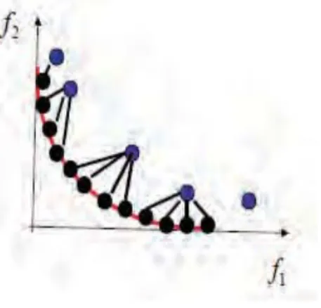
3.2. Inverted Generational Distance (IGD)

In this study, the inverted generational distance (IGD) [56] was utilized to evaluate the performance of the proposed algorithm. IGD measures both convergence and diversity of the approximate Pareto Front (APF) over the true PF.

Accepted Manuscript

Figure 1. Explanation of the inverted generational distance performance indicator.

LetP∗be a generated set of uniformly distributed points along the true PF (the black points) as shown in Figure

1. The average distance fromP∗to the approximated setA(the green points) is defined as [56]:

D(A,P)=

v∈P∗d(v,A) |P∗|

whered(v,A) is the minimum Euclidean distance betweenvand the points inA. IfP∗is large enough to represent the

PF very well,D(A,P) can measure both the diversity and convergence ofA: the smaller the value of the IGD metric

is, the better will be the obtained solution set. Here, we selectedP∗ =500 uniformly distributed solutions over the

true PF for two-objective problems andP∗=1000 individuals for problems with three objective functions.

3.3. Relative Hypervolume Indicator (RHV)

The relative hypervolume (RHV) indicator can mathematically be expressed as

RHV(A)= HV(P∗)−HV(A)

HV(P∗)

where (HV(.)) denotes the hypervolume of approximated setsAandP∗, calculated as follows [48, 49]:

HV(A)=volume∪|_iA₌|₁zi

wherei∈Aandziis theithhypercube constructed with respect to reference pointWand the solutionias the diagonal

corners of the hypercube.The approximated set of solutions will tend to the true Pareto-optimal set as the value of RHV tends to 0.

3.4. The Gamma (Υ) Indicator

In order to useΥmetric [13], P∗ = 500 uniformly spaced solutions were generated on the true Pareto-optimal

front of the problem at hand. For each solution included in the approximated setA, the minimum Euclidean distance

from the generated setP∗solution is computed. The average of these distances is defined as the is defined as gamma

Υmetric values. Hence, the approximated set will tend to the true Pareto-optimal set as theΥ-metric tends to 0.

Furthermore, this indicator measures the quality of convergence to a known set of Pareto-optimal solutions. The

smaller the value ofΥis, the better distribution and diversity of obtained non-dominated solutions will be. However,

since this metric sometimes cannot give information on the spread of obtained solutions, theΔ-metric was utilized in

Accepted Manuscript

3.5. The Delta (Δ) Indicator

TheΔmetric function is calculated as, [13]:

Δ =df+dI+

N−1

i=1 di−d

df+dI+(N−1)d ,

wheredfanddIare the Euclidean distances of the extreme solutions and the boundary solutions belonging to the

ap-proximated set of optimal solutions;ddenotes the average of all Euclidean distancesdibetween consecutive solutions

in the final approximated set of optimal solutions provided by a particular algorithm. Very small values ofΔresult in

better distribution and diversity of the approximated solution set.

4. Results and Discussion

The optimization algorithms compared in this study were coded in MATLAB and 30 independent optimization runs were performed for each test problem (with the parameter settings as specified in Section 3,consistently with the

values indicated in literature.) on a 2.4 GHz Core 2 Quad processor with 4 GB of RAM memory working on Windows

XP Professional Operating System.

Table 3 compares the minimum, median, mean, standard deviation and maximum IGD-metric values evaluated for the present HNSGA algorithm and other state-of-the-art MOEAs such as (a) HNSGA the suggested algorithm and

the state-of-the-art MOEAs: (b) AMALGAM [49], (c) NSGA-II [13], (d) MOEA/D [54] in the ZDT test problems

[10].It can be seen that HNSGA always found better approximated solutions set in terms of proximity to true PF and diversity. The same comparison is presented in the Table 4 with respect to the RHV-metric indicator while Table 5

evaluates the performance of HNSGA in terms ofΥandΔfunctions metrics. Again, the present algorithm was the

most efficient optimizer overall.

Table 6 statistically compare the IGD-metric values produced by HNSGA in the CEC’09 problems with those relative to several state-of-the-art algorithms such as ALMALGAM [49], NSGA-II-SQP [44], NSGA-II [13], hybrid AMAGA [45], OMOEA [16], PA-DS [2], and DECMOSA-SQP [53]. In order to have a homogeneous basis of comparison, HNSGA optimizations were run setting values of parameters shared with referenced algorithms equal to those indicated in the literature. It can be seen from the tables that HNSGA always was very competitive with other

optimizers outperforming other methods in most cases. Statistics expressed in terms ofΥandΔindicators (see Table

8) demonstrate that in the CEC’09 problems HNSGA could obtain a set of optimal solutions with better convergence properties spanning the solution sets over the entire Pareto-optimal region in most cases.

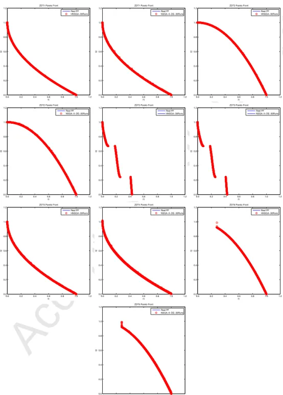
Figures 2 compares the best approximate Pareto fronts (PFs) of the five ZDT problems found by the HNSGA and NSGA-II [13] algorithms within 25000 function evaluations.It appears that the present algorithm can better reconstruct the true PF. The results obtained by HNSGA and NSGA-II [13] in the 30 independent simulations employing random seeds are compared in the Figures 3. It can be seen that all of the 30 PFs displayed for HNSGA entail a better distribution of solutions than in the case of NSGA-II [13].

Finally, Figure 4 compares the average variation of the IGD indicator for HNSGA and NSGA-II [13] confirming the superiority of the present algorithm that found the lowest values for this metric average variations in IGD-metric. The best approximate PFs found by HNSGA in the case of the CEC’09 test problems are shown in the Figures 5 while Figures 8 plots the corresponding results for NSGA-II [13]. In the present case, the best approximated PFs for the 2-objective function problems UF1-UF7 and the 3-objective function problems UF8-UF10) appear to be better in terms of diversity and proximity to true PF.

The PFs obtained in the 30 optimization runs of HNSGA are shown in the Figures 6 for problems UF1-UF4 and UF7- UF1-UF4, UF7-UF9. The corresponding plots for problems UF1-UF4 and UF7-UF10 solved with NSGA-II [13] are instead shown in Figure 7.

Figure 9 shows the evolution of the average IGD-metric with respect to the number of generations in problems UF1-UF7, UF9 and UF10. It can be seen that HNSGA always outperformed NSGA-II shows the average evolution in IGD-metric values versus number of generations spent by HNSGA and NSGA-II for dealing with UF1-UF7, UF9 and UF10. These figure demonstrate that HNSGA has tackled most test problems in much better average variation in the IGD-metric values as compared to NSGA-II.

Accepted Manuscript

Table 3. Statistical comparison of the IGD-metric values obtained by (a) HNSGA, (b) ALMALGAM [49], (c) NSGA-II [13] for ZDT problems.

CEC’09 Min Median Mean StD Max Algorithms

ZDT1 0.003764 0.003795 0.003804 0.000031 0.003912 a 0.004421 0.004623 0.004705 0.000237 0.005481 b 0.0042193 0.004472 0.004369 0.000139 0.004258 c 0.0040137 0.004196 0.004215 0.0001186 0.004557 d ZDT2 0.003852 0.003897 0.003897 0.000032 0.003975 a 0.004521 0.004893 0.004912 0.000269 0.005744 b 0.0043213 0.004649 0.004656 0.000182 0.005011 c 0.003837 0.003876 0.003886 0.0000426 0.004039 d ZDT3 0.0050394 0.0052055 0.0052010 0.00697 0.005359 a 0.004521 0.004893 0.004912 0.000269 0.005744 b 0.005132 0.00546 0.00912 0.01388 0.0602182 c 0.008484 0.009063 0.00915 0.000662 0.012523 d ZDT4 0.003811 0.003907 0.003921 0.000060 0.004145 a 0.004814 0.005297 0.005287 0.000171 0.005588 b 0.004814 0.005297 0.005287 0.000171 0.005588 c 0.011963 0.030562 0.042586 0.03342 0.157978 d ZDT6 0.003398 0.003448 0.003453 0.000032 0.003531 a 0.003821 0.004049 0.004055 0.000182 0.004732 b 0.005606 0.007045 0.007003 0.0005878 0.0080474 c 0.00856 0.015103 0.01479 0.004053 0.023509 d

Figure 10 visualize the contribution of each used crossover operator during the search process of the HNSGA to cope with tested MOPs. These figures demonstrate the adaptive searching behavior of the used crossover while

producing an successful offspring solutions to the next generation of population evolution in HNSGA framework.

The above discussed results confirm that HNSGA could reach global convergence and reconstruct the complete Pareto optimal frontier for almost all test problems selected from CEC’09 [56] and ZDT test suites [61]. However, the objective functions of problems UF5 and UF6 are multi-modal near the global Pareto-optimal frontier even and slight perturbations of optimization variables may cause solutions to become dominated and trapped in their local basin of attraction. Similar to its competitors, HNSGA faced genetic drift as population follows good solutions found in the early stages of search process. This results in the clustering of solutions around these early discovered points. The very good performance of HNSGA is mainly due to the use of multiple operators with self-adaptive strategies.

In fact, different operators may be suited for a larger variety of problems while the single operators utilized in the

other algorithms (e.g. NSGA-II [61]) may not keep best performance during the whole optimization process. For this reason, multiple ensemble search operators should be utilized for more complicated real-world problems than those considered in this study.

Accepted Manuscript

Table 4. Statistical comparison of the RHV-metric values obtained for (a) HNSGA, (b) ALMALGAM [49], (c) NSGA-II [13] for ZDT problems.

ZDT Min Median Mean StD Max Algorithms

ZDT1 0.0049897 0.0053957 0.0054043 0.0002026 0.0057415 a 0.0052387 0.0056880 0.0057441 0.0002893 0.0065897 b 0.0053851 0.0058431 0.0058705 0.0002625 0.0064456 c 0.0177029 0.020013 0.01991859 0.0004823 0.020497 d ZDT2 0.0049736 0.0051240 0.0051327 0.00002176 0.0052514 a 0.0050627 0.0055745 0.0056204 0.0002371 0.0061003 b 0.0052781 0.0057286 0.0057248 0.0002348 0.0061626 c 0.00505715 0.0051363 0.00514 0.00004208 0.0052718 d ZDT3 0.0029581 0.0032372 0.00326405 0.0001879 0.0038705 a 0.0032145 0.00354485 0.00356853 0.00020146 0.0039716 b 0.0051326 0.0054674 0.0091267 0.0138825 0.0602182 c 0.00477953 0.0048314 0.004828423 0.0001887 0.00483530 d ZDT4 0.0068649 0.0074254 0.0074463 0.0003463 0.0076536 a 0.0070600 0.0077258 0.0077495 0.0003516 0.00840719 b 0.0069089 0.0092493 0.0079564 0.0048926 0.0091253 c 0.0189880 0.0201214 0.020272 0.00060908 0.0218068 d ZDT6 0.0040689 0.0041922 0.0050197 0.0004514 0.0015346 a 0.0059667 0.0065878 0.0341751 0.1509787 0.8335517 b 0.006189 0.0069388 0.0068906 0.0003541 0.0077600 c 0.0048518 0.0050767 0.0052309 0.000459 0.0052243 d

Table 5. Statistical comparison of the_Υand_Δ-values for the ZDT problems [61].

ZDT Min Median Mean StD Max Metrics

ZDT1 0.0315434 0.0372392 0.0279883 0.0025911 0.0102020 Υ 0.2162211 0.30332014 0.3042615 0.01534164 0.3421585 Δ ZDT2 0.0142695 0.0215163 0.0234601 0.0047628 0.0284613 Υ 0.2264769 0.32186711 0.3231461 0.0231412 0.3603254 Δ ZDT3 0.0432680 0.0553217 0.0568125 0.0045721 0.0600402 Υ 0.449444 0.5045672 0.5046453 0.0202261 0.5131220 Δ ZDT4 0.0250162 0.0300238 0.0355547 0.0109218 0.0703774 Υ 0.3258961 0.3054030 0.3054483 0.0308418 0.4302315 Δ ZDT6 0.01034511 0.01504932 0.0151906 0.0057525 0.0316515 Υ 0.21454965 0.25196317 0.2538762 0.01027606 0.323209 Δ 10

Accepted Manuscript

Table 6. Statistical comparison of IGD-metric values obtained for (a) HNSGA, (b) ALMALGAM [49], (c) NSGA-II-SQP [44] (d) NSGA-II [13] on CEC’09 test instances.

CEC’09 Min Median Mean StD Max Algorithms

UF1 0.013033 0.012027 0.011238 0.001417 0.020143 a 0.029425 0.059633 0.057992 0.008557 0.070121 b 0.009851 ∗ ∗ ∗∗ 0.01153 0.0073 0.04734 c 0.051996 0.106873 0.096076 0.024862 0.128739 d UF2 0.003852 0.003897 0.003897 0.000032 0.003975 a 0.011432 0.013029 0.013217 0.001367 0.016769 b 0.006025 ∗ ∗ ∗∗ 0.01237 0.009108 0.05455 c 0.016012 0.019849 0.020050 0.001407 0.023589 d UF3 0.010300 0.027521 0.028749 0.013865 0.066973 a 0.091044 0.135348 0.136503 0.022927 0.199235 b 0.03435 ∗ ∗ ∗∗ 0.10603 0.06864 0.26207 c 0.066353 0.098234 0.097065 0.017958 0.134235 d UF4 0.040277 0.040458 0.041211 0.002399 0.059598 a 0.040359 0.041061 0.041020 0.000332 0.041678 b 0.04823 ∗ ∗ ∗∗ 0.0584 0.005116 0.06975 c 0.052199 0.054388 0.054551 0.001274 0.056679 d UF5 0.259499 0.376031 0.379204 0.065761 0.509010 a 0.166357 0.171420 0.171810 0.002873 0.178301 b 0.29106 ∗ ∗ ∗∗ 0.5657 0.1827 1.0498 c 1.523087 1.671735 1.676288 0.099452 1.844279 d UF6 0.077093 0.129060 0.150799 0.064798 0.281519 a 0.068589 0.079046 0.078552 0.005998 0.089807 b 0.08202 ∗ ∗ ∗∗ 0.31032 0.19133 0.71745 c 0.705834 0.762023 0.762271 0.028052 0.831784 d UF7 0.007499 0.009677 0.009788 0.000970 0.012891 a 0.014943 0.017678 0.017795 0.001254 0.020975 b 0.007631 ∗ ∗ ∗∗ 0.02132 0.01946 0.08801 c 0.067270 0.114403 0.112305 0.012055 0.125719 d UF8 0.090605 0.107091 0.08619 0.007010 0.123689 a 0.103736 0.234141 0.230682 0.026012 0.261557 b 0.06762 ∗ ∗ ∗∗ 0.0863 0.01243 0.10911 c 0.095436 0.108548 0.120433 0.030475 0.195112 d UF9 0.073649 0.106394 0.1120152 0.087431 0.320933 a 0.056616 0.067999 0.114652 0.085662 0.325894 b 0.03873 ∗ ∗ ∗∗ 0.0719 0.04504 0.19140 c 0.088857 0.188603 0.160832 0.047975 0.218993 d UF10 0.253304 0.307856 0.316548 0.020210 0.350921 a 0.273304 0.327886 0.326948 0.020030 0.360955 b 0.5339 ∗ ∗ ∗∗ 0.84468 0.1626 1.1266 c 0.473865 0.744428 0.781509 0.134987 1.043141 d

Accepted Manuscript

Table 7. Statistical comparison of IGD-metric values obtained for e) hybrid AMAGA [45], (f) Orthogonal MOEA (OMOEA) [16], (g) PA-DS with hypervolume based selection for multi-objective optimization [2], (h) DE with self-adaptation and local search for constrained multi-objective optimization (DECMOSA-SQP) [53] over 30 independent simulations on CEC’09 test instances [56].

CEC’09 Min Max Mean StD Algorithms

UF1 0.021023 0.059289 0.035886 0.010252 e 0.078362 0.096748 0.085646 0.004070 f 0.02909 0.10645 0.06234 0.02281 g 0.055126 0.0880129 0.0770281 0.039379 h UF2 0.011635 0.024160 0.016236 0.003167 e 0.027570 0.034295 0.030572 0.001609 f 0.00951 0.01909 0.01365 0.00232 g 0.0173361 0.040226 0.0283427 0.0313182 h UF3 0.037659 0.089363 0.069980 0.013954 e 0.201978 0.353186 0.271415 0.037612 f 0.08109 0.22473 0.12963 0.03291 g 0.0305453 0.168162 0.0935006 0.197951 h UF4 0.037688 0.044606 0.040621 0.001750 e 0.044441 0.048181 0.046246 0.000966 f 0.02927 0.03656 0.03229 0.00208 g 0.0316247 0.035643 0.0339266 0.0053707 h UF5 0.070599 0.134627 0.094057 0.0120555 e 0.163349 0.178052 0.169201 0.003901 f 0.13327 0.19261 0.21767 0.01718 g 0.133012 0.237081 0.167139 0.0895087 h UF6 0.045115 0.230019 0.129425 0.056588 e 0.068193 0.079371 0.073381 0.002448 f 0.06198 0.41434 0.22171 0.09903 g 0.0579174 0.589904 0.126042 0.561753 h UF7 0.013147 0.247734 0.057076 0.065309 e 0.031179 0.038803 0.033548 0.001735 f 0.13345 0.19234 0.21723 0.01709 g 0.0198913 0.0427502 0.024163 0.0223494 h UF8 0.139957 0.206937 0.171251 0.017224 e 0.139163 0.201114 0.192005 0.012296 f 0.08513 0.20854 0.13043 0.03932 g 0.0989388 0.228895 0.215834 0.121475 h UF9 0.112624 0.265932 0.188610 0.042137 e 0.105055 0.341103 0.231795 0.064767 f 0.02734 0.15901 0.04722 0.03041 g 0.0772668 0.332909 0.14111 0.345356 h UF10 0.201427 0.547349 0.324186 0.0957181 e 0.439716 1.082671 0.627544 0.145954 f 0.17627 0.74506 0.35129 0.20502 g 0.238279 0.580852 0.369857 0.65322 h 12

Accepted Manuscript

0.0 0.2 0.4 0,6 0.8 1.0 1.2 0.0 0.2 0.4 0,6 0.8 1.0 1.2 f1 f2 ZDT1 Pareto Front Real PF HNSGA 0.0 0.2 0.4 0,6 0.8 1.0 1.2 0.0 0.2 0.4 0,6 0.8 1.0 1.2 f1 f2 ZDT1 Pareto Front Real PF NSGA−II 0.0 0.2 0.4 0,6 0.8 1.0 1.2 0.0 0.2 0.4 0,6 0.8 1.0 1.2 f1 f2 ZDT2 Pareto Front Real PF HNSGA 0.0 0.2 0.4 0,6 0.8 1.0 1.2 0.0 0.2 0.4 0,6 0.8 1.0 1.2 f1 f2 ZDT2 Pareto Front Real PF NSGA−II 0.0 0.2 0.4 0,6 0.8 1.0 1.2 0.0 0.2 0.4 0,6 0.8 1.0 1.2 f1 f2 ZDT3 Pareto Front Real PF HNSGA 0.0 0.2 0.4 0,6 0.8 1.0 1.2 0.0 0.2 0.4 0,6 0.8 1.0 1.2 f1 f2 ZDT3 Pareto Front Real PF NSGA−II 0.0 0.2 0.4 0,6 0.8 1.0 1.2 0.0 0.2 0.4 0,6 0.8 1.0 1.2 f1 f2 ZDT4 Pareto Front Real PF HNSGA 0.0 0.2 0.4 0,6 0.8 1.0 1.2 0.0 0.2 0.4 0,6 0.8 1.0 1.2 f1 f2 ZDT4 Pareto Front Real PF NSGA−II 0.0 0.2 0.4 0,6 0.8 1.0 1.2 0.0 0.2 0.4 0,6 0.8 1.0 1.2 f1 f2 ZDT6 Pareto Front Real PF HNSGA 0.0 0.2 0.4 0,6 0.8 1.0 1.2 0.0 0.2 0.4 0,6 0.8 1.0 1.2 f1 f2 ZDT6 Pareto Front Real PF NSGA−II

Accepted Manuscript

0.0 0.2 0.4 0,6 0.8 1.0 1.2 0.0 0.2 0.4 0,6 0.8 1.0 1.2 f1 f2 ZDT1 Pareto Front Real PF HNSGA−30Runs 0.0 0.2 0.4 0,6 0.8 1.0 1.2 0.0 0.2 0.4 0,6 0.8 1.0 1.2 f1 f2 ZDT1 Pareto Front Real PF NSGA−II−DE−30Runs 0.0 0.2 0.4 0,6 0.8 1.0 1.2 0.0 0.2 0.4 0,6 0.8 1.0 1.2 f1 f2 ZDT2 Pareto Front Real PF HNSGA−30Runs 0.0 0.2 0.4 0,6 0.8 1.0 1.2 0.0 0.2 0.4 0,6 0.8 1.0 1.2 f1 f2 ZDT2 Pareto Front Real PF NSGA−II−DE−30Runs 0.0 0.2 0.4 0,6 0.8 1.0 1.2 0.0 0.2 0.4 0,6 0.8 1.0 1.2 f1 f2 ZDT3 Pareto Front Real PF HNSGA−30Runs 0.0 0.2 0.4 0,6 0.8 1.0 1.2 0.0 0.2 0.4 0,6 0.8 1.0 1.2 f1 f2 ZDT3 Pareto Front Real PF NSGA−II−DE−30Runs 0.0 0.2 0.4 0,6 0.8 1.0 1.2 0.0 0.2 0.4 0,6 0.8 1.0 1.2 f1 f2 ZDT4 Pareto Front Real PF HNSGA−30Runs 0.0 0.2 0.4 0,6 0.8 1.0 1.2 0.0 0.2 0.4 0,6 0.8 1.0 1.2 f1 f2 ZDT4 Pareto Front Real PF NSGA−II−DE−30Runs 0.0 0.2 0.4 0,6 0.8 1.0 1.2 0.0 0.2 0.4 0,6 0.8 1.0 1.2 f1 f2 ZDT6 Pareto Front Real PF HNSGA−30Runs 0.0 0.2 0.4 0,6 0.8 1.0 1.2 0.0 0.2 0.4 0,6 0.8 1.0 1.2 f1 f2 ZDT6 Pareto Front Real PF NSGA−II−DE−30Runs

Figure 3. Comparison of approximate Pareto fronts obtained in all optimization runs of HNSGA and NSGA-II on the ZDT problems

Accepted Manuscript

Table 8. Statistical comparison of the relative hypervolume (RHV) and gamma (_γ)-metric values obtained for HNSGA on CEC’09 test problems.

CEC’09 Min Median Mean StD Max Metrics

UF1 0.0101260 0.0109410 0.0108149 0.0682020 0.1020036 RHV 0.0108324 0.0237234 0.0239023 0.0120345 0.0210436 Υ UF2 0.0002587 0.0101630 0.0109421 0.0162106 0.0979968 RHV 0.0021431 0.00320010 0.0032022 0.0004012 0.0030416 Υ UF3 0.0013838 0.0021507 0.0021767 0.0003508 0.0030351 RHV 0.0103143 0.0123561 0.0124501 0.0020317 0.0134113 Υ UF4 0.0013838 0.0021507 0.0021767 0.0003508 0.0030351 RHV 0.0100453 0.0210312 0.0213969 0.0001301 0.0310281 Υ UF5 0.0307513 0.1208518 0.1314200 0.0401313 0.2087415 RHV 0.0361094 0.0317413 0.0375054 0.0212730 0.0624107 Υ UF6 0.0020242 0.0011711 0.0110571 0.1013035 0.6670742 RHV 0.0010155 0.0120732 0.0123627 0.0020207 0.0303115 Υ UF7 0.0003605 0.0009032 0.00921109 0.0102462 0.068491 RHV 0.0011005 0.0012051 0.0013203 0.0003216 0.0100234 Υ UF8 0.0421403 0.0986121 0.0985931 0.0001995 0.0990095 RHV 0.0011005 0.0012051 0.0013203 0.0003216 0.0100234 Υ UF9 0.0373526 0.0921153 0.0930047 0.0007384 0.0856440 RHV 0.0501054 0.5232083 0.5386664 0.0140512 0.0545365 Υ UF10 0.0003605 0.0009032 0.00921109 0.0102462 0.068491 RHV 0.095102 0.0932820 0.0943213 0.0004272 0.0672061 Υ 0 50 100 150 200 250 10−3 10−2 10−1 100 101 ZDT1 Number of Generations

AVG Variation in IGD Value

NSGA−II HNSGA 0 50 100 150 200 250 10−3 10−2 10−1 100 101 ZDT2 Number of Generations

AVG Variation in IGD Value

NSGA−II HNSGA 0 50 100 150 200 250 10−3 10−2 10−1 100 101 ZDT3 Number of Generations

AVG Variation in IGD Value

NSGA−II HNSGA 0 50 100 150 200 250 10−3 10−2 10−1 100 101 102 ZDT4 Number of Generations

AVG Variation in IGD Value

NSGA−II HNSGA 0 50 100 150 200 250 10−3 10−2 10−1 100 ZDT6 Number of Generations

AVG Variation in IGD Value

NSGA−II HNSGA

Accepted Manuscript

0.0 0.2 0.4 0,6 0.8 1.0 1.2 0.0 0.2 0.4 0,6 0.8 1.0 1.2 f1 f2

UF1 Pareto Front Real PF HNSGA 0.0 0.2 0.4 0,6 0.8 1.0 1.2 0.0 0.2 0.4 0,6 0.8 1.0 1.2 f1 f2

UF2 Pareto Front Real PF HNSGA 0.0 0.2 0.4 0,6 0.8 1.0 1.2 0.0 0.2 0.4 0,6 0.8 1.0 1.2 f1 f2

UF3 Pareto Front Real PF HNSGA 0.0 0.2 0.4 0,6 0.8 1.0 1.2 0.0 0.2 0.4 0,6 0.8 1.0 1.2 f1 f2

UF4 Pareto Front Real PF HNSGA 0.0 0.2 0.4 0,6 0.8 1.0 1.2 0.0 0.2 0.4 0,6 0.8 1.0 1.2 f1 f2

UF5 Pareto Front Real PF HNSGA 0.0 0.2 0.4 0,6 0.8 1.0 1.2 0.0 0.2 0.4 0,6 0.8 1.0 1.2 f1 f2

UF6 Pareto Front Real PF HNSGA 0.0 0.2 0.4 0,6 0.8 1.0 1.2 0.0 0.2 0.4 0,6 0.8 1.0 1.2 f1 f2

UF7 Pareto Front Real PF HNSGA 0.00.20.40,6 0.81.01.2 0.0 0.2 0.4 0,6 0.8 1.0 1.2 0.0 0.2 0.4 0,6 0.8 1.0 1.2 f1 UF8 Pareto Front

f2 Real PF HNSGA 0.00.20.40,6 0.81.01.2 0.0 0.2 0.4 0,6 0.8 1.0 1.2 0.0 0.2 0.4 0,6 0.8 1.0 1.2 f1 UF9 Pareto Front

f2 Real PF HNSGA 0.00.20.40,6 0.81.01.2 0.0 0.2 0.4 0,6 0.8 1.0 1.2 0.0 0.2 0.4 0,6 0.8 1.0 1.2 f1 UF10 Pareto Front

f2

Real PF HNSGA

Figure 5. Comparison of approximate Pareto fronts obtained in the best optimization run of HNSGA for the CEC’09 test problems.

Accepted Manuscript

0.0 0.2 0.4 0,6 0.8 1.0 1.2 0.0 0.2 0.4 0,6 0.8 1.0 1.2 f1 f2

UF1 Pareto Front Real PF HNSGA−30Runs 0.0 0.2 0.4 0,6 0.8 1.0 1.2 0.0 0.2 0.4 0,6 0.8 1.0 1.2 f1 f2

UF2 Pareto Front Real PF HNSGA−30Runs 0.0 0.2 0.4 0,6 0.8 1.0 1.2 0.0 0.2 0.4 0,6 0.8 1.0 1.2 f1 f2

UF3 Pareto Front Real PF HNSGA−30Runs 0.0 0.2 0.4 0,6 0.8 1.0 1.2 0.0 0.2 0.4 0,6 0.8 1.0 1.2 f1 f2

UF4 Pareto Front Real PF HNSGA−30Runs 0.0 0.2 0.4 0,6 0.8 1.0 1.2 0.0 0.2 0.4 0,6 0.8 1.0 1.2 f1 f2

UF7 Pareto Front Real PF HNSGA−30Runs 0.00.2 0.40,6 0.81.0 1.2 0.0 0.2 0.4 0,6 0.8 1.0 1.2 0.0 0.2 0.4 0,6 0.8 1.0 1.2 f1 UF8 Pareto Front

f2 Real PF HNSGA−30Runs 0.00.2 0.40,6 0.81.0 1.2 0.0 0.2 0.4 0,6 0.8 1.0 1.2 0.0 0.2 0.4 0,6 0.8 1.0 1.2 f1 UF9 Pareto Front

f2

Real PF HNSGA−30Runs

Accepted Manuscript

0.0 0.2 0.4 0,6 0.8 1.0 1.2 0.0 0.2 0.4 0,6 0.8 1.0 1.2 f1 f2

UF1 Pareto Front Real PF NSGA−II−30Runs 0.0 0.2 0.4 0,6 0.8 1.0 1.2 0.0 0.2 0.4 0,6 0.8 1.0 1.2 f1 f2

UF2 Pareto Front Real PF NSGA−II−30Runs 0.0 0.2 0.4 0,6 0.8 1.0 1.2 0.0 0.2 0.4 0,6 0.8 1.0 1.2 f1 f2

UF3 Pareto Front Real PF NSGA−II−30Runs 0.0 0.2 0.4 0,6 0.8 1.0 1.2 0.0 0.2 0.4 0,6 0.8 1.0 1.2 f1 f2

UF4 Pareto Front Real PF NSGA−II−30Runs 0.0 0.2 0.4 0,6 0.8 1.0 1.2 0.0 0.2 0.4 0,6 0.8 1.0 1.2 f1 f2

UF7 Pareto Front Real PF NSGA−II−30Runs 0.00.2 0.40,6 0.81.0 1.2 0.0 0.2 0.4 0,6 0.8 1.0 1.2 0.0 0.2 0.4 0,6 0.8 1.0 1.2 f1 UF8 Pareto Front

f2 Real PF NSGA−II−30Runs 0.00.2 0.40,6 0.81.0 1.2 0.0 0.2 0.4 0,6 0.8 1.0 1.2 0.0 0.2 0.4 0,6 0.8 1.0 1.2 f1 UF9 Pareto Front

f2 Real PF NSGA−II−30Runs 0.00.2 0.40,6 0.81.0 1.2 0.0 0.2 0.4 0,6 0.8 1.0 1.2 0.0 0.2 0.4 0,6 0.8 1.0 1.2 f1 UF10 Pareto Front

f2

Real PF NSGA−II−30Runs

Figure 7. Comparison of approximate Pareto fronts obtained in all optimization runs of NSGA-II on the CEC’09 test problems.

Accepted Manuscript

0.0 0.2 0.4 0,6 0.8 1.0 1.2 0.0 0.2 0.4 0,6 0.8 1.0 1.2 f1 f2

UF1 Pareto Front Real PF NSGA−II 0.0 0.2 0.4 0,6 0.8 1.0 1.2 0.0 0.2 0.4 0,6 0.8 1.0 1.2 f1 f2

UF2 Pareto Front Real PF NSGA−II 0.0 0.2 0.4 0,6 0.8 1.0 1.2 0.0 0.2 0.4 0,6 0.8 1.0 1.2 f1 f2

UF3 Pareto Front Real PF NSGA−II 0.0 0.2 0.4 0,6 0.8 1.0 1.2 0.0 0.2 0.4 0,6 0.8 1.0 1.2 f1 f2

UF4 Pareto Front Real PF NSGA−II 0.0 0.2 0.4 0,6 0.8 1.0 1.2 0.0 0.2 0.4 0,6 0.8 1.0 1.2 f1 f2

UF5 Pareto Front Real PF NSGA−II 0.0 0.2 0.4 0,6 0.8 1.0 1.2 0.0 0.2 0.4 0,6 0.8 1.0 1.2 f1 f2

UF6 Pareto Front Real PF NSGA−II 0.0 0.2 0.4 0,6 0.8 1.0 1.2 0.0 0.2 0.4 0,6 0.8 1.0 1.2 f1 f2

UF7 Pareto Front Real PF NSGA−II 0.00.20.40,6 0.81.01.2 0.0 0.2 0.4 0,6 0.8 1.0 1.2 0.0 0.2 0.4 0,6 0.8 1.0 1.2 f1 UF8 Pareto Front

f2 Real PF NSGA−II 0.00.20.40,6 0.81.01.2 0.0 0.2 0.4 0,6 0.8 1.0 1.2 0.0 0.2 0.4 0,6 0.8 1.0 1.2 f1 UF9 Pareto Front

f2 Real PF NSGA−II 0.00.20.40,6 0.81.01.2 0.0 0.2 0.4 0,6 0.8 1.0 1.2 0.0 0.2 0.4 0,6 0.8 1.0 1.2 f1 UF10 Pareto Front

f2

Real PF NSGA−II

Accepted Manuscript

0 100 200 300 400 500 10−3 10−2 10−1 100 101 UF1 Number of Generations

AVG Variation in IGD Value

NSGA−II HNSGA 0 100 200 300 400 500 10−3 10−2 10−1 100 UF2 Number of Generations

AVG Variation in IGD Value

NSGA−II HNSGA 0 100 200 300 400 500 10−2 10−1 100 101 UF3 Number of Generations

AVG Variation in IGD Value

NSGA−II HNSGA 0 100 200 300 400 500 10−2 10−1 100 UF4 Number of Generations

AVG Variation in IGD Value

NSGA−II HNSGA 0 100 200 300 400 500 10−2 10−1 100 101 UF5 Number of Generations

AVG Variation in IGD Value

NSGA−II HNSGA 0 100 200 300 400 500 10−2 10−1 100 101 UF6 Number of Generations

AVG Variation in IGD Value

NSGA−II HNSGA 0 100 200 300 400 500 10−3 10−2 10−1 100 101 UF7 Number of Generations

AVG Variation in IGD Value

NSGA−II HNSGA 0 50 100 150 200 250 300 10−2 10−1 100 101 UF9 Number of Generations

AVG Variation in IGD Value

NSGA−II HNSGA 0 50 100 150 200 250 300 10−1 100 101 102 UF10 Number of Generations

AVG Variation in IGD Value

NSGA−II HNSGA

Figure 9. Comparison of IGD-metric average values for HNSGA and NSGA-II [13] on the CEC’09 test instances.

5. Conclusion and Future Work

Recently, a variety of multi-objective evolutionary algorithms (MOEAs) have been developed and tested on di-verse test suites of MOPs including complicated real-world problems. Among these, the multi-objective evolutionary

algorithm based on decomposition (MOEA/D) [23] is a paradigm that transforms the given MOP into a number of

different single objective optimization problems (SOPS) and then applies a generic EA to simultaneously solve these

SOPs in a single simulation run aiming at getting the optimal set of solutions. MOEA/D has several enhanced versions

to be found in [26, 32, 29, 30, 27].

Pareto dominance based MOEAs do not rely on any decomposition strategy in their evolutionary process and solve MOP directly. Decomposition and Pareto dominance approaches are well suitable for the adaptation of evolutionary

operators and tuning of control parameters. NSGA-II [13] is one of the most popular and efficient Pareto dominance

based technique for dealing with diverse test suites of optimization and search problems.

This paper described a novel hybrid multiobjective evolutionary algorithm derived by combining NSGA-II, a state-of-the art Pareto dominance-based technique, with adaptive multiple operators selection strategy. The new algorithm,

Accepted Manuscript

0 500 1000 1500 2000 2500 10−2 10−1 100 UF1

Maximum Number of Generations

Probablity of Success of Crossovers in HNSGA.

CMX DE SPX SBX 0 500 1000 1500 2000 2500 10−2 10−1 100 UF2

Maximum Number of Generations

Probablity of Success of Crossovers in HNSGA.

CMX DE SPX SBX 0 500 1000 1500 2000 2500 10−2 10−1 100 UF3

Maximum Number of Generations

Probablity of Success of Crossovers in HNSGA.

CMX DE SPX SBX 0 500 1000 1500 2000 2500 10−2 10−1 100 UF4

Maximum Number of Generations

Probablity of Success of Crossovers in HNSGA.

CMX DE SPX SBX 0 500 1000 1500 2000 2500 10−2 10−1 100 UF5

Maximum Number of Generations

Probablity of Success of Crossovers in HNSGA.

CMX DE SPX SBX 0 500 1000 1500 2000 2500 10−2 10−1 100 UF6

Maximum Number of Generations

Probablity of Success of Crossovers in HNSGA.

CMX DE SPX SBX 0 500 1000 1500 2000 2500 10−2 10−1 100 UF7

Maximum Number of Generations

Probablity of Success of Crossovers in HNSGA.

CMX DE SPX SBX 0 500 1000 1500 10−2 10−1 100 UF8

Maximum Number of Generations

Probablity of Success of Crossovers in HNSGA.

CMX DE SPX SBX 0 500 1000 1500 10−2 10−1 100 UF9

Maximum Number of Generations

Probablity of Success of Crossovers in HNSGA.

CMX DE SPX SBX 0 500 1000 1500 10−2 10−1 100 UF10

Maximum Number of Generations

Probablity of Success of Crossovers in HNSGA.

CMX DE SPX SBX

Accepted Manuscript

called HNSGA, was tested in two sets of benchmark problems (the commonly used ZDT problems [61] and the

more difficult CEC’09 problems [61]) including 2 or 3 objective functions. It was found that the proposed approach

outperforms other state-of-the-art evolutionary algorithms with respect to robustness and capability of reconstructing the true Pareto front. In the future, the suggested algorithm will be used for solving combinatorial optimization problems and more complicated real-world problems including multiple objectives and constraints. Furthermore, multiple ensemble local search operators will be employed together with search operators to examine their strength in memetic computation.

References

[1] A.Jaszkiewicz, “Genetic Local search for Multi-objective Combinatorial Optimization,”European Journalof Operational Research, vol. 137, no. 1, pp. 50–71, 2002.

[2] M. Asadzadeh and B. Tolson, “Pareto Archived Dynamically Dimensioned Search with Hypervolume-based Selection for Multi-objective Optimization,”Engineering Optimization, vol. 45, no. 12, pp. 1489–1509, 2013.

[3] J. Bader, “Hypervolume-Based Search for Multiobjective Optimization: Theory and Methods,” Ph.D. dissertation, ETH Zurich, Switzerland, 2010.

[4] J. Bader and E. Zitzler, “HypE: An Algorithm for Fast Hypervolume-Based Many-Objective Optimization,”Evolutionary Computation, vol. 19, no. 1, pp. 45–76, 2011.

[5] N. Beume, B. Naujoks, and M. Emmerich, “SMS-EMOA: Multiobjective Selection based on Dominated hypervolume,”European Journal of Operational Research, vol. 181, no. 3, pp. 1653–1669, 2007.

[6] C.A.C.Coello and G. Lamont,Applications of Multi-objective Evolutionary Algorithms, ser. Advances in Natural Computation. World Scientific, Singapore, 2004.

[7] Carlos and R. L. Becerra, “Evolutionary Multi-Objective Optimization in Materials Science and Engineering,”Materials and Manufacturing Processes, vol. 24, no. 2, pp. 119–129, 2009.

[8] C. A. C. Coello, “A Comprehensive Survey of Evolutionary-Based Multiobjective Optimization Techniques,”Knowledge and Information Systems, vol. 1, pp. 269–308, 1999.

[9] C. A. Coello Coello, G. B.Lamont, and D. A. Veldhuizen,Evolutionary Algorithms for Solving Multi-Objective Problems. Kluwer Academic Publishers, New York, USA, 2002.

[10] K. Deb, L. Thiele, M. Laumanns, and E. Zitzler, “Scalable Multiobjective Optimization Test Problems,” vol. 1, pp. 825–830, 2002. [11] K. Deb,Multi-Objective Optimization using Evolutionary Algorithms, 1st ed. John Wiley and Sons, Chichester, UK, 2001.

[12] ——,Multi-Objective Optimization Using Evolutionary Algorithms, 2nd ed., S. Ross and R. Weber, Eds. John Wiley and Sons Ltd, 2002. [13] K. Deb, A. Pratap, S. Agarwal, and T.Meyarivan, “A Fast and Elitist Multiobjective Genetic Algorithm:NSGA-II,”IEEE Transactions on

Evolutionary Computation, vol. 6, no. 2, pp. 182–197, 2002.

[14] D.H.Phan and J.Suzuki, “R2-IBEA: R2 indicator Based Evolutionary Algorithm for Multiobjective Optimization,” inProceedings of the2013

IEEE Congress on Evolutionary Computation (CEC’13), 2013, pp. 1836–1845.

[15] C. Fonseca and P. Fleming, “An Overview of Evolutionary Algorithm in Multi-Objective Optimization,”Evolutionary Computation, vol. 3, no. 1, pp. 1–16, 1995.

[16] S. Gao, S. Zeng, B. Xiao, L. Zhang, Y. Shi, X. Tian, Y. Yang, H. Long, X. Yang, D. Yu, and Z. Yan, “An Orthogonal Multi-objective Evolutionary Algorithm with Lower-dimensional Crossover,” inProceedings of the2009IEEE Congress on Evolutionary Computation (CEC’09), 2009, pp. 1959–1964.

[17] J. Horn, N. Nafpliotis, and D. E. Goldberg., “A Niched Pareto Genetic Algorithm for Multiobjective Optimization,” inProceedings of the1st

IEEE Conference on Evolutionary Computation, CEC’94, 1994.

[18] H. Ishibuchi and T. Murata, “Multi-Objective Genetic Local Search Algorithm and Its Application to Flowshop Scheduling,”IEEE Transac-tions on Systems, Man and Cybernetics, vol. 28, no. 3, pp. 392–403, 1998.

[19] A. Jaszkiewicz, “On the Computational E_fficiency of Multiple Objective Metaheuristics. The Knapsack Problem Case Study,”European Journal of Operational Research, vol. 158, no. 2, pp. 418–433, 2004.

[20] K.Deb, “Multiobjective Genetic Algorithms: Problems Difficulities and Construction of Test Problems,”Evolutionary Computation, vol. 7, no. 3, pp. 205–230, 1999.

[21] W. Khan and Q. Zhang, “ MOEA_/D-DRA with Two Crossover Operators,” inProceedings of the UK Workshop on Computational Intelligence (UKCI 2010), 8th–10th September 2010, pp. 1–6.

[22] J. Knowles and D. Corne, “The Pareto Archived Evolution Strategy: A new Baseline Algorithm for Pareto Multiobjective Optimization,” in

Proceedings of the1999IEEE Congress on Evolutionary Computation (CEC’99), Piscatay, NJ, 1999, pp. 98–105.

[23] H. Li and Q. Zhang, “Multiobjective Optimization Problems With Complicated Pareto Sets: MOEA/D and NSGA-II,”IEEE Transactions on Evolutionary Computation, vol. 13, no. 2, pp. 284–302, 2009.

[24] X. Liao, Q. Li, X. Yang, W. Zhang, and W. Li, “Multiobjective Optimization for Crash Safety Design of Vehicles using Stepwise Regression Model,”Structural and Multidisciplinary Optimization, vol. 35, no. 6, pp. 561–569, 2008.

[25] C. Lucken, B. Barin, and C. Brizuela, “A Survey on Multi-Objective Evolutionary Algorithms for Many-objective Problems,”Computational Optimization and Applications, vol. 58, no. 3, pp. 707–756, 2014.

[26] W. K. Mashwani, “A Multimethod Search Approach Based on Adaptive Generations Level,” inProceedings of the7th_{International}

Confer-ence on Natural Computation(ICNC’11), Shanghai, China, 26-28 July, 2011, pp. 23–27.

[27] ——, “Hybrid Multiobjective Evolutionary Algorithms: A Survey of the State-of-the-art,”International Journal of Computer Science Issues, vol. 8, no. 6, pp. 374–392, 2011.

Accepted Manuscript

[28] ——, “Integration of NSGA-II and MOEA/D in Multimethod Search Approach: Algorithms,” inProceedings of the13th_{Annual Conference}

on Genetic and Evolutionary Computation, 2011, pp. 75–76.

[29] ——, “MOEA/D with DE and PSO: MOEA/D-DE+PSO,” inProceedings of the Thirty-first SGAI International Conference on Innovative Techniques and Applications of Artificial Intelligence, Cambridge, UK, December, 2011, pp. 217–221.

[30] ——, “Comprehensive Survey of the Hybrid Evolutionary Algorithms,”International Journal of Applied Evolutionary Computation (IJAEC), vol. 4, no. 2, pp. 1–19, 2013.

[31] ——, “Enhanced versions of Di_fferential Evolution: state-of-the-art survey,”International Journal Computing Sciences and Mathematics, vol. 5, no. 2, pp. 107–126, 2014.

[32] W. K. Mashwani and A. Salhi, “A Decomposition-Based Hybrid Multiobjective Evolutionary Algorithm with Dynamic Resource Allocation,”

Applied Soft Computing, vol. 12, no. 9, pp. 2765–2780, 2012.

[33] W. K. Mashwani, A. Salhi, M. A. Jan, R.A.Khanum, and M. Sulaiman, “Impact Analysis of Crossovers in Multiobjective Evolutionary Algorithm,”Science International Journal, Lahore, Pakistan, vol. 27, no. 6, pp. 4943–4956, 2015.

[34] W. K. Mashwani and A. Salhi, “Multiobjective Memetic Algorithm Based on Decomposition,”Applied Soft Computing, vol. 21, pp. 221–243, 2014.

[35] W. Mashwani, A. Salhi, M. Jan, R. Khanum, and M. Suliaman, “Enhanced Version of Genetically Adaptive Multi-Algorithm for Multiobjec-tive Optimization,”International Journal of Advanced Computer Science and Application, vol. 12, no. 6, pp. 279–287, 2015.

[36] ——, “Evolutionary Algorithms Based on Decomposition and Indicator Functions: State-of-the-art Survey,”International Journal of Ad-vanced Computer Science and Application, vol. 7, no. 1, pp. 1–11, 2016.

[37] K. M. Miettinien,Nonlinear Multiobjective Optimization, ser. Kluwer’s International Series. Norwell, MA: Academic Publishers Kluwer, 1999.

[38] P. Moscato. (2002, Jan 23) Memetic Algorithms’ Home Page. Http://alife.ccp14.ac.uk/memetic/www.densis.fee.unicamp.br/moscato/ memetic-home.html @ONLINE.

[39] N.Srinivas and K.Deb, “A Multiobjective Optimization using Nondominated Sorting in Genetic Algorithms,”Journal of Evolutionary Com-putation, vol. 2, no. 3, pp. 221–248, 1994.

[40] R.Storn and K.V.Price, “Di_fferential Evolution - a Simple and E_fficient Heuristic for Global Optimization over Continuous Spaces,”J.Global Opt, vol. 11, no. 4, pp. 341–359, December 1997.

[41] J. R. Schott,Fault Tolerant Design Using Single and Multicriteria Genetic Algorithm Optimization. Massachusetts Institute of Technology, Department of Aeronautics and Astronautics, 1995.

[42] A. Schuster and W¨urzburg, “About Travelling Salesmen and Telephone Network-Combinatirial Optimization at High School,”ZDM interna-tional Reviwer on Mathematical Education, vol. 36, no. 2, pp. 77–81, 2004.

[43] S.Huband, P.Hingston, and L. L.While, “A Review of Multiobjective Test Problems and a Scalable Test Problem Toolkit,”IEEE Transactions on Evolutionary Computation, vol. 10, no. 5, pp. 477–506, 2006.

[44] K. Sindhya, A. Sinha, K. Deb, and K. Miettinen, “Local Search Based Evolutionary Multi-objective Optimization Algorithm for Constrained and Unconstrained Problems,” inProceedings of the2009IEEE Congress on Evolutionary Computation, 2009, pp. 2919–2926.

[45] S. Tiwari, G. Fadel, P. Koch, and K. Deb, “Performance assessment of the hybrid Archive-based Micro Genetic Algorithm (AMGA) on the CEC09 test problems,” inProceedings of the2009IEEE Congress on Evolutionary Computation (CEC’09), 2009, pp. 1935–1942. [46] S. Tsutsui, “Multi-Parent Recombination in Genetic Algorithms with Search Space Boundary Extension by Mirroring,” inPPSN V:

Proceed-ings of the 5th International Conference on Parallel Problem Solving from Nature. London, UK: Springer-Verlag, 1998, pp. 428–437. [47] S. Tsutsui, M. Yamamura, and T. Higuchi, “Multi-Parent Recombination with Simplex Crossover in Real coded Genetic Algorithms,” in

Proceedings of the GECCO’99, 1999, pp. 657–374.

[48] D. A. V. Veldhuizen, “Multiobjective Evolutionary Algorithms: Classifications, Analyses, and New Innovations,” Graduate School of Engi-neering of the Air Force Institute of Technology Air University, Tech. Rep., 1999.

[49] J. A. Vrugt and B. A. Robinson, “Improved Evolutionary Optimization from Genetically Adaptive Mutimethod Search,”Proceedings of the National Academy of Sciences of the United States of America: PNAS (USA), vol. 104, no. 3, pp. 708–701, 2007.

[50] J. A. Vrugt, B. A. Robinson, and J. M. Hyman, “Self-Adaptive Multimethod Search for Global Optimization in Real-Parameter Spaces,”

IEEE Transactions on Evolutionary Computation, vol. 13, no. 2, pp. 243–259, 2009.

[51] M. Wagner, K. Bringmann, T. Friedrich, and F. Neumann, “Efficient Optimization of Many Objectives by Approximation-Guided Evolution,”

European Journal of Operational Research, vol. 243, no. 2, pp. 465–479, 2015.

[52] X. Yang,Engineering Optimization: An Introduction with Metaheuristic Applications, ser. Wiley Online Library: Books. Wiley, 2010. [53] A. Zamuda, J. Brest, B. Boskovic, and V. Zumer, “Differential Evolution with Self-adaptation and Local Search for Constrained Multiobjective

Optimization,” inProceedings of the 2009 IEEE Congress on Evolutionary Computation, 18-21 May, Trondheim, Norway, 2009, pp. 195–202. [54] Q. Zhang and H. Li, “MOEA/D: A Multiobjective Evolutionary Algorithm Based on Decomposition ,”IEEE transaction on Evolutionary

Computation, vol. 11, no. 6, pp. 712–731, December 2007.

[55] Q. Zhang, W. Liu, and H. Li, “The Performance of a New Version of MOEA_/D on CEC’09 Unconstrained MOP Test Instances,”Proceedings of the2009IEEE Congress On Evolutionary Computation, Trondheim, Norway, pp. 203–208, May, 18–21 2009.

[56] Q. Zhang, A. Zhou, S. Zhaoy, P. N. Suganthany, W. Liu, and S. Tiwariz, “Multiobjective Optimization Test Instances for the CEC 2009 Special Session and Competition,” Technical Report CES-487, 2009.

[57] A. Zhou, B.-Y. Qu, H. Li, S.-Z. Zhao, P. N. Suganthan, and Q. Zhang., “Multiobjective evolutionary algorithms: A survey of the state-of-the-art,”Swarm and Evolutionary Computation, vol. 1, pp. 32–49, 2011.

[58] E. Zitzler, M. Laumanns, and L. Thiele, “SPEA2: Improving the Strength Pareto Evolutionary Algorithm,” Computer Engineering and Networks Laboratory (TIK), ETH Zurich, Zurich, Switzerland, TIK Report 103, 2001.

[59] E. Zitzler and L. Thiele, “An Evolutionary Approach for Multiobjective Optimization: The Strength Pareto Approach,” Computer Engineering and Networks Laboratory (TIK), ETH Zurich, TIK Report 43, May 1998.

[60] ——, “An Evolutionary Approach for Multiobjective Optimization: The Strength Pareto Approach,” Computer Engineering and Networks Laboratory (TIK), ETH Zurich, TIK Report 43, 1998.

Accepted Manuscript

[61] E. Zitzler, K. Deb, and L. Thiele, “Comparsion of Multiobjective Evolutionary Algorithms: Emperical Results,”Journal of Evolutionary Computation, vol. 8, no. 2, pp. 173–195, 2000.

[62] E. Zitzler and S. Knzli, “Indicator-based selection in multiobjective search,” inin Proc. 8th International Conference on Parallel Problem Solving from Nature (PPSN VIII. Springer, 2004, pp. 832–842.

[63] E. Zitzler and S. Kunzli, “Indicator-Based Selection in Multiobjective Search,” inParallel Problem Solving from Nature - PPSN VIII, ser. Lecture Notes in Computer Science, X. Yao, E. Burke, J. Lozano, J. Smith, J. Merelo-Guervs, J. Bullinaria, J. Rowe, P. Tino, A. Kabn, and H.-P. Schwefel, Eds. Springer Berlin Heidelberg, 2004, vol. 3242, pp. 832–842.

[64] E. Zitzler, L. Thiele, M. Laumanns, C. M. Fonseca, and V. G. da Fonseca, “Performance Assessment of Multiobjective Optimizers: An Analysis and Review,”IEEE Transactions on Evolutionary Computation, vol. 7, pp. 117–132, 2003.