www.atmos-chem-phys.net/12/12243/2012/ doi:10.5194/acp-12-12243-2012
© Author(s) 2012. CC Attribution 3.0 License.
Chemistry
and Physics
Evaluation of the shortwave cloud radiative effect over the ocean by
use of ship and satellite observations
T. Hanschmann1, H. Deneke1, R. Roebeling2, and A. Macke1
1Leibniz-Institute for Tropospheric Research (TROPOS), Permoserstraße 15, 04318 Leipzig, Germany 2European Organization for the Exploitation of Meteorological Satellites (EUMETSAT), Darmstadt, Germany Correspondence to: T. Hanschmann ([email protected])
Received: 28 February 2012 – Published in Atmos. Chem. Phys. Discuss.: 19 July 2012 Revised: 29 November 2012 – Accepted: 10 December 2012 – Published: 21 December 2012
Abstract. In this study the shortwave cloud radiative
ef-fect (SWCRE) over ocean calculated by the ECHAM 5 cli-mate model is evaluated for the cloud property input de-rived from ship based measurements and satellite based esti-mates and compared to ship based radiation measurements. The ship observations yield cloud fraction, liquid water path from a microwave radiometer, cloud bottom height as well as temperature and humidity profiles from radiosonde ascents. Level-2 products of the Satellite Application Facility on Cli-mate Monitoring (CM SAF) from the Spinning Enhanced Visible and InfraRed Imager (SEVIRI) have been used to characterize clouds. Within a closure study six different ex-periments have been defined to find the optimal set of mea-surements to calculate downward shortwave radiation (DSR) and the SWCRE from the model, and their results have been evaluated under seven different synoptic situations. Four of these experiments are defined to investigate the advantage of including the satellite-based cloud droplet effective radius as additional cloud property. The modeled SWCRE based on satellite retrieved cloud properties has a comparable accuracy to the modeled SWCRE based on ship data. For several cases, an improvement through introducing the satellite-based esti-mate of effective radius as additional information to the ship based data was found. Due to their different measuring char-acteristics, however, each dataset shows best results for dif-ferent atmospheric conditions.
1 Introduction
Clouds strongly influence the energy budget of the Earth’s atmosphere. Because of their high degree of temporal and
spatial variability, and the complexity of cloud processes, it remains challenging to model and predict the effect of clouds on the energy budget. The representation of clouds in global circulation models (GCMs) are identified as the largest source of uncertainty for predicting future climate change by the International Panel on Climate Change and others (IPCC, 2007; Ramanathan et al., 1989). Especially the cloud radiative effect (CRE), defined as the difference be-tween the net radiative fluxes of the cloudy and cloud-free at-mosphere, is often not represented satisfactorily. The reason for this is its dependence on a large number of cloud param-eters and their highly variable distribution. These paramparam-eters include the vertical profiles of ice and liquid water, effective radius (re), and cloud droplet number concentration (CDNC). To evaluate this source of uncertainty in GCMs, it is impor-tant to identify those situations in which the model can re-produce the CRE well and badly. For this purpose, ground-based measurements as well as satellite ground-based estimates can be used (Macke et al., 2010a). Ground-based measurements are also needed to verify the accuracy of satellite products, which are generally based on more indirect retrieval tech-niques. Over ocean, however, which covers nearly 2/3 of the Earth, ground-based measurements of cloud properties and radiative fluxes are sparse.
Starting with the Meridional Ocean Radiation Experi-ment MORE (5 ship cruises; Sinitsyn et al., 2006; Macke et al., 2007) and continued with the OCEANET project (11 ship cruises; Macke, 2009; Macke et al., 2010a; Kalisch and Macke, 2012), a comprehensive data set has been established. OCEANET provides ship based mea-surements of cloud properties and radiative fluxes with high temporal resolution, including a total sky imager
(TSI; Kalisch and Macke, 2008, 2012), from all cruises. Ad-ditional instruments operated during some of the cruises in-clude a microwave radiometer (RPG HATPRO; Rose et al., 2005), a sun photometer for the MARITIME AEROSOL NETWORK (MAN/AERONET; Smirnov et al., 2009), a Ra-man lidar (Althausen et al., 2009), as well as instrumentation for measuring turbulent fluxes. Due to the cruise tracks the majority of clouds observed during OCEANET are relatively thin liquid water clouds, which still pose significant chal-lenges both to current measurement techniques and our sci-entific understanding of cloud-climate interactions (Turner et al., 2007).
Ebell et al. (2011) used atmospheres obtained from ground-based measurements over land for the calculation of the CRE, by feeding these measurements into a radiative transfer model (RTM). They concentrated on the Convec-tive and Orographically-induced Precipitation Study (COPS; Wulfmeyer et al., 2011) measurement site where a wide range of instruments including the Atmospheric Radiation Measurement Mobile Facility (AMF) were deployed. For single layer water clouds using the Rapid Radiative Transfer Model for GCMs (RRTMG; Clough et al., 2005) a bias be-tween the measured and modelled DSR of−39.1 W m−2was found in that study. Guo and Coakley (2008) compared ship-based radiation measurements for cloud free scenes against corresponding satellite based Clouds and Earth’s Radiant En-ergy System (CERES) estimates and RTM simulations, and found agreements better than 2 % relative to the model sim-ulations and between 2 and 3 % relative to the satellite es-timates. They took their model atmospheres from National Center for Environmental Prediction (NCEP) fields and a marine aerosol optical depth (AOD) of 0.05 at a wavelength of 0.55 µm was assumed.
Until now, the assessment of model-based cloud proper-ties over the ocean (e.g. as estimated by ISCCP; Rossow and Schiffer (1991)) and their associated cloud radiative effect (e.g. as observed by ERBE (Barkstrom , 1984) & CERES (Wielicki et al., 1996)) has mostly been based on satellite data sets, or on data of voluntary observing ships (e.g. Be-dacht et al., 2007). The observations collected on board of the Research Vessel (R/V) POLARSTERN facilitate such evalua-tions, and represent a unique dataset in terms of instrumental capabilities as well as temporal and spatial resolution.
The aim of this study is to test which dataset of observed cloud properties serves as best input to calculate the cloud radiative effect by the ECHAM-5 RTM, ship or satellite ob-servations. To this end different experiments with different combinations of measurements from ship and from satellite have been performed. This paper is structured as follows: an overview of the ship- and satellite-based data sets is pre-sented in the next section, followed by a description of the radiative transfer model used for our study. In the method-ology section the averaging technique and assumptions used in the RTM are described. In a closure study presented in Sect. 5, different experiments are carried out for
determin-ing the optimal input parameters to the RTM by compardetermin-ing modeled radiative fluxes to the ship measurements. Finally, discussions and conclusions are given in Sect. 6.
2 Data
Two different data sources are considered for this study. Ship data are used which resolve cloud radiative effects on small spatial and temporal scales. The ship-based atmo-spheric measurements are used as input for the RTM. The ship-based radiation flux measurements are used for valida-tion. The satellite retrievals of effective radius and liquid wa-ter path are used as alwa-ternative or additional RTM input. In the following both datasets (surface measurements and satel-lite products) and the algorithms used to derive them are de-scribed.
2.1 Ship measurements
Liquid water path (LWP), temperature, and humidity (T+H) profiles have been derived from a HATPRO microwave ra-diometer (Rose et al., 2005). A statistical retrieval is applied to the microwave radiometer (MWR) measurements, which relies on a training dataset to compute LWP and T +H -profiles from observed radiances. Errors in brightness tem-perature of 1 K lead to a maximum error of 30 g m2in LWP (Crewell and Loehnert, 2003). A pyranometer of type CM21 (Kipp and Zonen, 2004) is used to measure global radia-tive fluxes with an instrumental response time of five sec-onds. The WMO (World Meteorological Organization, 2008) specifies a total achievable uncertainty within the 95 % con-fidence level of better than 3 % for hourly means or an error of 30 W m−2for 1000 W m−2irradiance. Due to ship move-ment and salt coating on the radiometer dome and also from shadowing and reflection at the ships super structure which in turn depends on the location of clouds and the sun with re-spect to the orientation of the ship measurements have likely a slightly degraded accuracy compared to land-based opera-tion. Following Kalisch and Macke (2008, 2012) an error of less than 4 % for hourly means is assumed. A total sky imager captures images of the whole sky every fifteen seconds. An algorithm based on Kalisch and Macke (2008) computes the cloud fraction for each image using the difference between the red and blue information from the RGB colorspace. For the majority of the images, the authors identified a devia-tion smaller than 10 % between the computed and the ob-served cloud fraction. The pyranometer and total sky imager are both measuring a hemispheric field of view. For the total sky imager pixels corresponding to ship parts are excluded from the analysis. For the pyranometer times when the sun is covered by ship parts are calculated and excluded from our analysis.
2.2 Satellite based estimates of cloud properties
The Satellite Application Facility on Climate Monitoring (CM SAF; Schulz et al., 2009) initiated by EUMETSAT provides several products on cloud properties and radiative fluxes derived from Meteosat SEVIRI. A large number of level-3 products corresponding to hourly, daily, and monthly means on a 15×15 km sinusoidal grid are available. In or-der to evaluate a radiative transfer scheme and its ability to resolve the cloud radiative effect, it is beneficial to use products at highest possible temporal and spatial resolution which have optimum spatial and temporal collocation to the ship measurements. Instead of the level-3 products provided operationally by CM SAF level-2 products have been cal-culated therefore with the CM SAF retrieval algorithms to obtain cloud properties (liquid water path (LWP), cloud opti-cal thickness (COT), and effective radius (re), see Roebeling et al., 2006) on satellite pixel basis. From COT andre, the LWP is estimated by Eq. (1) (Roebeling et al., 2006, see Ap-pendix A).
LWP=2
3COTreρw (1)
Only LWP and COT are provided as official CM SAF prod-ucts, but Eq. (1) can be used to obtain an estimate of the effective radius as well. Roebeling et al. (2008) and others have investigated the accuracy of CM SAF cloud properties by validating them against ground-based data. The LWP was compared to microwave radiometer measurements collected from the CloudNet stations at Chilbolton (UK) and Palaiseau (France). For the LWP a correlation between satellite based and ground-based data of 0.78 with a standard deviation of 42 g m−2was found. Schulz and Hollmann (2009) specify the accuracy of the CM SAF COT retrieval with 40–60 % RMS and−20–0 % bias in their “Annual Product Quality Assess-ment Report 2009”. Propagating this uncertainty to satellite estimates of surface irradiance, and combining it with the un-certainty of surface irradiance measurements, Deneke et al. (2005) find that deviations larger than 7 % are possible.
3 Model
Observations are used to describe the atmosphere in the radiative transfer scheme of the ECHAM-5 climate model (Roeckner et al., 2003). As in other GCMs the radiative trans-fer calculations are based on the assumption of plane parallel clouds, which implies a horizontally homogeneous distribu-tion of cloud water and droplet number concentradistribu-tion within one grid cell. Scattering by cloud droplets and ice crystals is computed by Mie theory and molecular scattering is taken into account by Rayleigh scattering. Scattering and absorp-tion by aerosols are considered using the “Global Aerosol DataSet” (Koepke et al., 1997). This data set provides the climatologically averaged distribution of 10 different aerosol
types for the winter and summer season on a global grid with a resolution of 0.5◦by 0.5◦.
4 Methodology
The vertical and horizontal distribution of cloud micro-physics varies strongly. At present it is not possible to mea-sure this distribution with sufficient spatial resolution to re-solve all relevant scales of variability. Our measurement setup on the ship provides us only with vertically integrated measurements of cloud properties at high temporal resolu-tion. To further complicate the interpretation, these mea-surements correspond to different volumes sampled by the instruments, and thus different parts of cloud passing the ship. MSG-SEVIRI estimates provide spatially averaged in-formation over the pixel area (3×3 km2in nadir). The RTM on the other hand calculates radiative fluxes based on pre-scribed atmospheric profiles, which only vary vertically and neglect horizontal variability apart from cloud fraction. The challenge is thus to reconcile modeled and measured radia-tive fluxes. Therefore, the atmosphere has to be prescribed in a way that modeled fluxes match those measured best. Within this study the challenge of comparing two different datasets is encountered, each obtained from different instru-ments with their own characteristics, perspectives, and their own sources of errors. In particular, efforts are made to gen-erate an optimally collocated dataset, and to find the best combination of measurements to reproduce the measured SWCRE with the RTM.
4.1 Averaging to a combined spatial and temporal grid
In our study we need to collocate and synchronize three datasets that result from observations at different spatial and temporal resolutions: (1) the ship-based HATPRO mi-crowave observations, which samples a small portion of the cloud (vertical beam has an opening angle of 4 degrees) at a high temporal resolution (every second a measurement); (2) the ship-based pyranometer and the total sky imager obser-vations, which sample at a high temporal resolution (every 2 (pyranometer) and 15 (TSI imager) seconds) and with a large opening angle (180 degrees). However, depending on the height of the cloud base these instruments will sample very different portions of a cloud field, ranging from a few m2in case of fog conditions to hundreds of km2in case of clear sky or cirrus cloud conditions. Finally, the satellite ob-servations from the METEOSAT instruments, which sample at a spatial resolution of 3×3 km2at nadir every 15 min. It is a challenge to combine these measurements, and use them as input in a climate model or as reference observations for val-idation. In our study we applied the following approach to re-duce the effect of spatial and temporal uncertainties, and col-locate and synchronize our observations. Following Greuell and Roebeling (2009) spatial averages have been obtained
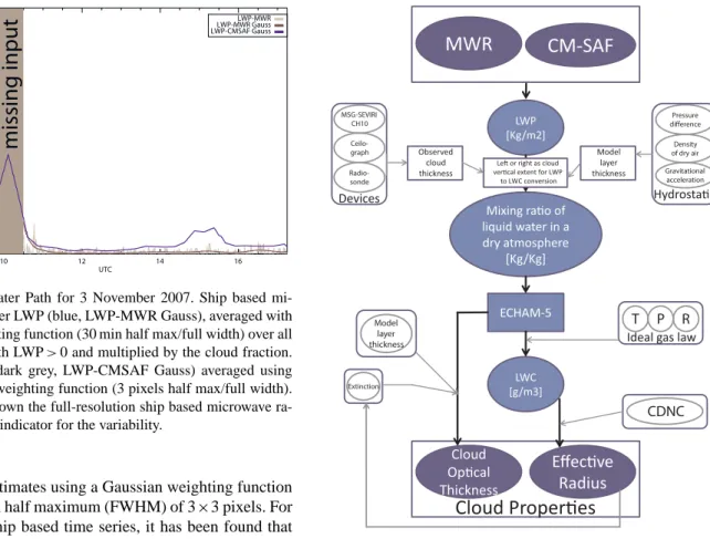
10 12 14 16 UTC 0 100 200 300 400 500 LWP [g/m 2] LWP-MWR LWP-MWR Gauss LWP-CMSAF Gauss
missing input
Fig. 1. Liquid Water Path for 3 November 2007. Ship based mi-crowave radiometer LWP (blue, LWP-MWR Gauss), averaged with a Gaussian weighting function (30 min half max/full width) over all
measurements with LWP>0 and multiplied by the cloud fraction.
CM SAF LWP (dark grey, LWP-CMSAF Gauss) averaged using spatial Gaussian weighting function (3 pixels half max/full width). In light grey is shown the full-resolution ship based microwave ra-diometer LWP as indicator for the variability.
from satellite estimates using a Gaussian weighting function with a full width half maximum (FWHM) of 3×3 pixels. For averaging the ship based time series, it has been found that Gaussian weighted averaging over 30 min leads to the best results, close to the 40 min reported by Deneke et al. (2009). This roughly corresponds to the time it takes for the ship to cross the hemispheric field of view of the pyranometer. With these averaging techniques, time series of both datasets representing similar scales of variability have been obtained. This is shown in Fig. 1 for the LWP on 3 November 2007.
4.2 Model inputs and requirements
For radiative flux calculations the optical properties of gases, aerosols and clouds are required as input to the RTM, given by the vertical profiles of extinction, single scattering albedo and the scattering phase function. From our observations, however, only the liquid water path and effective radius is available. Hence, these physical properties have to be trans-formed into consistent optical properties. For the considered shortwave range, it is known that the scattering properties of an arbitrary cloud droplet size distribution are well repre-sented by the effective radius (Hansen and Travis, 1974). In the radiative transfer scheme of GCMs the effective radius is often a diagnostic variable and a function of the liquid water path and a prescribed cloud droplet number concentration. By inverting the used relations, the effective radius can be determined for the RTM calculations. The extinction coef-ficient is again a function of the effective radius and liquid water content (LWC). The cloud optical thickness is calcu-lated internally for each spectral band from the model layer
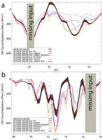
MWR
CM-SAF
Cloud Opcal ThicknessEffecve
Radius
Cloud Properes
LWP [Kg/m2] Mixing rao of liquid water in a dry atmosphere [Kg/Kg] ECHAM-5 LWC [g/m3] MSG-SEVIRI CH10 Ceilo- graph Radio- sonde Devices Pressure difference Density of dry air Gravitational acceleration Hydrostac Observed cloud thickness Model layer thicknessIdeal gas law
T P R CDNC Model layer thickness Extinction Le or right as cloud vercal extent for LWP
to LWC conversion
Fig. 2. Schematic overview on the dependences in the transforma-tion from measured liquid water path to cloud properties in the model.
thickness and the extinction coefficient. The dependencies of cloud properties in the RTM used for this study are il-lustrated in the scheme shown in Fig. 2, and formalized in the Appendix A. As mentioned before the main assumption of the RTM is the homogeneous plane parallel representa-tion of clouds. Also the cloudy column does not interact with the clear sky column. This enables modeling the cloudy at-mosphere separately from the clear and combining both by Eq. (2):
DSR=N DSRcloudy+(1−N )DSRclear (2) The linear relation uses the cloud fraction,N, to combine the modeled clear sky and cloudy irradiance. Thus, the mod-eled DSR is very sensitive to errors in cloud fraction for broken cloud situations. The used RTM can be run in two standard configurations with 19 and 31 vertical levels to re-solve a range from 1013 hPa to 10 hPa. It was chosen to lo-cate the cloud in a single model layer because cloud profile information are not available and because most clouds dur-ing the selected days have a small vertical extent. The hu-midity profiles from the radiosonde ascend are used to diag-nose the cloud base height which is used to select the closest model layer. To minimize the CPU costs the lower model
Table 1. Overview of different parameters prescribed in the model. Additionally it is shown, how these parameters are derived and what the dependencies are.
Parameter Source
Mixing ratio of calculated from LWP (ship-based
MWR or CM SAF)
liquid water and model layer thickness
calculated in two manners
CDNC (a) climatological profile from
ECHAM-5
(b) calculated from satellite effective radius based on model equations
Cloud cover calculated from total sky imager
Cloud height calculated from radiosonde
humidity profile
Temperature profile calculated from ship-based MWR
Humidity profile calculated from ship-based MWR
Surface pressure taken from the on-board
measure-ments of R/V Polarstern
resolution has been used. A fixed value for the cloud droplet number concentration is used which causes additional uncer-tainty as will be discussed in the closure study. Table 1 gives an overview of the atmospheric parameters which are input into the model including their source.
5 Closure study
For the closure study the shortwave cloud radiative ef-fect (SWCRE) at the surface has been computed with the ECHAM-5 RTM and compared to the ship-based SWCRE measurements. Six experiments have been defined for test-ing the sensitivity of the model to different combinations of ship- and satellite-based observations concerning the repre-sentation of clouds as input to the RTM. The experiments are listed below:
1. Experiment PS: the atmosphere in the model is de-scribed by ship-based measurements only. The standard profile for the cloud droplet number concentration as prescribed by ECHAM-5 is used. Hereby the effective radius is mainly a function of the measured LWP and a climatological cloud droplet number concentration. Here, PS serves as an abbreviation for Polarstern, which is the vessel ground-based measurements are perfomed on.
2. Experiment PS-RSAT: as experiment PS but with droplet effective radius, from the satellite retrieval.
Fig. 3. SWCRE for 3 November 2007 which was dominated by op-tical thin overcast conditions (a) and the SWCRE for 10 November 2007 which was dominated by broken cloud conditions with a large averaged cloud fraction (b). The grey area around the observation line refers to the standard deviation within the 30 min averaging pe-riod.
3. Experiment PS-R10: as experiment PS but with constant effective radius of 10 µm as used in the ISCCP satel-lite retrieval (i.e. Rossow and Schiffer, 1991; Han et al., 1994).
4. Experiment CMSAF: only CM SAF based LWP andre are used to describe the cloud properties.
5. Experiment CMSAF-NORSAT: as experiment CMSAF but without satellite-basedre. The ECHAM-5 standard profile of cloud droplet number concentrations is used to obtain the effective cloud droplet radius.
6. Experiment CMSAF-R10: for consistency an experi-ment using a constant effective radius of 10 µm but a LWP from the CM SAF retrieval is also included. Seven days with different atmospheric conditions have been selected for this study, ranging from clear skies to broken clouds with different cloud fraction to overcast with optically thick clouds (see Table 2). For each day the diurnal cycle of
Table 2. Top table: overview of the days used within this study with their mean location and atmospheric condition. Bottom table: daily mean
and standard deviation of cloud fraction (N) in %, liquid water path (LWP) in g m−2and cloud base height (CBH) in m.
# Date Mean position Atmospheric condition
1 31/10/2007 42◦N/10◦W Clear sky
2 02/11/2007 33◦N/13◦W Midlatitiude scattered clouds
3 03/11/2007 30◦N/14◦W Stratocumulus with break ups
4 10/11/2007 05◦N/17◦W Mixed clouds with stratocumulus fields
5 12/11/2007 02◦N/13◦W Tropical scattered clouds with clear sky periods
6 13/11/2007 01◦S/10◦W Mixed clouds with overcast periods
7 16/11/2007 10◦S/02◦W Stratocumulus with high sun
# Mean ofN STDEV ofN Mean of LWP STDEV of LWP Mean of CBH
1 3 4 2 3 479 2 15 12 24 56 561 3 75 23 23 51 1860 4 54 24 64 17 2554 5 10 8 20 32 1461 6 67 29 48 90 828 7 74 31 32 29 1207
the surface SWCRE has been modeled with a temporal res-olution of 15 min corresponding to the SEVIRI repeat cycle. Equation (3) defines the SWCRE at the surface as used here, withαdenoting the ocean albedo taken from ECHAM-5. SWCRE=(1−α)(DSRall sky−DSRclear) (3) Figure 3 shows the diurnal cycle of the SWCRE for two days. The upper panel displays a day nearly overcast clouds which are breaking up during noon and which are getting thinner in the afternoon. The lower panel displays a day with broken clouds dominated by a large cloud fraction. In both panels the black curve corresponds to the ship based measurements and the shaded area around it covers±one standard deviation for each averaging period. The other curves show the mod-eled SWCRE for the different experiments (blue for exper-iment PS, light blue for experexper-iment PS-RSAT, magenta for experiment PS-R10, red for experiment CMSAF, orange for experiment CMSAF-NORSAT, and brown for experiment CMSAF-R10). The light grey bar is used to indicate prob-lems with the input data such as rain for the microwave ra-diometer, sunglint for CM SAF data, shadowing of the pyra-nometer, etc. Both panels indicate that the model can roughly reproduce the diurnal cycle of the SWCRE. There is a signif-icant spread within the six experiments as well as a more or less pronounced bias compared to the observed SWCRE.
The low-level mostly cloudy cloud situation in Fig. 3a un-til 12:00 UTC is well captured by most experiments. This also indicates that the additional satellite-based information of cloud droplet effective radius improves the representation of the state of the atmosphere. As the sky slightly clears during noon, a pronounced broken cloud effect (positive SWCRE) occurs, which cannot be reproduced by the RTM leading to a strong underestimation. In the afternoon, the
ex-periments show the largest variability and generally underes-timate the SWCRE, i.e. they produce smaller cloud-induced shading than is shown in the observations. Interestingly, the experiments with satellite-based LWP show better results in-dicating that the ship-based microwave radiometer underesti-mates the LWP for the thinner water clouds in the afternoon. The strongly inhomogeneous broken cloud case in Fig. 3b shows a correspondingly large variability in the observed SWCRE that is partly captured by the six model experiments. Again, all RTM results show a similar deviation from the ob-servation due to the inherent cloud homogeneity that can not reproduce situations with local clouds blocking the direct so-lar irradiation or cloud holes that allow for direct sun despite a large cloud fraction. Both situations explain the systematic biases around 13:00, 14:00 and 15:00 UTC. There is no sin-gle combination of ship- and satellite-based cloud descrip-tion that explains the observadescrip-tions best. At least, ship-based LWP with satelliterework better than using ship-based mea-surements only.
Finally, the ability of the different RTM experiments to re-produce the downwelling shortwave radiation has been quan-tified and compared. In Table 3, the differences between the modeled and the measured (model−measurement) daily mean DSR, the bias, are shown in W m−2. In the second col-umn of the table, the daily mean measured DSR is shown, which are the pyranometer measurements with times of shad-owing through ship superstructures removed. In the third col-umn the clear sky mean DSR is shown. The parametrisation from Kalisch and Macke (2008) is used to calculate the DSR for this purpose under clear conditions. For the clear sky case a slightly larger DSR is observed, compared to the modeled clear sky value. This deviation is most likely the result of two competing effects: the shadowing of the forward scattered
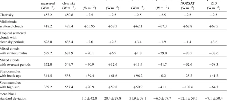
Table 3. Results of the six experiments applied to seven different atmospheric conditions examined within this study are shown as deviations of the modeled to the measured daily mean DSR(bias). Additionally the measured and parameterized clear sky DSR at the surface is given
in W m−2. The parametrization is taken from Kalisch and Macke (2008). In the last two rows the mean bias and the mean absolute deviation
of the bias over all cases and for each experiment is shown in W m−2.
Mean DSR Mean DSR Exp. PS Exp. PS-RSAT Exp. PS-R10 Exp. CMSAF Exp. CMSAF- Exp.
CMSAF-measured clear sky NORSAT R10
(W m−2) (W m−2) (W m−2) (W m−2) (W m−2) (W m−2) (W m−2) (W m−2) Clear sky 453.2 450.8 −2.5 −2.5 −2.5 −2.5 −2.5 −2.5 Midlatitude scattered clouds 418.2 495.4 +55.95 +58.3 +62.1 +67.3 +62.8 +69.5 Tropical scattered clouds with
clear sky periods 628.0 638.4 −2.0 +2.3 +3.4 +1.9 −1.4 +3.6
Mixed clouds
with stratocumulus 529.2 682.9 −70.1 +6.9 +1.8 −29.0 −93.5 −38.6
Mixed clouds
with overcast periods 352.0 549.7 −30.9 +12.6 +11.4 −41.7 −62.6 −58.3
Stratocumulus
with break ups 341.5 535.1 +39.4 +61.6 +96.2 −0.2 −25.2 +41.2
Stratocumulus
with high sun 389.2 557.4 +20.9 +59.8 +50.9 −41.1 −102.6 −64.7
mean bias±
standard deviation 1.5±42.8 28.4±29.8 31.9±38.1 −6.5±37.7 −32.1±58.5 −7.1±50.4 mean absolute deviation
of the bias 31.7 29.1 32.6 26.2 50.1 39.8
solar radiation and the reflection of solar radiation by the ship’s superstructure. The observed diurnal cycle of the clear sky flux (not shown here) indicates that the reflection effect is slightly stronger than the shadowing effect. However, the difference between the two artifacts is less than 3 W m−2, which is well within the accuracy of the pyranometer. Dif-ferent aerosol loads can also be the source of the deviation. The small deviation for the clear sky case shows that in the absence of clouds the RTM can well reproduce the diurnal cycle of DSR at the surface.
Summarizing the results in Table 3, no clear quality differ-ences are found between using ship-based or satellite-based cloud properties for describing the observed short wave cloud radiative effect. Compared to Ebell et al. (2011) for most ex-periments a lower bias is found when considering the mean absolute deviation of the bias of each experiment over all cases. Both experiment groups, CMSAF and PS, show sim-ilar values which decrease when the satellite based effective radius is included in the dataset. Furthermore, we compared our findings to the CM SAF target accuracies in their CDOP Product Requirments Document CMSAF (2011), which specifies 20 W m−2 for daily means as target accuracy for the surface incoming shortwave radiation product. Applied to our results for mean bias, the 20 W m−2can be achieved for three of the six experiments. Compared to the mean ab-solute deviation of the bias of our results the 20 W m−2 is smaller, but both experiments which include the CM-SAF
effective Radius achieve accuracies relatively close to this target (26 W m−2and 29 W m−2). Results of the single cases show that the experiments CMSAF show better results for the overcast case with optically thin clouds and also for the broken cloud case with large cloud fraction. Experiment PS shows slightly better results for the broken cloud case with small cloud fraction. These results are possibly related to the fact that satellite retrievals of cloud properties have more problems with small-scale cloudiness than surface-based re-trieval schemes. Using the effective radius as additional in-formation for the experiments CMSAF and PS leads to the same or better results compared to the experiments with the standard CDNC profile and the constant effective radius. Re-sults of both experiments using a constant effective radius do show deviations similar or larger compared to the exper-iments with the prescribed CM SAF effective radius under nearly all conditions.
Comparing our results under clear sky conditions to those of Guo and Coakley (2008) slightly smaller deviations are found in our comparison between modeled and measured DSR. For a clear sky day an average difference of about 0.5 % has been found. Guo and Coakley (2008) compared the surface radiation measured on board of a vessel to model results. Their model was driven by atmospheric profiles from NCEP analysis fields. They found an averaged disagreement of 2 % over 12 days selected for constant clear sky condi-tions. However, given the larger measurement uncertainties
and only a single day of data for our study, this difference is not statistically significant. Generally, a larger number of cases should be considered to obtain statistically robust esti-mates of the model performance under the different synopti-cal situations.
Another study comparing ship-based measured DSR and satellite based estimates of DSR is Macke et al. (2010b). They compared instantaneous and daily data and determined random and systematic deviations. Our results for daily mean DSR show higher deviations (up to 102 W m−2versus 20 W m−2 in Macke et al., 2010b). This likely results from the additional complexity introduced by using the ship-based cloud properties, with their specific uncertainties and yet an-other sampling geometry.
There are several problems and limitations which are re-sponsible for the quality of the modeled SWCRE. Firstly, the timeseries of MWR-LWP only samples a one-dimensional cross section of the area of interest. Thus, any anisotropy in the horizontal LWP distribution will result in a sampling bias compared to a 2-D LWP sampling as performed by the lite retrievals. Sub-pixel inhomogeneity also biases the satel-lite retrieval towards smaller LWP. Related to this problem, the specific cloud constellation relative to the sun position is relevant, which cannot be resolved from the satellite ob-servations but has a strong effect on the CRE, i.e. by block-ing or passblock-ing the direct solar irradiation. Furthermore, the cloud cover used in this study is derived from the sky imager for pixels with a wide range of observation zenith angles. Hence, it may be biased relative to zenith view for broken clouds with large vertical extent due to obscuration by cloud sides and is affected by clouds which have little relevance for radiation e.g. opposite to the sun and far away at the hori-zon. These problems limit the ability of performing a 1-D radiative closure study from ground- and satellite based ob-servations.
6 Summary and conclusion
This study addresses the following two questions: (1) How accurate does the radiative transfer scheme of the ECHAM-5 GCM reproduce the measured SWCRE over the ocean based on ship-based and satellite-based estimates of the at-mospheric state? (2) Is there an optimal combination of ship-and satellite-based observation that describes the SWCRE best? To answer these questions, modeled SWCRE have been compared to SWCRE from ship observations.
For this purpose six different experiments have been con-ducted, and their results have been analyzed for results for seven different atmospheric conditions. The experiments dif-fer in the way the parameter used to describe the clouds are coming from, either from ship-based or satellite measure-ments alone, from a combination of both or from a combi-nation of measurements and a-priori cloud properties.
In the considered cases, using satellite data does not result in a loss in accuracy. Furthermore, we could not identify a higher accuracy by using the ship-based cloud properties as model input. Satellite estimates can show reduced accuracies under broken cloud situations with small cloud fraction. This is likely due to sub-pixel cloudiness that is not resolved by the satellite. For the numerical experiments an improvement by using the satellite-based estimate of effective radius as additional input to the ship-based observations mostly has been found.
The strong variability of the DSR in broken cloud situa-tions causes a fundamental problem in the comparison of ra-diative transfer model results and radiation measurements. To overcome this issue models which include three dimensional radiative transfer effects are needed together with realistic cloud fields. In addition, we have to deal with the problem of merging two different observations, from the surface and the top of atmosphere, which leads to systematic uncertain-ties. Additional instruments such as a cloud radar, as it will be available on research vessels in the future, combined with a increased set of data can reduce the limitations which were encountered in this study. An interesting aspect would be the closure of satellite based estimates and ship data in overcast conditions compared to broken cloudy conditions. Unfortu-nately, in our dataset no fully overcast day could be found.
This study also demonstrates the importance of using the pixel-based level-2 CM SAF data for studying deviations be-tween modeled and measured irradiance. In several cases, mechanisms responsible for the differences between mod-eled radiation and the pyranometer measurements could only be analyzed because of the high temporal and spatial resolu-tion of the level-2 data.
Appendix A
Relationship between cloud physical and optical properties
For calculating the radiative effects of a cloud by means of a radiative transfer model, the vertical profile of cloud optical properties are required as input (extinction, single scattering albedo, phase function). Atmospheric models and measure-ments, however, often provide information about clouds in form of physical parameters such as cloud water content or cloud droplet size/size distribution. Hence, the relationships between the physical and optical properties have to be es-tablished. In this appendix, we present a short overview of the most important relations for our study. Our discussion is based on Liou (1980).
The spatial distribution of cloud droplets is completely de-scribed by the spectral cloud droplet size distribution,n(r).
For many applications, the total cloud droplet number con-centration,N, is of interest, which is given by
N=
∞
Z
0
n(r)dr . (A1)
Using some basic mathematics, we can derive the main phys-ical cloud properties from the size distribution:
– The liquid water content is given by
LWC=4 3πρw ∞ Z 0 r3n(r) dr , (A2)
withρw as the density of liquid water, and 43π as vol-ume of one cloud droplet assuming a spherical particle shape.
– The extinction coefficient is defined by
βext=π
∞
Z
0
Qext(r)r2n(r) dr , n(r)dr , (A3)
whereQextπ r2denotes the extinction cross section of an individual cloud droplet.Qextis called the extinction efficiency factor, and is a function of the cloud droplet radius, the wavelengths of the stimulating light beam, and the refraction index. The extinction efficiency fac-tor for cloud droplets can be set to 2 (Liou, 1980; Hu and Stamnes, 1993) with good accuracy in the visible wavelength range.
– Both relations can be re-written usingN: LWC=4
3N πρwr 3
vol, (A4)
withrvol ˆ=, volume mean radius
βext=N π Qextra2=2N π ra2, (A5) withra2ˆ=cross sectional area
Hu and Stamnes (1993) show that cloud optical properties, as they are used in radiative transfer models, are mainly sensi-tive to the effecsensi-tive radiusre, which is defined by the ratio of the second and third moment of the droplet size distribution n(r): re= R∞ 0 r 3n(r) dr R∞ 0 r2n(r) dr =r 3 vol r2 a . (A6)
To account for the differences betweenrvol, that we can ob-tain from the cloud water concentration, andre, that repre-sents the size distribution for scattering purposes, a conver-sion factorkis introduced:re=krvol. Roeckner et al. (2003) determined the value ofkas 1.077 for maritime clouds.
On a closer look we identify in Eq. (A2) the 3rd moment of the cloud droplet size distribution and in the Eq. (A3) the 2nd moment. Substituting the 3rd moment from Eq. (A2) and and 2nd moment from Eq. (A3) into Eq. (A6), the following well known (i.e. Reid et al., 1999) relation is obtained: re=3 4 2π πρw LWC βext =3 2 LW C βext (A7) In our study, the measurements do not provide the extinc-tion coefficient. Therefore, we need relaextinc-tion Eq. (A7) in an-other form. We can derive an expression ofredirectly from Eq. (A2).rvol=q3 3LWC
4πρwN still consists the volume radius and
we have to use the conversionre=krvoland derive: re=k3
s LW C 4πρwN
. (A8)
With a detailed look the difference between Eqs. (A7) and (A8) is the extinction coefficient, which is replaced by its definition. For the purpose of our study, functions containing extinction and liquid water content can be integrated verti-cally over the atmospheric column by assuming a vertiverti-cally homogeneous cloud layer and transforming them to the LWP and COT as function parameters. This also enables solving Eq. (A7) for the COT.
Acknowledgements. This work was supported financially by the
CM SAF consortium and EUMETSAT through a visiting scientist activity. We are grateful to Daniel Klocke from MPI Hamburg for providing the Single Column Model and Sebastian Wahl for giving technical support with the model. Furthermore, we thank John Kalisch and Yann Zoll for providing TSI and MWR data as well as for providing algorithms for cloud cover and LWP calculations. We are grateful to the Alfred-Wegener-Institute for the opportunity to perform measurements during the Atlantic transfer cruises of R/V POLARSTERN. We are also grateful to the crew of R/V
POLARSTERN for valuable support in the organization and
perfor-mance on all our cruises, in this case especially ANT-XXIV/1. Edited by: Q. Fu
References
Althausen, D., Engelmann, R., Baars, H., Heese, B., Ans-mann, A., Mueller, D., and Komppula, M.: Portable Raman Lidar Polly(XT) for automated profiling of aerosol backscatter, extinc-tion, and depolarizaextinc-tion, J. Atmos. Ocean. Tech., 26, 2366–2378, 10.1175/2009JTECHA1304.1, 2009.
Barkstrom, B. R.: The Earth Radiation Budget Experiment (ERBE), Bull. Amer. Meteor. Soc., 65, 1170–1185,
doi:10.1175/1520-0477(1984)065<1170:TERBE>2.0.CO;2, 1984.
Bedacht, E., Gulev, S. K., and Macke, A.: Intercomparison of global cloud cover fields over oceans from the VOS observations and NCEP/NCAR reanalysis, Int. J. Climatol., 27, 1707–1719, doi:10.1002/joc.1490, 2007.
Clough, S., Shephard, M., Mlawer, E., Delamere, J., Ia-cono, M., Cady-Pereira, K., Boukabara, S., and Brown, P.: Atmospheric radiative transfer modeling: a summary of the AER codes, J. Quant. Spectrosc. Ra., 91, 233–244, doi:10.1016/j.jqsrt.2004.05.058, 2005.
CMSAF Technical Team: CDOP Product Requirements Document, SAF on climate monitoring, Doc. No.: SAF/CM/DWD/PRD/1, Issue: 1.8, Date: 22 November 2011, 2011.
Crewell, S. and Loehnert, U.: Accuracy of cloud liquid water path from ground-based microwave radiometry – 2. sensor accuracy and synergy, Radio Sci., 38, 8042, doi:10.1029/2002RS002634, 2003.
Deneke, H. M., Feijt, A., van Lammeren, A., and Simmer, C.: Val-idation of a physical retrieval scheme of solar surface irradi-ances from narrowband satellite radiirradi-ances, J. Appl. Meteorol., 44, 1453–1466, doi:10.1175/JAM2290.1, 2005.
Deneke, H. M., Knap, W. H., and Simmer, C.: Multiresolution anal-ysis of the temporal variance and correlation of transmittance and reflectance of an atmospheric column, J. Geophys. Res., 114, D17206, doi:10.1029/2008JD011680, 2009.
Ebell, K., Crewell, S., Loehnert, U., Turner, D. D., and O’Connor, E. J.: Cloud statistics and cloud radiative effect for a low-mountain site, Q. J. Roy. Meteor. Soc., 137, 306–324, doi:10.1002/qj.748, 2011.
Greuell, W. and Roebeling, R. A.: Toward a standard procedure for validation of satellite-derived cloud liquid water path: a study with SEVIRI data, J. Appl. Meteorol. Clim., 48, 1575–1590, doi:10.1175/2009JAMC2112.1, 2009.
Guo, G. and Coakley, J. J. A.: Satellite estimates and shipboard observations of downward radiative fluxes at the ocean surface, J. Atmos. Ocean. Tech., 25, 429–441, doi:10.1175/2007JTECHA990.1, 2008.
Han, Q., Rossow, W., and Lacis, A.: Near-global survey of effective droplet radii in liquid water clouds using ISCCP data, J. Climate, 7, 465–497,
doi:10.1175/1520-0442(1994)007<0465:NGSOED>2.0.CO;2, 1994.
Hansen, J. and Travis, L.: Light scattering in planetary atmospheres, Space Sci. Rev., 16, 527–610, doi:10.1007/BF00168069, 1974. Hu, Y. and Stamnes, K.: An accurate parameterization of
the radiative properties of water clouds suitable for use in climate models, J. Climate, 6, 728–742,
doi:10.1175/1520-0442(1993)006<0728:AAPOTR>2.0.CO;2, 1993.
IPCC, 2007: Summary for Policymakers, in: Climate Change 2007: The Physical Science Basis. Contribution of Working Group I to the Fourth Assessment Report of the Intergovernmental Panel on Climate Change, edited by: Solomon, S., Qin, D., Manning, M., Chen, Z., Marquis, M., Averyt, K. B., Tignor, M., and Miller, H. L., Cambridge University Press, Cambridge, UK and New York, NY, USA.
Kalisch, J. and Macke, A.: Estimation of the total cloud cover with high temporal resolution and parametrization of short-term fluc-tuations of sea surface insolation, Meteorol. Z., 17, 603–611, 2008.
Kalisch, J. and Macke, A.: Radiative budget and cloud radiative effect over the Atlantic from ship based observations, Atmos. Meas. Tech.,5, 2391-2401, doi:10.5194/amt-5-2391-2012, 2012. Kipp and Zonen: Instruction Manual CM 21. – Manual Version: 0904, Kipp & Zonen B. V., Delftechpark 36, 2628 Delft, The Netherlands, 2004.
Koepke, P., Hess, M., Schult, I., and Shettle, E.: Global Aerosol Data Set, MPI Rep. 243, Max-Planck-Institut f¨ur Meteorologie, Hamburg, Germany, 44 pp., 1997.
Liou, K.: An Introduction to Atmospheric Radiation, Academic Press, New York, USA, 136–139, 1980.
Macke, A.: The Expedition of the Research Vessel “Polarstern” to the Antarctic in 2008 (ANT-XXIV/4), in: Berichte zur Polar-und Meeresforschung – Reports on Polar and Marine Research, edited by Macke, A., 591, Alfred-Wegener-Institut, Bremer-haven, 65 pp., 2009.
Macke, A., Kalisch, J., Sinitsyn, A., and Wassmann, A.: More of MORE: the first MORE cruise onboard RV Polarstern, WGSF/WCRP Flux News, 21–22, 2007.
Macke, A., Kalisch, J., Zoll, Y., and Bumke, K.: Radiative effects of the cloudy atmosphere from ground and satellite based obser-vations, EPJ Web of Conferences, 9, 83–94, 2010a.
Macke, A., Kalisch, J., and Hollmann, R.: Validation of down-ward surface radiation derived from MSG data by in-situ ob-servations over the Atlantic ocean, Meteorol. Z., 19, 155–167, doi:10.1127/0941-2948/2010/0433, 2010b.
Ramanathan, V., Cess, R., Harrison, E., Minnis, P., Barkstrom, B., Ahmad, E., and Hartmann, D.: Cloud-radiative forcing and cli-mate: results from the earth radiation budget experiment, Sci-ence, 243, 57–63, doi:10.1126/science.243.4887.57, 1989. Reid, J., Hobbs, P., Rangno, A., and Hegg, D.: Relationships
between cloud droplet effective radius, liquid water content, and droplet concentration for warm clouds in Brazil embedded in biomass smoke, J. Geophys. Res.-Atmos., 104, 6145–6153, doi:10.1029/1998JD200119, 1999.
Roebeling, R. A., Feijt, A. J., and Stammes, P.: Cloud property re-trievals for climate monitoring: implications of differences be-tween spinning enhanced visible and infrared imager (SEVIRI) on METEOSAT-8 and advanced very high resolution radiome-ter (AVHRR) on NOAA-17, J. Geophys. Res., 111, D20210, doi:10.1029/2005JD006990, 2006.
Roebeling, R. A., Deneke, H. M., and Feijt, A. J.: Validation of cloud liquid water path retrievals from SEVIRI using one year of CloudNET observations, J. Appl. Meteorol. Clim., 47, 206–222, doi:10.1175/2007JAMC1661.1, 2008.
Roeckner, E., B¨auml, G., Bonaventura, L., Brokopf, R., Esch, M., Giorgetta, M., Hagemann, S., Kirchner, I., Kornblueh, L., Manzini, E., Rhodin, A., Schlese, U., Schulzweida, U., and Tomkins, A.: The Atmospheric General Circulation Model ECHAM5: part I: Model description, MPI Rep. 349, Max-Planck-Institut f¨ur Meteorologie, Hamburg, Germany, 127 pp., 2003.
Rose, T., Crewell, S., Loehnert, U., and Simmer, C.: A network suitable microwave radiometer for operational monitoring of the cloudy atmosphere, Atmos. Res., 75, 183–200, 2005.
Rossow, W. and Schiffer, R.: ISCCP cloud data products,
B. Am. Meteorol. Soc., 72, 2–20,
doi:10.1175/1520-0477(1991)072<0002:ICDP>2.0.CO;2, 1991.
Schulz, J. and Hollmann, R.: Climate Monitoring
SAF Annual Product Quality Assessment, CM SAF,
SAF/CM/DWD/VAL/OR5, 2009.
Schulz, J., Albert, P., Behr, H.-D., Caprion, D., Deneke, H., Dewitte, S., D¨urr, B., Fuchs, P., Gratzki, A., Hechler, P., Hollmann, R., Johnston, S., Karlsson, K.-G., Manninen, T., M¨uller, R., Reuter, M., Riihel¨a, A., Roebeling, R.,
Sel-bach, N., Tetzlaff, A., Thomas, W., Werscheck, M., Wolters, E., and Zelenka, A.: Operational climate monitoring from space: the EUMETSAT Satellite Application Facility on Climate Monitoring (CM-SAF), Atmos. Chem. Phys., 9, 1687–1709, doi:10.5194/acp-9-1687-2009, 2009.
Sinitsyn, A., Gulev, S., Macke, A., Kalisch, J., and Sokov, A.: MORE cruises launched, WGSF/WCRP Flux News, 11–13, 2006.
Smirnov, A., Holben, B. N., Slutsker, I., Giles, D. M., Mc-Clain, C. R., Eck, T. F., Sakerin, S. M., Macke, A., Croot, P., Zibordi, G., Quinn, P. K., Sciare, J., Kinne, S., Harvey, M., Smyth, T. J., Piketh, S., Zielinski, T., Proshutinsky, A., Goes, J. I., Nelson, N. B., Larouche, P., Radionov, V. F., Goloub, P., Moor-thy, K. K., Matarrese, R., Robertson, E. J., and Jourdin, F.: Mar-itime aerosol network as a component of aerosol robotic network, J. Geophys. Res., 114, D06204, doi:10.1029/2008JD011257, 2009.
Turner, D. D., Vogelmann, A. M., Austin, R. T., Barnard, J. C., Cady-Pereira, K., Chiu, J. C., Clough, S. A., Flynn, C., Khaiyer, M. M., Liljegren, J., Johnson, K., Lin, B., Long, C., Marshak, A., Matrosov, S. Y., McFarlane, S. A., Miller, M., Min, Q., Minnis, F., O’Hirok, W., Wang, Z., and Wiscombe, W.: Thin liquid water clouds: their importance and our challenge, B. Am. Meteorol. Soc., 88, 177–190, doi:10.1175/BAMS-88-2-177, 2007.
Wielicki, B. A.,Barkstrom, B. R.,Harrison, E. F.,Lee, R. B., Smith, G. L., Cooper, J. E.: Clouds and the earth’s radiant energy system (CERES): An earth observing system experi-ment, B. Am. Meteorol. Soc.,77, 853–868,
doi:10.1175/1520-0477(1996)077<0853:CATERE>2.0.CO;2, 1996.
World Meteorological Organization: Guide to Meteorological In-struments and Methods of Observations, WMO-NO 8, 2008. Wulfmeyer, V., Behrendt, A., Kottmeier, C., Corsmeier, U.,
Barthlott, C., Craig, G. C., Hagen, M., Althausen, D., Aoshima, F., Arpagaus, M., Bauer, H.-S., Bennett, L., Blyth, A., Brandau, C., Champollion, C., Crewell, S., Dick, G., Di Giro-lamo, P., Dorninger, M., Dufournet, Y., Eigenmann, R., Engel-mann, R., Flamant, C., Foken, T., Gorgas, T., Grzeschik, M., Handwerker, J., Hauck, C., H¨oller, H., Junkermann, W., Kalthoff, N., Kiemle, C., Klink, S., K¨onig, M., Krauss, L., Long, C. N., Madonna, F., Mobbs, S., Neininger, B., Pal, S., Peters, G., Pigeon, G., Richard, E., Rotach, M. W., Russchen-berg, H., Schwitalla, T., Smith, V., Steinacker, R., Trentmann, J., Turner, D. D., van Baelen, J., Vogt, S., Volkert, H., Weckw-erth, T., Wernli, H., Wieser, A., and Wirth, M.: The convective and orographically-induced precipitation study (COPS): the sci-entific strategy, the field phase, and research highlights, Q. J. Roy. Meteor. Soc., 137, 3–30, doi:10.1002/qj.752, 2011.