Kashfi, Syeed,
Bunker, Jonathan M., &
Yigitcanlar, Tan
(2015)
Effects of transit quality of service characteristics on daily bus ridership. In
Perk, Victoria (Ed.)
Transportation Research Board 94th Annual Meeting Compendium of
Pa-pers, Transportation Research Board of the National Academies,
Wash-ington, D.C.
This file was downloaded from:
http://eprints.qut.edu.au/80275/
c
Copyright 2015 The Authors
Notice
:
Changes introduced as a result of publishing processes such as
copy-editing and formatting may not be reflected in this document. For a
definitive version of this work, please refer to the published source:
Name: Syeed Anta Kashfi (Corresponding author)
3
Affiliation: School of Civil Engineering and Built Environment
4
Address: 2 George Street, GPO Box 2434, Brisbane QLD 4001, Australia
5
6
7
8
9
Name: Associate Professor Jonathan M Bunker
10
Affiliation: School of Civil Engineering and Built Environment
11
Address: 2 George Street, GPO Box 2434, Brisbane QLD 4001, Australia
12
13
14
15
Name: Associate Professor Tan Yigitcanlar
16
Affiliation: School of Civil Engineering and Built Environment
17
Address: 2 George Street, GPO Box 2434, Brisbane QLD 4001, Australia
18
19
20
21
22
23
Word Count Abstract (Limit 250) 176All Text (excludes reference) 5,381
3 tables + 2 figure 1,250
Total 6,807
Number of references 35
24
25
Submitted for Publication and Presentation
26
Submission date: July 31, 2014
27
28
29
ABSTRACT
1
This study explores how explicit transit quality of services (TQoS) measures including service frequency, service
2
span, and travel time ratio, along with implicit environmental predictors such as grade factor influence bus ridership
3
using a case study city of Brisbane, Australia. The primary hypothesis tested was that bus ridership is higher within
4
suburbs with high transit quality of service than suburbs that have limited service quality. Using Multiple Linear
5
Regression (MLR) this study identifies a strong positive relationship between route intensity (bus-km/h-km2) and
6
bus ridership, indicating that increasing both service frequency and spatial route density correspond to higher bus
7
ridership. Additionally, travel time ratio (in-vehicle transit travel time to in-vehicle auto travel time) is also found to
8
have significant negative association with ridership within a suburb, reflecting a decline in transit use with increased
9
travel time ratio. Conversely, grade factor and service span is not found to exert any significant impact on bus
10
ridership in a suburb. Our study findings enhance the fundamental understanding of traveller behaviour which is
11
informative to urban transportation policy, planning and provision.
12
13
14
15
Keywords: Frequency, Route Density, Travel Time, Transit, Quality of Service, Grade, Bus
16
INTRODUCTION
1
Public transport provides basic mobility services to people in their day to day activities. It helps to reduce road
2
congestion, travel times, air pollution, and energy consumption compared to other travel modes. However, despite
3
its benefits, a large proportion of the traveling public is reluctant to use transit as their preferred mode of travel. A
4
host of factors related to transit ridership are either directly or indirectly responsible for this. This includes
socio-5
economic characteristics of trip makers such as car ownership, driver’s licence availability, age, gender, race,
6
ethnicity, employment status, and occupation type, as well as household socio-economic characteristics, such as
7
household size, household structure and composition, housing tenure, lifestyle, and attitude towards using transit (
1-8
3). Geographic elements such as walkability, parking availability, and parking cost at origin and destination also
9
influence transit ridership(3).Despite all of these factors being known, the effects of Transit Quality of Service
10
(TQoS) measures (4) on actual transit ridership on a daily basis has received limited attention in the literaturefor
11
Brisbane, capital of Queensland state, Australia. One exception was a study by Muley et al. (5) focusing on a transit
12
supportive suburb of Kelvin Grove in this region.
13
Brisbane comprises sprawling land use patterns and a largely auto-oriented transport system, dominated by
14
large arterial roads, freeways and tollways. However, the city is also well served by three integrated transit modes;
15
bus, heavy rail, and linear ferry. Bus ridership is higher than rail and substantially higher than ferry. Bus is heavily
16
reliant on a busway (BRT) network of four lines spanning more than 25km (16 mi), which are fed by more than half
17
of the city’s routes, and which offer strong connections to the heavy rail network. It comprises a mixture of
grade-18
separated bus-only sections with on-street transitway sections, complementing the region's urban rail network to
19
provide faster and more efficient bus services to its residents (6). The maximum load segment (MLS) on Brisbane’s
20
South East Bus way carries over 11,000 p/h during the a.m. peak (7), which equates to approximately five to six
21
busy motorway lanes.In Brisbane city, approximately 43,707 people use bus for their main daily travel while 26,840
22
people use train (8). Since bus is the city’s dominant transit mode, factors that affect its ridership are worthy of
23
investigation.
24
The paper focuses on transit ridership, because conceivably it is the single most important dimension of
25
transit system performance.Transit systems devoid of riders does not improve social welfare. Absence of transit
26
quality of service might discourage passengers to access transit services, even when a transit stop is located within a
27
reasonable terrain and walking distance of one’s origin and destination with full walking amenities. Therefore, the
28
main purpose of this study is to assess the hypothesis that suburbs having high transit quality of service are
29
associated with higher transit ridershipcompared with suburbs having low transit quality of service.
30
Typically, access to transit stop/station can be made in number of ways including walking, bicycling, auto
31
drop-off and auto park-and-ride (4). Walking dominates, so is considered as one of the major facets of transit
32
ridership (9). However, numerous barriers to walking exist including several environmental factors such as
33
topography (10). Brisbane is a hilly city. It is often presumed that topography negatively affects transit users as they
34
access the transit stop, such that hilly suburbs ought to be less conductive to transit ridership than flat suburbs. To
35
better understand the effect of a suburb’s hilliness on daily ridership, grade factor will be considered in this study.
36
The first section of this paper provides a detailed literature review of effects of transit service provision on
37
ridership in terms of two principle sets of measures; availability, and comfort and convenience. The next section
38
provide a description of research study area. The third section categorizes the sources of data sets used in this study.
39
It also describes adjustments made to ridership data as well as other variables. The fourth section develops two sets
40
of models and presents and interprets estimation results. The final section concludes the analysis and proposes
41
further research, and provides recommendations for transit agencies, transport planners and policy makers.
42
PREVIOUS STUDIES
43
Numerous studies have examined how travel behaviour or ridership changes depending on various dimensions of
44
urban form. Most studies have concluded that high-density and mixed use developments with good pedestrian
45
environment are associated with higher transit use (2, 3, 11-13). Similarly, a number of studies have explored how
46
built environment variables can be associated with physical activity and public health (14-16). However, compared
47
to these studies, few have explored how transit quality of services affects patronage. This paper helps to overcome
48
this knowledge gap. It is perceived that people only choose transit over private vehicle when transit effectively
competes in terms of its service frequency, service span, coverage, reliability, speed, convenience, and comfort. The
1
Transit Capacity and Quality of Service Manual (TCQSM) holds detailed explanation and calculation method for all
2
transit service variables (4). TCQSM groups the Transit Quality of Services(TQoS) indicators for fixed-route transit
3
services into two principal sets, Availability and Comfort and Convenience. Usually, availability is measured by
4
Frequency, Service Span and Access and Comfort and Convenience by reliability, travel time and passenger load.
5
This section reviews the literature on transit service availability, and some aspects of comfort and convenience.
6
Availability
7
Previous research identified a significant impact of service availability (frequency and service coverage) on transit
8
ridership. Those studies confirm that the influence of transit service on ridership is relatively greater than that of
9
transit fares (17, 18). By holding all other factors constant, if service frequency is increased, demand for transit must
10
increase (19). Moreover, it is argued that when transit service is not adequate, land use qualities never provide
11
sufficient impact to shift mode share to transit, even if land use position is optimal (3). Littman argues that
12
increasing service frequency reduces the wait time of traveller’s and thus increases the demand for transit service
13
(19). In order to attract sufficient ridership, sufficient services need be available both in peak hours and off-peak
14
hours throughout the week. A positive relationship among service span and bus passengers was revealed using the
15
Canadian Urban Transit database by the means of multiple regression method (20).
16
Likewise route density, or vehicle miles of service in an area, has been used as a service availability
17
measure. According to TCQSM, this variable is labelled under the category of access or service coverage. Studies
18
have confirmed a significant positive association between route density and transit ridership (17, 18). Hendricks’s
19
study also looked at the effect of service coverage and identified that greater service coverage across the region
20
leads to greater potential ridership (3). Notwithstanding, it is not necessarily feasible to mitigate commuters’ wait
21
time by just increasing service frequency or service span, as it will increase the operating cost and could contribute
22
to road system congestion (21). Few studies have also looked at alternative means of increasing quality of service.
23
Comfort and Convenience
24
Transit quality of service is considered by some researchers to be a more important factor to attract ridership than
25
decreases in fare or increase in quantity of service (22, 23). These studies argue that riders are more concerned about
26
service quality improvement (such as live schedule information, on-street service, station/stop safety, customer
27
service, and cleanliness) than reduced fare. Concurring with these findings a number of studies suggest that transit
28
information must be available when using transit service (24, 25). Even though provision of real-time route
29
information can be costly, providing it at stations while waiting for transit can be a useful mechanism to minimize
30
perceptions of uncertain arrival times. An inverse link between available information and perceived wait time was
31
found in Dublin, Ireland (24). A California study explored that passengers are more likely to use transit services if
32
certain information is provided (25). These studies all conclude that investment in real time information is not
33
insignificant. Further, access to real time transit information through smartphone applications and
smartphone-34
friendly websites is becoming ubiquitous.
35
While providing real time information to transit riders is becoming essential, travel time remains critical.
36
TCQSM (4) mentions travel time as “an important factor in a potential transit user's decision to use transit on a
37
regular basis”. Thompson et al. (26) divided transit travel time into four different components; walk time to and
38
from transit service, wait time for initial transit vehicle, transfer time, and in-vehicle travel time. Commonly people
39
perceive transit travel time as how much longer the trip will take in comparison with automobile. In order to attract
40
transit ridership, total transit travel time should be competitive with car travel time. Usually, transit services must
41
observe multiple stops, so transit priority treatments are important as a counteracting measure. Faster speeds can be
42
achieved by providing dedicated path network (3) or guideway. Examples for bus include segregated BRT,
43
dedicated on-street bus lane, and high occupancy vehicle lane. An excellent example of reducing service gap
44
between transit and private automobiles is the grade-separated busway network in Brisbane. Another method of
45
decreasing travel time between origin and destination is by direct routing. Passengers value shorter travel times that
46
offer more direct routing (3). Obtaining direct connections with minimal transfer is important. Analysis (27) found
47
that transit users are more prone to intramodal transfer (from one bus to another) than to intermodal transfer (from
48
bus to train). Krizek and El-Geneidy observed travel time from a different prospective and observed that passengers
49
value wait for transit service as two to three times costlier than the actual travel time spent in a vehicle (28).
50
Grade is recognized in TCQSM as a component measure of availability (access). Its effect has been studied
1
in San Francisco, California (29), and Portland, Oregon (30). Both considered grade as a topographical measure
2
under their Pedestrian Accessibility Index(PAI) and Pedestrian Environment Factor (PEF) models. They conclude
3
that steep grade is a potential physical barrier that discourages walking or cycling, unless they have great views or
4
other amenities. Burke et al. (10) studied the effect of topography on average walking trips made by the population
5
in greater Brisbane. Their result was not consistent with the studies that have concluded that hilly terrain is not
6
favourable for non-motorised travel. Rather, it found the effect of topography on walking trips not to be significant,
7
suggesting further investigation to better understand the importance of this variable in this region. Hence, this paper
8
will include grade factor in its analysis of at the route level to explore how transit service facilities and topography
9
affect Brisbane’s daily bus ridership.
10
STUDY AREA
11
The South East Queensland (SEQ) region of Queensland, Australia includes 11 regional / city government areas
12
(31). The City of Brisbane, comprising 189 suburbs, incorporates 5.9% of SEQ land area. However, with 1.04
13
million residents, it supports nearly one third of SEQ’s population and one quarter of Queensland’s total population
14
(8). This study selected 14 of Brisbane City’s suburbs and classified them into three groups; inner city suburbs
15
(three), middle suburbs (four) and outer suburbs (seven).
16
The Australian Standard Geographical Classification (ASGC) is a hierarchical geographical classification,
17
defined by the Australian Bureau of Statistics (ABS), which is used in the collection and dissemination of official
18
statistics. ASGC uses Statistical Local Area (SLA) as one of the spatial units and in this analysis each suburb’s
19
demographic information were collected in SLA level. SLAs generally correspond to one or more suburbs and
20
Brisbane comprises a total of 163 SLAs (8). In some cases, there are minor difference between a SLA and the suburb
21
that it contains. Those information were translated into suburb level from that SLA using interpolation. Due to the
22
very low density in outer suburbs, average daily bus ridership is very low. To increase the ridership data sample size
23
of the outer suburbs analysed, certain contiguous suburbs were combined. For instance, the contiguous outer suburbs
24
of Gumdale and Belmont were amalgamated as one “suburb” for analysis. Moreover, the two adjacent middle suburbs
25
of Chermside and Chermside West, which have the similar demographic features, were amalgamated. A detailed
26
description of each suburb is presented in Table 1.
27
TABLE 1 Demography of Suburbs
28
Transit is delivered throughout SEQ, including Brisbane City, by TransLink Division of Queensland
29
Department of Transport and Main Roads, via operator contracts. While SEQ includes 23 transit zones, Brisbane
30
City encompasses five. Each of the suburbs’ TransLink zone/s is given above. TransLink operates a total of 394
31
routes that originate from within the Brisbane City area. During 2012, the estimated total annual patronage on bus
32
services within Brisbane City was 77.8 million.
33
34
Type Suburb Name Ridership (%) Average Bus Population density (Per km2) (kmArea 2)
No of People Per household
(%)
Job Density ( Per km2)
Distance from Brisbane Central Business District by road (km)
TransLink Zone
Inn
er New Farm West End 26.51 22.49 4176.7 5521.2 1.93 2.03 2.2 1.9 3533.7 1607.4 3.1 1.9 2 2
Highgate Hill 10.70 4853.3 1.2 2.3 436.7 2.7 2
M
idd
le Carindale 25.25 1449.5 9.4 2.9 442.2 10.1 3
Kenmore 15.57 1631.2 5.2 2.8 322.7 10.8 3
Chermside & Chermside West 20.52 2101.6 6.8 2.35 1901.9 12.3 3
Ou
ter
Chandler & Capalaba West,
Burbank , Wakerley 3.00 214.5 48.4 2.73 45.1 17.4 4
Gumdale & Belmont 3.05 396.0 14 3.1 73.6 15.6 4
DATA COLLECTION AND ANALYSIS
1
Three groups of data sets were used for developing model in this study. These include Bus Ridership, Transit Level
2
of Service and Natural Environment. The dependent variable, daily bus ridership for each suburb, was obtained from
3
TransLink for the year 2012. TransLink (32) and Google transit map (33) were used to collect data for independent
4
variables associated with transit quality of service; service intensity, service span, and travel time ratio. To compute
5
service intensity and service span, bus schedules were obtained from TransLink for all routes servicing each suburb
6
(32). Additionally, the natural environment factor (as average grade) was measured using ‘Brisbane City Plan 2014
7
interactive mapping tool’ provided by Brisbane City Council (BCC) (34).
8
Daily Bus Ridership Data
9
Bus ridership data comprises the daily sum of all passenger boardings for the 24 hour period by two ticket types;
10
paper ticket and electronic smartcard, also known as go-card. This analysis excludes weekends and public holidays,
11
where ridership is heavily influenced by random events. On weekends, bus ridership is relatively lower than
12
weekdays and the dominant types of trips are non-commuting such as recreational and shopping.
13
Ridership Data Analysis and Seasonal Adjustment
14
The underlying method of ridership data analysis used in this study was adopted from previous papers (35). Travel
15
demand is not consistent throughout the year; rather, it varies from day to day and month to month. At the beginning
16
and end of the year ridership is comparatively lower due to holiday seasons. This is known as the ‘seasonality
17
effect’. In order to identify the existence of seasonality effect in the ridership data, each suburb’s daily ridership data
18
was segmented into day-of-week (DOW) from Monday to Friday. The result of this segmentation can be translated
19
as the daily share of the given week’s passenger volume. In order to confirm the statistical significance of the mean
20
difference between each day-of-week, ANOVA testing was performed. Test results showed that for all suburbs the p
21
value was significant (p < 0.05). It can be implied that there is a statistically significant difference between at least
22
one group’s mean and the other group means. The outcomes of this analysis confirmed the existence of seasonality
23
in the daily ridership patterns and therefore, the daily ridership data should be seasonally adjusted. The resultant data
24
set is identified as weekly decomposed data.
25
In the following step, the mean difference between each month-of-year was analysed for each suburb to
26
identify the difference in mean ridership. The weekly decomposed ridership data was segmented into each month of
27
the year, showing even more discrepancies between months’ means. To determine the statistical significance of
28
variability observed from the monthly mean ridership, ANOVA testing was performed for all suburbs. Similar to
29
day-of-week, at least one or more than one month were statistically different from all other months (where, p = 0.00
30
< 0.05). Equations 1 and 2 were used for weekly and monthly seasonal decomposition respectively.
31
𝑅𝑤= 𝑅𝑜𝑟𝑖𝑔𝑖𝑛𝑎𝑙 {(∑𝑅 𝑜𝑟𝑖𝑔𝑖𝑛𝑎𝑙 𝑊𝑎𝑣𝑔 ) (𝑁⁄ 𝑤𝑒𝑒𝑘)} ……… (1)32
33
𝑅𝑤= Seasonally adjusted ridership data by day-of-week
34
𝑅𝑜𝑟𝑖𝑔𝑖𝑛𝑎𝑙= Ridership data of each suburb for each day-of-week
35
𝑊𝑎𝑣𝑔 = Weekly Average Ridership
36
𝑁𝑤𝑒𝑒𝑘 = Number of weeks in the study period
37
𝑅𝑚 = 𝑅𝑤 {(∑𝑅𝑤 𝑀𝑎𝑣𝑔) (𝑁⁄ 𝑚𝑜𝑛𝑡ℎ)} ……… (2)38
39
𝑅𝑚= Seasonally adjusted adult ridership data by month-of-year
40
𝑅𝑤= Seasonally adjusted ridership data by day-of-week
41
𝑀𝑎𝑣𝑔 = Monthly Average Ridershipby each suburb
42
𝑁𝑚𝑜𝑛𝑡ℎ= Number of months in the study period
43
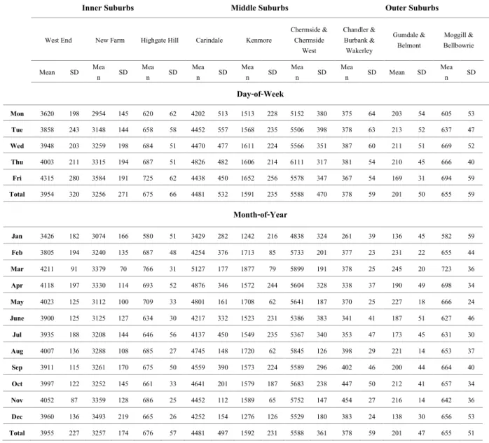
The mean and standard deviation (SD) of daily ridership for all suburbs by day-of-week and month-of-year
1
are presented in the following table (table 2).
2
TABLE 2 Mean ridership and Standard Deviation by Day-of-week and Month-of-year
3
4
Figure 1 represents the difference in mean between original and decomposed ridership by day-of-week and
5
month-of-year of three sample suburbs from three different categories; West End (inner), Carindale (middle), and
6
Gumdale & Belmont (outer). The smoother trend line of weekly and monthly decomposed ridership shows the
7
effectiveness of seasonal decomposition process. This seasonally adjusted data set was used for further analysis.
8
Each suburb’s ridership was converted into its population percentage to scale all suburb’s ridership data.
9
However, one problem persisted. Suburbs including West End and Carindale, which have high job densities, attract
10
a significant numbers of workers each day who are not residents. When they leave the area on their homeward
11
commute, they are counted as a boarding trip originating from that suburb. This produces higher ridership for that
12
particular suburb and does not reveals the real picture of its residents’ ridership. In order to overcome this inflation,
13
each suburb’s job density was added to its population before dividing the average ridership and converting it into a
14
percentage. This method scaled down the suburb’s overstated ridership for unbiased comparison.
15
Inner Suburbs
Middle Suburbs
Outer Suburbs
West End New Farm Highgate Hill Carindale Kenmore Chermside & Chermside West
Chandler & Burbank & Wakerley
Gumdale &
Belmont Bellbowrie Moggill & Mean SD Mean SD Mean SD Mean SD Mean SD Mean SD Mean SD Mean SD Mean SD
Day-of-Week
Mon 3620 198 2954 145 620 62 4202 513 1513 228 5152 380 375 64 203 54 605 53 Tue 3858 243 3148 144 658 58 4452 557 1568 235 5506 398 378 63 213 52 637 47 Wed 3948 203 3259 198 684 51 4470 477 1611 224 5566 351 387 60 211 51 669 52 Thu 4003 211 3315 194 687 51 4826 482 1606 214 6111 317 381 54 210 45 666 40 Fri 4315 280 3584 191 725 62 4438 450 1652 256 5578 347 367 54 169 31 694 59 Total 3954 320 3256 271 675 66 4481 532 1591 235 5588 470 378 59 201 50 655 59Month-of-Year
Jan 3426 182 3074 166 580 51 3429 282 1242 216 4838 324 261 39 136 45 582 59 Feb 3805 194 3240 135 687 48 4254 376 1713 85 5733 201 377 23 231 22 655 44 Mar 4211 91 3379 70 766 31 5127 177 1877 79 5899 191 378 25 245 20 723 36 Apr 4118 197 3330 114 693 52 4876 346 1572 244 5604 328 338 37 190 49 698 34 May 4023 125 3112 100 709 33 4801 161 1708 62 5641 187 370 25 227 18 666 24 June 3900 125 3125 127 634 30 4217 332 1523 231 5386 383 341 41 187 51 627 46 Jul 3935 188 3208 144 646 56 4137 450 1549 235 5367 340 353 47 173 45 631 30 Aug 4007 136 3288 108 685 27 4745 148 1720 62 5845 126 398 29 221 14 653 37 Sep 3911 115 3261 170 675 50 4559 390 1573 224 5589 296 402 46 200 44 664 40 Oct 3997 122 3252 145 661 33 4641 201 1579 187 5683 238 447 50 212 41 657 34 Nov 4052 87 3359 128 686 25 4452 112 1589 65 5752 147 454 27 216 14 642 36 Dec 3960 136 3493 219 665 26 4252 154 1276 126 5529 180 383 24 138 30 656 53 Total 3955 227 3257 174 676 57 4481 497 1592 231 5588 361 378 59 201 47 655 511
2
3
4
5
6
7
8
9
10
FIGURE 1 Suburb’s ridership decomposition by day-of-week (left) and month-of-year (right)
11
Transit Quality of Service Measurement
12
TQoS elements weigh the effectiveness and performance of transit system within a particular area. TCQSM (4) has
13
been used as the central reference to scrutinize spectrum of attributes allied to TQoS. Analysis in any dimension
14
reflected the passengers’ point of view because whatever value public transit has for society stems from its value to
15
its riders. This study evaluates service frequency, service span, and access (via route intensity) as well as travel time
16
ratio factor which is considered under comfort and convenience. This section will explain the calculation method of
17
each variable that has been used in this study during analysis.
18
Bus Service intensity and Service span
19
The measurement of service frequency is a self-explanatory component of TQoS, quantifying the accessibility of the
20
service to its passenger without considerable waiting time. Ubiquitous assumption, allied with some research
21
findings dictates the notion that alteration in service frequency is the key factor that sways ridership from its usual
22
disposition. All other things being equal, if only frequency increased, ridership should increase (4). Therefore, it is
23
important to estimate route service frequency very accurately to understand its effects on regular passengers.
24
Ridership data provided by TransLink only included boardings and therefore, the transit trips originating
25
from a particular suburb. Therefore, the service frequency of particular route was calculated for only one direction,
26
originating from the suburb towards the CBD or a popular destination. Service frequency was calculated for three
27
different periods; Morning Peak (7am – 9 am), Off Peak (9 am – midnight) and frequency throughout the day (7 am
28
– midnight). This enables the effect of different periods’ frequency on ridership to be understood. Calculation of the
29
morning peak frequency as well as the frequency throughout the whole day was restricted from 7 am even though
30
some of services start well before 7 am. The reasoning can be related to the start of morning peak services from 7
31
am prescribed by TransLink, as well as very low ridership. Likewise, services operating after midnight were also not
32
considered.
The number of bus services operating between the start and end of each time period were calculate for all
1
routes servicing each suburb, as along with their service spans. Even though the TCQSM has been used as the
2
reference for calculating the TQoS elements related to this study, service provision was treated differently from the
3
service frequency measure. The method adopted in this research of calculating service intensity has its own merits as
4
it embedded service coverage area with the frequency calculations, amalgamating two TQoS elements as one. This
5
approach provided a holistic view of the condition of transit service in a particular area.
6
The following equation was used to calculate service intensity (bus-km/h-km2):
7
𝑆𝐼 =
(∑𝑛𝑖=1𝑁𝑏𝑢𝑠,𝑖⁄𝑆ℎ𝑟,𝑖) x 𝑅𝑘𝑚,𝑖𝐴𝑠𝑢𝑏𝑢𝑟𝑏
……….. (3)
8
𝑛 = Number of bus routes servicing the suburb
9
𝑁𝑏𝑢𝑠,𝑖= Number of route 𝑖 bus services operating through the suburb
10
𝑆ℎ𝑟,𝑖 = Bus route 𝑖’s number of hours of service through suburb during analysis period
11
𝑅𝑘𝑚,𝑖 = Number of route kilometers of bus route 𝑖 through suburb
12
𝐴𝑠𝑢𝑏𝑢𝑟𝑏 = Area of the suburb in square kilometers.
13
In applying Equation 3, the frequency (bus/hr) of each route servicing the suburb was calculated. For each
14
route, the portion of its length contained within that suburb’s boundary was identified using Google Map embedded
15
in TransLink’s website (32). Areas where people’s dwellings are uncommon (such as park, picnic ground,
16
recreational reserve) were excluded in the suburb area calculation. This service intensity variable (bus-km/h-km2)
17
explains how many km of service is provided per hour in each unit of area through the suburb. This measure
18
amalgamates two TQoS elements, service frequency and route density as one.
19
Typically, service frequency provides information about how frequent bus service is provided from an area
20
but it does not describe how many km of bus route services the area. This information is necessary to understand the
21
ease or difficulty of entree, which riders face when accessing transit. Suburbs with very frequent bus service but
22
confined in very small portion of land area, will have limited transit access for the majority of their population.
23
However, if the service is well spread throughout the suburb, it will attract more patronage. Route intensity
24
describes how frequent bus service is as well as how well spread service is. Based on this analysis, the average
25
service intensityranged from 4.3 to 39.8 bus-km/h-km2.
26
Transit service ought to be available when potential passengers want to travel; otherwise, public transport
27
will not be used by riders even though it is available the rest of the day. Existing service span for each route was
28
collected from TransLink schedules (32). Service span for a particular route was defined as the time difference
29
between the first service entering and the last service leaving the suburb. The direction of travel was outward from
30
the suburb.
31
The following equation was used to calculate the suburb’s weighted service span:
32
33
𝑆𝑝𝑎𝑛 =
∑𝑛𝑖=1𝑆𝑠𝑝𝑎𝑛,𝑖x 𝑁𝑏𝑢𝑠,𝑖 x 𝑅𝑘𝑚,𝑖∑𝑛𝑖=1 𝑁𝑏𝑢𝑠,𝑖 x 𝑅𝑘𝑚,𝑖 ………. (4)
34
𝑆𝑠𝑝𝑎𝑛,𝑖 = service span of bus route 𝑖 through suburb.
35
Travel Time ratio
36
According to TCQSM travel time ratio is measured by dividing the in-vehicle transit travel time with in-vehicle auto
37
travel time (4). This study followed this method. The transportation system of Brisbane is mainly CBD oriented,
38
hence the in-vehicle transit and auto travel times were calculated using the CBD as the destination. Since multiple
39
routes provides service to an area, their mean was obtained when calculating in-vehicle transit travel time. For auto
40
the shortest travel time was used. Times were measured using Google Map 2014 (33), which includes the General
41
Transit Feed Specification (GTFS) in its mapping system.
42
43
Grade Factor
1
Variation in grade was calculated for each suburb following its road network through which people predominantly
2
walk to access transit. ‘Brisbane City Plan 2014 interactive mapping tool’ (34), which provides 1 m contour lines,
3
was used to calculate average grade over 400m walking approaches to bus stops, which were located using ‘Google
4
transit map’ (33). Each suburb’s grade factor was determined using a sample of walking approaches. The average
5
grade factors varied by suburb from 3.5% to 10.8%.
6
Model Estimation and Result
7
Two regression models were estimated to examine the relationship between bus ridership and TQoS in terms of
8
service intensity, service span, travel time ratio and grade. Model 1 separated service intensity into two different
9
periods; peak hour service (7am - 9am) and off-peak hour service (9am - midnight). Model 1 was intended to reflect
10
higher service intensity to serve commuting trips made during the morning peak period, and lower service intensity
11
for the remainder of trips made off-peak.
12
The following Model 1 was calibrated using multiple linear regression:
13
𝑅1= 𝛽𝑆𝐼𝑃,1𝑆𝐼𝑝𝑒𝑎𝑘+ 𝛽𝑆𝐼𝑂,1𝑆𝐼𝑜𝑓𝑓−𝑝𝑒𝑎𝑘+ 𝛽𝑆𝑆,1𝑆𝑆 + 𝛽𝑇𝑇𝑅,1𝑇𝑇𝑅 + 𝛽𝐺𝐹,1𝐺𝐹 + 𝜀1…..……….. (5)
14
𝑅1= Percentage of ridership amongst suburb population
15
𝑆𝐼𝑝𝑒𝑎𝑘 = Peak period service intensity for suburb.
16
𝑆𝐼𝑜𝑓𝑓−𝑝𝑒𝑎𝑘= Off-peak period service intensity for suburb.
17
𝑆𝑆= Service span for suburb
18
𝑇𝑇𝑅= Travel time ratio between in-vehicle transit and automobile time for suburb.
19
𝐺𝐹= Average grade factor of suburb.
20
𝛽𝑆𝐼𝑃,1, 𝛽𝑆𝐼𝑂,1, 𝛽𝑆𝑆,1, 𝛽𝑇𝑇𝑅,1, 𝛽𝐺𝐹,1 = Model constants
21
𝜀1 = Error term.
22
Similarly, Model 2 was calibrated using multiple linear regression:
23
𝑅2= 𝛽𝑆𝐼,2𝑆𝐼𝑑𝑎𝑦+ 𝛽𝑆𝑆,2𝑆𝑆 + 𝛽𝑇𝑇𝑅,2𝑇𝑇𝑅 + 𝛽𝐺𝐹,2𝐺𝐹 + 𝜀2……….. (6)24
Where,25
26
𝑆𝐼𝑑𝑎𝑦 = Whole day service intensity.
27
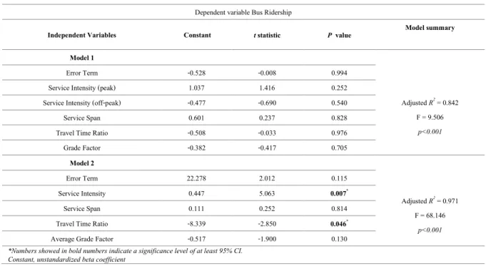
For Model 1, although the adjusted R2 and p value (0.047) were acceptable, all the signs of the coefficients
28
did not blend with the hypothesis of this study. The negative coefficient sign of off-peak hour service intensity was
29
counterintuitive. A possible explanation behind this result is when the peak and off-peak frequency were included
30
together in one model, it resulted in an ambiguity effect. The model estimated the effect of peak frequency on both
31
peak and off-peak ridership (since ridership provided by TransLink was for the entire day). A similar effect occurred
32
for the case of off-peak frequency. Duplicitous effects of peak and off-peak intensity was identified and to balance
33
the equation the model may have produced negative coefficient for off-peak service. Furthermore, none of the
34
variables in Model 1 were significant at all, even though their coefficient signs were as hypothesized (except peak
35
service intensity).
36
In Model 2, a single independent variable was used to reflect service intensity across the whole period
37
between 7am and midnight. A significant improvement was observed in model’s statistical test with higher adjusted
38
R2. The result also indicated no multicollinearity effect among the variables. The high value of adjusted R2 in this
39
model is consistent with other previous research (20) using similar method. Two of explanatory variables (service
40
intensity and travel time ratio, shown in bold) were statistically significant predictors of bus ridership and the
41
constants of all variables indicate that the variables were in the direction expected. Table 3 presents the multiple
42
regression modelling results of the two models for bus ridership from the Brisbane suburbs analysed. The models
43
result includes estimated coefficient (β), t statistics and significance levels (p values) for all explanatory variables.
44
TABLE 3 Summary of Multiple Regression Modelling Results for Two Models
1
2
Figure 2 compares original ridership percentage and percentages estimated using Models 1 and 2. It can be
3
seen that Model 2 produces slightly better estimates of a suburb’s ridership.
4
FIGURE 2 Comparison among original and estimated ridership
5
Meanwhile, both service span and grade factor were found to have non-significant association with bus
6
ridership. In the context of Brisbane city, the result is not surprising. Many parts of Brisbane are hilly. Irrespective,
7
some areas attracts higher ridership compared with areas of flatter terrain. Influences of other variables on ridership,
8
such higher service frequency or lower travel time ratio might be the reason behind this. Even though the grade
9
factor variable was found to be non-significant, the negative coefficientsign showed the expected direction of
10
variable. This result was similar to another previous study for the same region (10). Similarly, the effect of service
11
span was expected to have non-significant result in Brisbane’s context. Extended service spans are usually aspired
12
Dependent variable Bus Ridership
Independent Variables Constant t statistic P value Model summary
Model 1
Adjusted R2= 0.842 F = 9.506
p<0.001
Error Term -0.528 -0.008 0.994
Service Intensity (peak) 1.037 1.416 0.252
Service Intensity (off-peak) -0.477 -0.690 0.540
Service Span 0.601 0.237 0.828
Travel Time Ratio -0.508 -0.033 0.976
Grade Factor -0.382 -0.417 0.705 Model 2 Adjusted R2= 0.971 F = 68.146 p<0.001 Error Term 22.278 2.012 0.115 Service Intensity 0.447 5.063 0.007* Service Span 0.111 0.252 0.814
Travel Time Ratio -8.339 -2.850 0.046*
Average Grade Factor -0.517 -1.900 0.130
*Numbers showed in bold numbers indicate a significance level of at least 95% CI. Constant, unstandardized beta coefficient
for higher activity during late night times. In Brisbane, night time activities tend to diminish substantially after 9p.m.
1
on weeknights. Therefore, providing services for longer hours especially between midnight and dawn does not
2
influence ridership in Brisbane.
3
Finally, the overall outcome of this study exposed new insights into the effect of Transit Quality of Service
4
(TQoS) on a CBD oriented city like Brisbane that confound some popular assumptions about urban transit ridership.
5
The belief that suburbs located in close proximity to a CBD will attract higher ridership is not supported by this
6
study’s preliminary findings. Rather, a suburb can attract higher transit ridership if it is provided with higher transit
7
service facilities regardless of its proximity to a CBD. Comparison between the suburbs of Carindale (middle) and
8
Highgate Hill (inner) illustrate this finding. Highgate Hill is only 2.7 km from the CBD while Carindale is 10.1 km
9
away. Nevertheless, Carindale’s ridership by percentage of population is more than twice that of Highgate Hill.
10
Apart from factors examined here, a further factor that may explain this finding is that active transport use as a
11
principal mode may be higher for Highgate Hill due to its proximity to the CBD, while active transport use is more
12
generally an access mode to transit for Carindale.
13
CONCLUSION AND FUTURE DIRECTION
14
This paper examined the influence of transit facilities on a particular transit performance measure, transit ridership,
15
using a sample of suburbs of Brisbane, Australia as a case study. Data sets for this analysis was attained from
16
TransLink, Brisbane City Council and Google transit map, 2014. All these data provided a robust data frame to
17
study.
18
The statistical analysis observed a strong relationship between explanatory variables (service intensity,
19
service span, travel time ratio and grade factor) and ridership. It revealed that a suburb can attract higher ridership,
20
only if it is facilitated with adequate transit service intensity (bus-km/hr/km2) regardless of its topographical
21
condition and closeness to the CBD. The effect of service intensity showed the highest impact on ridership
22
compared to other variables. The significant negative association of travel time ratio with ridership confirmed that as
23
the transit-auto travel time ratio increased, bus ridership decreased. The outcome of this result did not support some
24
popular views that closeness to a city’s central business district will attract higher ridership. Rather, Brisbane’s bus
25
riders value high service frequency, emulated with higher route coverage. Conversely, the study did not observed
26
any significant influence of grade factor on ridership, opposing views of other studies in the literature that hilly
27
terrain reduces the propensity of walking to access transit and thus its ridership. Similarly, the impact of service span
28
was not found to be influential on bus ridership in the context of Brisbane city.
29
Overall, the findings of this paper are consistent with literature and provide a solid basis for further
30
investigation of transit ridership. However, there are some limitations. The study could not include all the variables
31
related to TQoS mentioned in TCQSM manual. Hence, it will be interesting to explore how the other measures such
32
as passenger load and reliability affect ridership in this city. Likewise, in addition to the natural environment factor
33
of average grade, pedestrian environment such as street connectivity could be considered in future analysis to better
34
understand of walkability effect on travel behaviour. Finally, analysis could include more suburbs to represent
35
Brisbane as a whole.
36
Considering analysis results, this paper provides some valuable insights to transit authorities to diagnose
37
how the overall bus system is performing in different locations and how the existing ridership can be increased
38
considering short-term and long-term approach in some areas. The study concludes that bus service intensity is a key
39
driver of ridership regardless of suburb location. A perfect example is the inner suburb Highgate Hill, which is very
40
close to CBD, resulting minimum travel time ratio. However, due to its lower service frequency and route coverage,
41
sufficient ridership is not generated. On the other hand, middle suburb Chermside / Chermside West generates
42
almost double the ridership, which is attributed to high service frequency and route coverage, despite its higher
43
travel time ratio compared with Highgate Hill. Under a long term approach, bus ridership might be increased by
44
direct routing and expansion of busway and/or bus lane.
45
46
47
ACKNOWLEDGMENT
1
The authors thank Briohny Rootman and Tristan Miles (Senior Network Analyst) TransLink Division, Department of
2
Transport and Main Roads (TMR), Queensland, who provided invaluable ridership data and support for this study.
3
4
REFERENCES
5
1.
Zarei, H. Relationship Between Non-Auto Travel and Characteristics of the Built Environment and Trip6
Makers: Empirical Analysis and Case Study. MS thesis. 2007. University of Toronto, Ontario, Canada.
7
2. Cervero, R., and K. Kockelman. Travel Demand and the 3Ds: Density, Diversity, and Design. Transportation
8
Research, Vol. 2, No. 3, 1997, pp.199–219.
9
3. Hendricks, S. J. Impacts of Transit Oriented Development on Public Transportation Ridership. Final Report by
10
National Center for Transit Research Center for Urban Transportation Research. University of South Florida
11
Report Number BD549-05, 2005.
12
4. TRB. Transit Capacity and Quality of Service Manual (TCQSM), 3rd Edition, 2013. Available from:
13
http://www.trb.org/. Accessed January. 27, 2014.
14
5. Muley,D., J. M. Bunker, and L. Ferreira. Evaluating transit Quality of Service for Transit Oriented
15
Development (TOD). Evaluating transit Quality of Service for Transit Oriented Development (TOD). In 30th
16
Australasian Transport Research Forum (ATRF), September. 25-27, 2007, Melbourne, Australia.
17
6. Brisbane Metropolitan Transport Management Centre, Busway Operations Centre.
18
http://www.bmtmc.com.au/index.php/entry/4. Accessed May 12. 2013.
19
7. National Research Council. TCRP Report 145: Reinventing the Urban Interstate: A New Paradigm for
20
Multimodal Corridors. Washington, DC: The National Academies Press, 2011.
21
8. Australian Bureau of statistics (ABS). http://www.abs.gov.au/. 2011. Accessed January 10, 2014.
22
9. Sarkar, S. Qualitative evaluation of comfort needs in urban walkways in major activity centers. Transportation
23
Quarterly, Vol. 57, No. 4, 2003, pp. 39-59.
24
10. Burke, M., N. Sipe, R. Evans, and D. Mellifont. Climate, geography and the propensity to walk: environmental
25
factors and walking trip rates in Brisbane. In 29th Australasian Transport Research Forum (ATRF), Australia.
26
11. Cervero, R., S. Murphy, C. Ferrell, N. Goguts, Y. Tsai, Parsons Brinckerhoff Quade and Douglas, Inc., Bay
27
Area Economics, Urban Land Institute. 2004. Transit Oriented Development in America: Experiences,
28
Challenges, and Prospects, Transit Cooperative Research Program, Transportation Research Board, National
29
Research Council, Washington, D.C., p. 7.
30
12. Ewing, R., and R. Cervero. Travel and the built environment: a synthesis. In Transportation Research Record:
31
Journal of the Transportation Research Board, No. 1780, Transportation Research Board of the National
32
Academies, Washington, D.C., 2001, pp. 87–122.
33
13. Frank, L., and G. Pivo. Impacts of mixed use density on utilization of three modes of travel: single-occupant
34
vehicle, transit, and walking. In Transportation Research Record: Journal of the Transportation Research
35
Board, No. 1466, Transportation Research Board of the National Academies, Washington, D.C., 1994, pp. 44–
36
52.
37
14. Dannenburg AL, RJ. Jackson, H. Frumkin, RA.Schieber, M. Pratt , C. Kochtitzky , HH. Tilson. The impact of
38
community design and land-use choices on public health: a scientific research agenda. Am J Public Health. Vol.
39
93:1500–8, 2003.
40
15. Frank, L. D., TL. Schmid, JF. Sallis, J. Chapman, and BE. Saelens. Linking objectively measured physical
41
activity with objectively measured urban form: findings from SMARTRAQ. Am J Prev Med. Vol. 28(2 Suppl
42
2):117-25, 2005.
43
16. Lavizzo-Mourey, R, and JM. McGinnis. Making the case for active living communities. Am J Public Health.
44
Vol. 93:1386–8, 2003.
45
17. Kain, J.F. and Z. Liu. Econometric Analysis of Determinants of Transit Ridership: 1960-1990. Prepared for the
46
Volpe National Transport Systems Center, U.S. Department of Transportation, 1996.
18. Gomez-Ibanez, J. A.Big-city transit, ridership, deficits, and politics. Journal of the American Planning
1
Association. Vol. 62, No.1, 1996, pp. 30-50.
2
19. Litman, T. Valuing Transit Service Quality Improvements. Journal of Public Transportation. Vol.11, No.2,
3
2008, pp. 43-63.
4
20. Kohn, H. M. Factors Affecting Urban Transit Ridership. In Bridging the Gaps Conference, Canadian
5
Transportation Research Forum, June 6, 2000, Canada.
6
21. Daskalakis, N. G., and A. Statopoulos. Users' Perceptive Evaluation of Bus Arrival Time Deviations in
7
Stochastic Networks. Journal of Public Transportation. Vol. 11, No. 4, 2008, pp. 25-38.
8
22. Cervero, R. Transit Pricing Research: A Review and Synthesis.Transportation. Vol. 17, 1990, pp. 117-139.
9
23. Syed, S. J., and A.M. Khan. Factor Analysis for the Study of Determinants of Public Transit Ridership.Journal
10
of Public Transportation. Vol. 3, No. 3, 2000, pp. 1-17.
11
24. Caulfield, B., and M. O'Mahony. A Stated Preference of Analysis of Real-Time Public Transit Stop
12
Information. Journal of Public Transportation. Vol. 12, No. 3, 2009, pp.1-20.
13
25. Abdel-Aty, M. A., and P. P. Jovanis. The Effect of ITS on Transit Ridership. ITS Quarterly. 1995, pp. 21-25.
14
26. Thompson, G., J. Brown, and T. Bhattacharya. What Really Matters for Increasing Transit Ridership:
15
Understanding the Determinants of Transit Ridership Demand in Broward County, Florida. Urban Studies. Vol.
16
49, No. 15, 2012, pp. 3327-3345.
17
27. Liu, R., S. Polzin, and R. Pendyala. Simulation of the Effects of Intermodal Transfer Penalties on Transit Use.
18
Transportation Research Record, No. 1623, Transportation Research Board, National Research Council,
19
Washington, D.C., 1998, pp. 88-95.
20
28. Krizek, K. J., and A. M. El-Geneidy. Segmenting Preferences and Habits of Transit Users and Non-Users.
21
Journal of Public Transportation. Vol. 10, No. 3, 2007, pp. 71-94.
22
29. Holtzclaw, J. Using Residential Patterns and Transit to Decrease Auto Dependence and Costs. New York:
23
Natural Resources Defence Council. 1994.
24
30. Parsons Brinkerhoff, Quade and Douglas Inc, Cambridge Systematics Inc, and Calthorpe Associates. 1000
25
Friends of Oregon,Making Land Use Transportation Air Quality Connection: the pedestrian environment.
26
Portland, Oregon, US, 1993. http://ntl.bts.gov/DOCS/tped.html. Accessed July 10, 2014.
27
31. Hinchliffe, S. South East Queensland Regional Plan 2009–2031. Department of Infrastructure and Planning.
28
2009.
29
32. TransLink. The Department of Transport and Main Roads (TMR), Queensland Government.
30
http://translink.com.au/. Accessed May 12. 2013.
31
33. Google transit map, Brisbane, 2014.
https://www.google.com.au/maps/place/Brisbane+QLD/@-32
27.3955026,152.9083549,11z/data=!4m2!3m1!1s0x6b91579aac93d233:0x402a35af3deaf40?hl=en. Accessed
33
July 20, 2014.
34
34. Brisbane City Plan 2014 interactive mapping,Dedicated to a better Brisbane. Brisbane City Council (BCC).
35
http://cityplan2014maps.brisbane.qld.gov.au/CityPlan/. Accessed May 15, 2014.
36
35. Kashfi, S. A., B. Lee, and J. Bunker. Impact of rain on Daily Bus ridership: A Brisbane Case Study.
37
Australasian Transport Research Forum 2013 Proceeding. October, 2-4, 2013, Brisbane, Australia.