econstor
www.econstor.eu
Der Open-Access-Publikationsserver der ZBW – Leibniz-Informationszentrum Wirtschaft The Open Access Publication Server of the ZBW – Leibniz Information Centre for EconomicsNutzungsbedingungen:
Die ZBW räumt Ihnen als Nutzerin/Nutzer das unentgeltliche, räumlich unbeschränkte und zeitlich auf die Dauer des Schutzrechts beschränkte einfache Recht ein, das ausgewählte Werk im Rahmen der unter
→ http://www.econstor.eu/dspace/Nutzungsbedingungen nachzulesenden vollständigen Nutzungsbedingungen zu vervielfältigen, mit denen die Nutzerin/der Nutzer sich durch die erste Nutzung einverstanden erklärt.
Terms of use:
The ZBW grants you, the user, the non-exclusive right to use the selected work free of charge, territorially unrestricted and within the time limit of the term of the property rights according to the terms specified at
→ http://www.econstor.eu/dspace/Nutzungsbedingungen By the first use of the selected work the user agrees and declares to comply with these terms of use.
zbw
Leibniz-Informationszentrum Wirtschaft Leibniz Information Centre for EconomicsPolasky, Stephen; de Zeeuw, Aart; Wagener, Florian
Working Paper
Optimal management with potential regime shifts
CESifo working paper: Resource and Environment Economics, No. 3237
Provided in Cooperation with:
Ifo Institute – Leibniz Institute for Economic Research at the University of Munich
Suggested Citation: Polasky, Stephen; de Zeeuw, Aart; Wagener, Florian (2010) : Optimal management with potential regime shifts, CESifo working paper: Resource and Environment Economics, No. 3237
This Version is available at: http://hdl.handle.net/10419/46395
Optimal Management with Potential
Regime Shifts
Stephen Polasky
Aart de Zeeuw
Florian Wagener
CES
IFO
W
ORKING
P
APER
N
O
.
3237
C
ATEGORY9:
R
ESOURCE ANDE
NVIRONMENTE
CONOMICSN
OVEMBER2010
PRESENTED AT CESIFO AREA CONFERENCE ON ENERGY &CLIMATE ECONOMICS,OCTOBER 2010
An electronic version of the paper may be downloaded
• from the SSRN website: www.SSRN.com
• from the RePEc website: www.RePEc.org
CESifo Working Paper No. 3237
Optimal Management with Potential
Regime Shifts
Abstract
We analyze how the threat of a potential future regime shift affects optimal management. We use a simple general growth model to analyze four cases that involve combinations of stock collapse versus changes in system dynamics, and exogenous versus endogenous probabilities of regime shift. Prior work in economics has focused on stock collapse with endogenous probabilities and reaches ambiguous conclusions on whether the potential for regime shift will increase or decrease intensity of resource use and level of resource stock. We show that all other cases yield unambiguous results. In particular, with endogenous probability of regime shift that affects system dynamics the potential for regime shift causes optimal management to become precautionary in the sense of maintaining higher resource stock levels.
JEL-Code: C61, Q20, O40, E61.
Keywords: optimal management, growth, renewable resources, regime shifts.
Stephen Polasky
Department of Applied Economics University of Minnesota
1994 Buford Ave. USA – St. Paul, MN 55108
[email protected] Aart de Zeeuw
Tilburg University / The Netherlands [email protected]
Florian Wagener
University of Amsterdam / The Netherlands [email protected]
3 1. Introduction
Complex dynamic systems can undergo changes in interactions between constituent components that cause a shift to different system dynamics. In ecological systems such “regime shifts” can cause changes in nutrient cycling and population dynamics of various species with consequences for the value of ecosystem services derived from the system. For example, lakes may shift between oligotrophic and eutrophic conditions with impacts on water quality, fish populations, recreation, and aesthetics (Scheffer 1997, Carpenter et al. 1999, Carpenter 2003). Terrestrial systems can shift between grasslands and woodlands with impacts on the value of grazing and other ecosystem services (Perrings and Walker 1997, Janssen et al. 2004). Coral reef systems can shift from coral dominated to algal dominated with impacts on water quality, fish populations, recreation and aesthetics (Hughes et al. 2003). At a larger scale, the global climate system may have regime shifts with potentially major consequences in several dimensions (e.g., sea level rise, agricultural production, water scarcity). Economic systems can also undergo regime shifts. Examples include sudden shifts in consumer choices (“fads”) and cultural change (e.g., Bikhchandani et al. 1992, and popularized by Gladwell 2000), shifts in financial markets due to changes in investor sentiment and herd behavior (e.g., Scharfstein and Stein 1990, Banerjee 1992, Brock and Hommes 1998) or due to changes in investor information and hedging (Genotte and Leland 1990, Brock et al. 2009), and shifts in the macro-economy (e.g., Azariadis 1981, Cass and Shell 1983, Hamilton 1989, Guo et al. 2005). Once a threshold between regimes has been crossed it may be difficult to reverse the process to shift back to the original regime (“system hysteresis”, Scheffer et al. 2001).
In this paper we analyze optimal management of a dynamic system with the potential for a regime shift. To fix ideas, we focus our discussion on the case of harvesting a
4
renewable resource (e.g., a fishery) in which the growth function of the stock is dependent on the regime and where the stock level of the resource can influence the probability of a regime shift. For example, high levels of harvest can reduce fish populations that graze on plankton and increase the probability that a bleaching event or other disturbance will shift a coral reef system from coral dominated to algal dominated (Hughes et al. 2003). The shift into a new regime reduces fishery productivity and may also reduce other ecosystem services (recreation, storm protection, etc). The model we analyze, however, is more general than harvesting a renewable resource and could be used to analyze any circumstance in which management actions affect probabilities of regime shift, such as greenhouse gas emissions and climate regime shifts, or financial regulations and the potential for sudden shifts in investor sentiment. Prior research in economics on optimal management with potential regime shift has focused on the case of catastrophic stock collapse. In environmental economics, this line of research began with Cropper (1976) who analyzed a model in which utility falls to zero once a threshold is crossed.1 In Cropper’s model, the location of the threshold is unknown. The
probability of crossing the threshold increases in the level of pollution (or resource depletion). William Reed showed how to transform the optimal management problem with a probability of crossing a threshold, which is a stochastic dynamic problem, into a deterministic problem that could be solved analytically using the Pontryagin maximum principle (Reed 1987, 1988; and see Reed and Echavarria Heras 1992 for a useful summary). In Reed’s approach, the potential for collapse has an ambiguous effect on management prior to the collapse. The potential for collapse tends to increase exploitation because collapse reduces the future value of stocks so there is less incentive to maintain stocks. This effect works identically to an increase in the discount rate and occurs for the same reason that an increase in mortality risk increases an individual’s discount rate. Working in the opposite direction, however, is the
1
Earlier, Kamien and Schwarz (1971) developed a model of machinery failure that is formally similar to models of environmental collapse.
5
fact that decreased exploitation results in higher stocks and lowers the probability of collapse. We refer to actions that lessen exploitation to reduce probabilities of bad future outcome as “precaution”. Combining these two effects yields an ambiguous overall result. Reed applied his approach to analyze optimal management of forests subject to fire (Reed 1984, 1987, 1989), fisheries subject to collapse (Reed 1988) and environmental pollution (Clarke and Reed 1994). Threshold models have also been applied by other researchers to climate change (e.g., Tsur and Zemel 1996, Gjerde et al. 1999, Keller et al. 2004), environmental pollution (Tsur and Zemel 1998), groundwater aquifers (Tsur and Zemel 1995), and nuclear power (Aronsson et al. 1998). Mäler et al. (2007) apply a similar model to generate a shadow price for resilience, where resilience influences the probability of regime shift. A slightly different modeling approach to thresholds was taken by Nævdal (2001, 2003, 2006) who does not include the potential for shocks so that the probability of regime shift is positive only in time periods when stocks are being depleted. Tsur and Zemel (2006, 2008) study the regulation of stock externalities that arise in cases of non-cooperative behavior. In all of these models, a regime shift triggers a discontinuous decline in a state variable and/or value function.
A different approach, and one more in line with the ecological literature, is to model a regime shift as a change in system dynamics rather than as a sudden collapse in the stock. Peterson, Carpenter and Brock (2003) consider a model with two regimes (oligotrophic and eutrophic lake system), with state equations that differ by an additive term. They show that optimal management will typically involve periodic collapse (switch from oligotrophic to eutrophic) and recovery (switch from eutrophic to oligotrophic). Brozovic and Schlenker (2008) use a similar model of regime shift to analyze the relationship between precaution and variance of uncertainty and find that the relationship is not monotonic. An increase in the variance of the stochastic component of the natural system that determines whether the threshold is crossed initially increases precaution. However, if the variance gets very large,
6
not much can be done to prevent crossing the threshold and precaution becomes too costly compared to the small reduction in the probability that the threshold is crossed. Brock and Starrett (2003) and Mäler et al. (2003) analyze a model with a convex-concave regeneration function that captures the potential for regime shifts. These models, however, are deterministic and focus on characterizing different optimal paths under various parameter conditions.
In this paper we develop a general growth model with stochastic regime shift that can capture changes to stock levels and/or system dynamics when a regime shift occurs. We consider cases in which the probability of a regime shift is not affected by any management action (exogenous regime shift), and cases in which the probability of a regime shift is a function of management action (endogenous regime shift). The model in this paper contains one important simplification. We assume that the objective function is linear in the control variable, which generates extreme controls and allows for a relatively simple analytical solution.
In the case with an exogenous regime shift that results in a change in system dynamics but not an immediate change in stock level, we show that the threat of regime shift does not affect optimal management prior to any potential regime shift. With an endogenous regime shift that changes system dynamics, optimal management becomes precautionary in the sense that the potential for regime shift will cause managers to choose less intensive harvest (emissions) and maintain higher resource stocks (environmental quality). These results contrast with the prior literature that focused on stock collapse where a potential regime shift causes more intensive exploitation (in the case with exogenous regime shift) or ambiguous results (in the case with endogenous regime shift).
In the next section we set up the optimal management model with potential regime shifts and derive results. The results are discussed in section 3. We compare our results with
7
prior literature and explain major differences. We summarize our findings and include a brief discussion of important extensions and open questions in section 4.
2. Model
We use a simple dynamic model with a linear objective function (constant price and constant marginal cost of harvest) to demonstrate results about optimal management with the potential for a regime shift. The linear objective function in the control variable simplifies the analytics. Other than this, however, the model is quite general. For concreteness and to make comparisons with prior literature easier, we interpret the model as a renewable resource model. The renewable resource can be thought of as a traditional renewable resource like a fishery or as an environmental resource like the global atmosphere. Additional harvest of fish, or increased emission of greenhouse gases, generates extra current flow benefits but leads to depletion of the resource base, which pushes the system in an undesirable direction and makes it more likely that some shock or disturbance will cause regime shift.
The objective is to maximize the present value of revenue from harvest, subject to stock dynamics , all for 0 ) ( , 0 ) ( , ) 0 ( ), ( )) ( ( ) ( s.t. ) ( 0 0 t t h t s s s t h t s G t s dt t ph e Max rt ≥ ≥ = − =
∫
∞ − ɺ (1)where p > 0 denotes the constant net price, h(t) is the harvest level at time t, r > 0 is the discount rate, s(t) is the resource stock at time t, and G(s(t)) is the natural growth function of the resource, which depends on the resource stock. We assume that the growth function is concave in stock and that G(0) = 0.
At some future time τ (possibly infinite) there is a regime shift. Before time τ the growth function is given by G1(s), with G1(s) > 0 for 0 < s < K1 and G1(s) < 0 for s > K1. In
8
given by G2(s), with G2(s) > 0 for 0 < s < K2 and G2(s) < 0 for s > K2. We assume that G1(s)
> G2(s) and G1'(s)>G2'(s), for all s > 0, and K2 < K1. Here Ki, i = 1, 2, can be thought of as carrying capacity, i.e. the steady-state value in the system with no harvest. The size of the stock at time τ is unchanged by the regime shift. Stock dynamics are characterized by
≥ − < ≤ − = − =
τ
τ
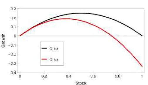
t t h t s G t t h t s G t h t s G t s for ), ( )) ( ( 0 for ), ( )) ( ( ) ( )) ( ( ) ( 2 1 ɺ . (2)A simple illustration of the effect of the regime shift for the case of logistic growth, Gi(s) =
gs(1 - s/Ki), i = 1, 2, with g = 1, K1 = 1 and K2 = 0.75, is shown in Figure 1.
Figure 1: Illustration of a reduced growth function after a regime shift.
In the case where regime shift causes stock collapse, we have s(t) = 0 and G2(0) = 0
for all t ≥τ.
We think of the regime shift as a future event where the time until this event occurs is a stochastic variable. The standard way of modeling this is by means of a hazard rate λ. If the hazard rate is constant, the time until the event occurs is drawn from an exponential probability distribution λe-λx where a high λ means a high probability that the event will happen soon. Alternatively, 1/λ can be seen as an indicator of the resilience of the system,
9
i.e., its ability to resist shocks and maintain current productivity even with disturbance (note that 1/λ is the mean of the exponential probability distribution). We will, however, also consider hazard rates that depend on the stock, λ(s), in order to capture the possibility that harvesting behavior that changes stock levels will affect the probability of a regime shift.
In the case where regime shift causes a shift in system dynamics, we have a standard renewable resource model with growth function G2(s) after the shift has occurred. The
optimal harvesting policy in this second regime is well-known and can be derived with a “most rapid approach path” technique (Spence and Starrett 1975). However, we will show the result with dynamic programming as that technique can also be used when analyzing the first regime before the shift has occurred. Except for discounting, the problem is stationary and the Hamilton-Jacobi-Bellman equation for the current value function V2 is given by
)} ) ( )( ( ' ) ( { max 0 ph rV2 s V2 s G2 s h h − + − = . (3)
Because this equation is linear in h, the optimal harvest has three basic options with h = 0 when p<V2'(s), h infinite when p>V2'(s), and h indeterminate when p=V2'(s). We have to find the value function V2 that satisfies the Hamilton-Jacobi-Bellman equation. We will
work in steps: first we fix a maximal harvest level hm large enough so that the stock always
decreases for h = hm, and determine the solution V2 of this problem, and then we take the
limit hm →∞ in V2. Given the structure of the optimal harvest, the idea is to split the state
space of s between 0 and the carrying capacity K2 in an area where h = 0, so that the state
increases, and an area where h = hm, so that the state decreases, separated by a singular state
s2. We will construct the value function V2 from the resulting differential equations and we
will show that the conditions of the Hamilton-Jacobi-Bellman equation (3) are fulfilled, so that this is indeed the structure of the optimal solution. This procedure leads to the following set of differential equations:
10 > − + − = < + − = (4b) . for ), ) ( )( ( ' ) ( 0 (4a) , for ), ( ) ( ' ) ( 0 2 2 2 2 2 2 2 2 s s h s G s V s rV ph s s s G s V s rV m m
Differentiation and algebraic manipulation of equations (4a) and (4b) yields
> − − − = < − = . for , ) ) ( ( ) ( )) ( ' ( ) ( '' , for , )) ( ( ) ( )) ( ' ( ) ( '' 2 2 2 2 2 2 2 2 2 2 2 2 s s h s G ph s rV s G r s V s s s G s rV s G r s V m m (5)
Let the state s2 be determined by
r s
G2'( 2)= . (6)
Assuming that G2'(0)>r, the state s2 is situated between 0 and the carrying capacity K2. It is
clear from equation (1) that 0 < V2(s) < phm/r. Therefore, it follows from equation (5) and
the concavity of G2(s) that V2 ''(s) is negative for s < s2 and also negative for s > s2, so that
V2’ is decreasing. In the limit as s approaches s2 from below in (4a) and s approaches s2 from
above in (4b), these equations can be interpreted as two equations in the two unknowns V2(s2)
and V2’(s2), if the function V2 is continuously differentiable. This leads to
. ) ( ) ( , ) ( ' 2 2 2 2 2 2 r s pG s V p s V = = (7)
Because V2’ is decreasing, if follows that V2'(s)> p for s < s2 and V2'(s)< p for s > s2, so that h = 0 and h = hm are indeed the optimal harvest levels for s < s2 and s > s2, respectively.
The state s2 is a steady state with optimal harvest h = G2(s2) and a value given by the second
equation in (7). All the conditions of the Hamilton-Jacobi-Bellman equation (3) are satisfied. The structure of the optimal solution in the second regime is clear now. It consists of the steady-state path s = s2, where s2 is determined by equation (6), preceded by a path with h =
0 if we start at a stock s below s2, or by a path with h = hm if we start at a stock s above s2.
Equation (6) is the standard “golden rule” of growth. The value function V2 can be
11 > − + < = − − − 2 ) ( 2 2 ) ( 2 2 2 ) ( 2 for , ) 1 ( ) ( for , ) ( ) ( 0 s s r ph e r s pG e s s r s pG e s V m s rt s rt s rt m m , (8)
where t0(s) and tm(s) can be interpreted as the times needed to reach s2 from s with h = 0 and
h = hm, respectively. These functions satisfy t0'(s)=−1/G2(s) and tm'( )s =1 / (hm −G s2( )). We now take the limit of the value function V2 for s > s2, given by equation (8), for hm→∞.
It is clear that tm(s) → 0. Furthermore, since limx→0 (1-e-x)/x = 1, we have that
) ( ) ( lim ) ( ) ( 1 lim 2 2 ) ( 2 2 s s p dx p dx x G h h p ph s t s rt e s s s s m m h m m m s rt h m m m − = = − = −
∫
∫
∞ → − ∞ → . (9)In the limit for hm→∞, the, the value function V2(s) for s > s2 takes the form
2 2 2 2 2 ,for ) ( ) ( ) ( s s r s pG s s p s V = − + > . (10)
The interpretation of equation (10) is that the amount (s - s2) is harvested instantaneously and
sold at price p and from that point on there is a steady-state harvest equal to natural growth, G2(s2). Since the conditions in the first regime are better than the conditions in the second
regime, it is to be expected that expression (10) for the value function V2 is the relevant one
when the regime shift occurs.
Deriving the value function in the case where a regime shift causes a stock collapse is trivial since s(t) = 0, so that h(t) = 0 for all t ≥τ. Therefore, we have that V2(s) = 0 for all s.
Next we consider the first regime, before the possible event. Harvest levels h must maximize the expected present value of net revenue
2 0 1 0 { ( ) ( ( ))} s.t. ( ) ( ( )) ( ), (0) , ( ) 0, ( ) 0 for all , rt r MaxE e ph t dt e V s s t G s t h t s s s t h t t τ τ
τ
− + − = − = ≥ ≥∫
ɺ (11)where τ is a stochastic variable. For a constant hazard rate λ, with an exponential probability distribution for the point in time τ, a Pontryagin approach for deriving the optimal solution is
12
convenient (see appendix 1). However, we want to consider the possibility that the hazard rate λ is not constant and that it depends on the stock s. This can be solved with a Pontryagin approach as well (see appendix 1) but this is much more tedious and we prefer to develop the Hamilton-Jacobi-Bellman equation for the value function in the first regime, directly using the hazard rate.
Starting at time t with stock s we can approximate the probability of a regime shift in a small time period ∆t by λ(s(t))∆t, which is in fact the basic definition of the hazard rate λ. The value function, W1(s,t), is the maximal expected value of the objective function at time t
for stock s and can therefore be written as
1 ( ) 1 2 ( , ) max{ ( ) (1 ( ) ) ( , ) ( ) ( )} t t rx h t r t t W s t e ph x dx s t W s s t t s te V s s
λ
λ
+∆ − − +∆ = + − ∆ + ∆ + ∆ + ∆ + ∆∫
. (12)We use the symbol W because we want to use the symbol V when we eliminate the factor e-rt from the resulting Hamilton-Jacobi-Bellman equation below. By approximating the integral and moving the left-hand side of equation (12) to the right-hand side and dividing by ∆t, we get ( ) 2 1 1 1 0 max{ ( ) ( ) ( ) ( , ) ( , ) ( , ) } rt r t t h e ph s e V s s s W s s t t W s s t t W s t t
λ
λ
− − +∆ = + + ∆ − + ∆ + ∆ + ∆ + ∆ − + ∆ . (13)Taking the limit of equation (13) for ∆t→0 yields
2 1 1 1 1
0 max{ rt rt ( ) ( ) ( ) ( , ) s( , )( ( ) ) t( , )}
h e ph e
λ
s V sλ
s W s t W s t G s h W s t− −
= + − + − + . (14)
Except for discounting, the problem is stationary again. By defining V1(s) = ertW1(s,t), the
Hamilton-Jacobi-Bellman equation for the first regime becomes )} ) ( )( ( ' ) ( )) ( ) ( )( ( { max 0 ph s V2 s V1 s rV1 s V1 s G1 s h h + − − + − = λ . (15)
The structure of equation (15) is the same as the structure of equation (3). The optimal harvest in the first regime has three basic options as well, with h = 0 when p<V1'(s), h
13
infinite when p>V1'(s), and h indeterminate when p=V1'(s). Again, we first impose the restriction 0
≤
h ≤ hm. As before we search for a positive state s1, below the carrying capacityK1, with h = 0 for s < s1 and h = hm for s > s1, so that all the conditions of the
Hamilton-Jacobi-Bellman equation (15) are satisfied. If h = 0 and h = hm are the optimal harvest levels,
equation (15) yields > − + + − + = < + + − = ) 16b ( for ), ) ( )( ( ' ) ( )) ( ( ) ( ) ( 0 ) 16a ( for ), ( ) ( ' ) ( )) ( ( ) ( ) ( 0 1 1 1 1 2 1 1 1 1 2 s s h s G s V s V s r s V s ph s s s G s V s V s r s V s m m
λ
λ
λ
λ
In the limit as s approaches s1 from below in (16a) and s approaches s1 from above in (16b),
these equations yield two equations in the two unknowns V1(s1) and V1’(s1), if the function V1
is continuously differentiable. This leads to
) ( ) ( ) ( ) ( ) ( , ) ( ' 1 1 2 1 1 1 1 1 1 1 s r s V s s pG s V p s V λλ + + = = . (17)
Differentiation of equations (16a) and (16b) yields
> = − < = , for ), ( ) ( '' ) ) ( ( , for ), ( ) ( '' ) ( 1 1 1 1 1 1 s s s f s V h s G s s s f s V s G m (18) where )) ( ) ( )( ( ' ) ( ' ) ( ) ( ' )) ( ' ) ( ( ) (s r s G1 s V1 s s V2 s s V1 s V2 s f = +
λ
− −λ
+λ
− . (19)In order for h = 0 and h = hm to be the optimal harvest levels, we need that V1'(s)> p for s < s1 and V1'(s)< p for s > s1. As a consequence, with equation (17), we need the left limit and the right limit of V1 ''(s) at s = s1 to be less than or equal to 0. It follows from equation (18)
that this is equivalent to f(s) ≤ 0 for s < s1 and f(s) ≥ 0 for s > s1, so that the state s1 must
satisfy f(s1) = 0 or, using equations (19) and (17),
− + + − + = ( ) ( ) ) ( ) ( ' ) ( ' 1 ) ( ) ( ' 1 1 2 1 1 1 1 2 1 1 1 V s p r s G s r s p s V s r s G λ λ λ . (20)
14
The difficulty here is that we cannot generally show that f(s) < 0 for s < s1 and f(s) > 0 for s
> s1, as we had in the analysis of the second regime. It is reasonable to assume that
0 ) ( ' s <
λ , because the resilience 1/λ(s) should increase if the stock s increases, and that 0
) ( ' K1 =
λ
. Furthermore, we assume that G1'(0)> +rλ
(0). This guarantees that f(0) < 0 and f(K1) > 0, so that somewhere on the interval (0, K1) the function f is zero and switchessign from negative to positive. Note, however, that the function f may have multiple zeros. If f switches from positive to negative, the solution of equation (20) separates areas where h = hm to the left and h = 0 to the right. These points are not stable. We cannot rule out the
existence of more than one stable steady state, however, so that the optimal solution may depend on the initial state. If there is an interval of singular states, instead of an isolated one, we need to have V1'(s)= p on that interval. It follows from equation (15) that equation (17) and thus equation (20) have to hold on the whole interval. This is generally not possible. In what follows, we will focus on a steady state s1, satisfying equation (20) with f(s) < 0 for s <
s1 and f(s) > 0 for s > s1 in some neighborhood of s1. The function V1 satisfying the
differential equation (16), with initial condition (17), solves the Hamilton-Jacobi-Bellman equation (15) in this neighborhood. It follows that the optimal solution here consists of a steady-state path s = s1, with h = G1(s), either preceded by a path with h = 0 if we start at a
stock s below s1, or by a path with h = hm if we start at a stock s above s1. We note that if f
has multiple zeros, say s1 (1)
and s1 (2)
, then there may be an intermediate point s1 (1)
<s 1 (1)
<s1 (2)
such that V1 is continuous but not necessarily differentiable at s 1 (1)
. We show in appendix 2 that even in this case, the function V1 furnishes a solution of the optimization problem.
15
Equation (20) is the “golden rule” of growth when there is the possibility of a regime shift. Our results will follow directly from this golden rule so that we do not give an explicit expression for the value function V1 where hm→∞.2
3. Results
We can use the results of the analysis summarized in equation (20) to provide a characterization of the effects of regime shift on optimal management. We distinguish four cases: a) exogenous regime shift with stock collapse, b) endogenous regime shift with stock collapse, c) exogenous regime shift with changed system dynamics, and d) endogenous regime shift with changed system dynamics.
Case 1: Exogenous regime shift with stock collapse
With a constant hazard rate λ and a stock collapse, we have that λ'(s)=0 and V2 = 0 so that
the condition for the steady-state stock prior to a regime shift (as shown in equation (20)) becomes . ) ( ' 1 1 s =r+
λ
G (21)This result shows that potential future regime shift increases the discount rate leading to a lower steady-state stock than without the possibility of collapse.
Case 2: Endogenous regime shift with stock collapse
If the hazard rate λ depends on the stock s, the condition for the steady-state stock prior to a regime shift with potential total stock collapse V2 = 0 becomes
. ) ( ) ( ) ( ' ) ( ) ( ' 1 1 1 1 1 1 1 s r s G s s r s G
λ
λ
λ
+ + + = (22)16
In this case we have two effects and the net effect is ambiguous (note that λ'(s)<0). The effect shown in Case 1 above (the addition of the term λ(s)) will tend to increase the intensity of harvest and decrease the steady-state stock. However, the desire to avoid a regime shift will tend to decrease the intensity of harvest and increase the steady-state stock
because the final term
) ( ) ( ) ( ' 1 1 1 1 s r s G s λ λ
+ in equation (22) is negative. This can be seen as a form of endogenous discounting. The overall effect is ambiguous. The effect of the potential regime shift on steady-state stock will depend on which effect dominates. The previous literature has focused on this case (e.g., Reed 1988, Clarke and Reed 1994, Tsur and Zemel 1996).
Case 3: Exogenous regime shift with changed system dynamics
If the hazard rate λ is constant and the regime shift causes a shift in system dynamics we have that λ'(s)=0 and V2'(s1)= p so that the condition for the steady-state stock prior to a regime shift becomes . ) ( ' 1 1 s r G = (23)
The steady-state stock in this case is the same as without the possibility of a regime shift. An exogenous probability of regime shift that causes a change in system dynamics, but not an immediate change in stock levels, will not change optimal management. Remember that s1 is
larger than s2 (determined by equation (6)) because of the conditions on the growth functions
G1 and G2 in section 2. If the regime shift occurs, management will adjust to the new
situation, with a lower steady-state value. However, prior to regime shift it is optimal to manage according to the current (not future) conditions.
17
If the hazard rate λ depends on the stock s and a regime shift causes a shift in system dynamics, the condition for the steady-state stock prior to a regime shift becomes
− + + = ( ) ( ) ) ( ) ( ' ) ( ' 1 1 2 1 1 1 1 1 V s p r s G s r s r s G
λ
λ
(24)which can be rewritten as
. ) ( ) ( ) ( ) ( ' ) ( ' 1 1 2 1 1 1 1 1 − + + = V s r s pG p r s r s r s G λ λ (25)
The term between brackets is positive which can be seen as follows. With initial state s1, the
objective in (11) is maximized by h = G1(s1). It follows that
1 1 1 1 1 1 2 1 2 1 2 1 0 ( ) ( ) { rt ( ) r ( )} (1 r ) pG s ( ) ( ). V s E e pG s dt e V s Ee V s V s r τ τ τ − − − = + = − − +
∫
(26)V1(s1) must be larger than V2(s1) because the maximizing h = G1(s1) must give a larger value
than implementing the optimal harvesting policy for the second regime from the beginning. It follows that the term between brackets in equation (25) is positive. Furthermore, because
0 ) ( ' s1 <
λ
, it is clear now that G1'(s1)<r, so that optimal management is precautionary in this case: the potential for a regime shift will decrease the harvest rate and increase the steady-state stock level. How much the steady-state stock will increase under precautionary optimal management depends on the difference between the growth functions (G1(s) andG2(s)), on the probability characteristics of the regime shift (λ(s)), and on the discount rate (r).
4. Discussion
As we demonstrated above, for the case when regime shift causes a shift in system dynamics and when management actions influence the probability of a shift from a desirable to an undesirable regime, optimal management involves precautionary actions that reduce the probability of regime shift. This result, where uncertainty regarding potentially harmful future consequences leads to actions that reduce potential risks, accords with much recent
18
writing in environmental and resource management on the “Precautionary Principle” (e.g. Lauck et al. 1998, Raffensperger and Tickner 1999). To date, the Precautionary Principle has lacked rigorous justification except under rather limited conditions (Gollier et al. 2000). However, with an exogenous probability of regime shift (i.e., when management actions do not affect the probability of regime shift) and where the regime shift affects system dynamics but does not cause stock collapse, optimal management prior to regime shift is unaffected by the potential for regime shift. Once a regime shift has occurred, management will be adjusted to fit the new conditions. Any change in management prior to the regime shift involves a loss of profit from failing to satisfy the golden rule of growth in the initial regime.
These results contrast with prior results in the literature that show that the potential for a catastrophic collapse in stock will cause either an increase in exploitation (which is the opposite of precautionary action) or an ambiguous effect. In the models of catastrophic collapse of a renewable resource such as a fishery, the collapse causes the stock of a renewable resource to fall, with either no future harvest or an eventual recovery to pre-crash conditions. In either event, the collapse causes the destruction of a valuable asset. Knowing that there is some potential for asset destruction, a manager will be more aggressive in harvesting the resource in order to gain profits prior to potential destruction. So, for example, the risk of a forest fire that would destroy timber assets gives an incentive for a landowner to harvest timber sooner than if there were no risk of fire (Reed 1984). This stock effect works to increase the manager’s discount rate in the same way that an increase in risk of mortality increases the discount rate for an individual. The increase in the discount rate shifts optimal management towards immediate consumption and away from savings and investment.
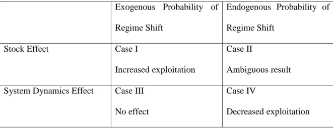
We summarize the differences between our results where regime shift leads to changes in system dynamics and the prior literature on stock collapse in Table 1. Regime shifts with changes in system dynamics (but no stock effect) do not cause a change in optimal
19
management by themselves (Case III). Only if management actions lead to changes in the probability of a regime shift (via changes in the state of the system) will the potential for regime shift lead to changes in optimal management (Case IV). In this case, optimal management is to become precautionary in the sense that a threat of future regime shift will cause managers to reduce current harvests and increase the stock of the resource. For climate change, this would mean that consideration of the potential of future regime shifts should cause a decrease in current emissions of greenhouse gases. In contrast, the potential for stock collapse itself causes a shift in optimal management towards more aggressive exploitation (Case I). With endogenous probabilities, management tends to become more precautionary, but whether this is sufficient to override the stock effect is ambiguous (Case II).
Table 1: Comparison of models and results
Exogenous Probability of Regime Shift
Endogenous Probability of Regime Shift
Stock Effect Case I
Increased exploitation
Case II
Ambiguous result System Dynamics Effect Case III
No effect
Case IV
Decreased exploitation
We have assumed that if the regime shift occurs, it is a once and for all shift. In reality, however, it is likely that there will be potential for the regime to shift back again to the original regime or for it to shift between a number of different regimes. In addition, there may be more than one threat process at work leading to the potential for multiple types of regime shift. Analyzing these possibilities implies a more complicated analysis with a series of nested Hamilton-Jacobi-Bellman equations with value functions characterizing the
20
different regimes. Doing so will change the results, of course, but not the logic that we find in our simple model above with only one potential regime shift. Similarly, a regime shift may be accompanied by a partial stock collapse which will lead to intermediate results, but again the logic of our analysis will remain.
Another potentially fruitful avenue for future research is to extend the model of uncertainty. Using a hazard rate is a very convenient approach and it captures many important features of the problem. This approach, however, does not allow for endogenous learning about probabilities of regime shift with additional experience or with active experimentation. Experimentation to learn about system dynamics can also influence optimal management (e.g., Walters and Holling 1990). Incorporating the option to learn is an important extension of the approach considered here. Finally, our model assumes constant prices and abstracts from costs that change with harvest or stock levels. Having a non-linear objective function in the control variable would make the model more difficult to solve. In principle such a model could be solved, at least numerically. We leave such extensions for further research.
References
V.I. Arnol’d, Geometrical methods in the theory of ordinary differential equations, Springer, New York (1988)
T. Aronsson, K. Backlund and K.-G. Löfgren, Nuclear power, externalities and non-standard Pigouvian taxes: a dynamic analysis under uncertainty, Environmental and Resource Economics 11(2), 177-195 (1998).
21
C. Azariadis, Self-fulfilling prophesies, Journal of Economic Theory 25, 380-396 (1981).
A.V. Banerjee, A simple model of herd behavior, Quarterly Journal of Economics 107(3), 797-817 (1992).
S. Bikhchandani, D. Hirschleifer and I. Welch, A theory of fads, fashion, custom and cultural change as information cascades, Journal of Political Economy 100(5), 992-1026 (1992).
W.A. Brock and C.H. Hommes, Heterogeneous beliefs and routes to chaos in a simple asset pricing model, Journal of Economic Dynamics & Control 22(8/9), 1235-1274 (1998).
W.A. Brock, C.H. Hommes and F.O.O. Wagener, More hedging instruments may destabilize markets, Journal of Economic Dynamics & Control 33(11), 1912-1928 (2009).
W.A. Brock and D. Starrett, Managing systems with non-convex positive feedback, Environmental and Resource Economics 26(4), 575–602 (2003).
N. Brozovic and W. Schlenker, Optimal management of an ecosystem with an unknown threshold, http://ssrn.com/abstract=990613 (2008).
S.R. Carpenter, Regime Shifts in Lake Ecosystems: Pattern and Variation, International Ecology Institute, Oldendorf (2003).
S.R. Carpenter, D. Ludwig and W.A. Brock, Management and eutrophication for lakes subject to potentially irreversible change, Ecological Applications 9(3), 751-771 (1999).
22
D. Cass and K. Shell, Do sunspots matter?, Journal of Political Economy 91(2), 193-227 (1983).
H.R. Clarke and W. J. Reed, Consumption/pollution tradeoffs in an environment vulnerable to pollution-related catastrophic collapse, Journal of Economic Dynamics & Control 18(5), 991–1010 (1994).
M.L. Cropper, Regulating activities with catastrophic environmental effects, Journal of Environmental Economics and Management 3(1): 1–15 (1976).
D. Grass, J. P. Caulkins, G. Feichtinger, G. Tragler and D. A. Behrens, Optimal control of nonlinear processes, Springer, Berlin (2008)
G. Gennotte and H. Leland, Market liquidity, hedging, and crashes, American Economic Review 80(5): 999-1021 (1990).
J. Gjerde, S. Grepperud and S. Kverndokk, Optimal climate policy under the possibility of a catastrophe, Resource and Energy Economics 21(3/4), 289-317 (1999).
M. Gladwell, The tipping point: how little things can make a big difference, Little, Brown and Company (2000).
23
C. Gollier, B. Jullien and N. Treich, Scientific progress and irreversibility: an economic interpretation of the ‘Precautionary Principle’, Journal of Public Economics 75(2): 229-253 (2000).
X. Guo, J. Miao and E. Morellec, Irreversible investment with regime shifts, Journal of Economic Theory 122(1), 37-59 (2005).
J. Hamilton, A new approach to the economic analysis of nonstationary time series and the business cycle, Econometrica 57(2), 357–384 (1989).
T.P. Hughes, A.H. Baird, D.R. Bellwood, M. Card, S.R. Connolly, C. Folke, R. Grosberg, O. Hoegh-Guldberg, J.B.C. Jackson, J. Kleypas, J.M. Lough, P. Marshall, M. Nyström, S.R. Palumbi, J.M. Pandolfi, B. Rosen and J. Roughgarden, Climate change, human impacts, and the resilience of coral reefs, Science 301, 929–933 (2003).
M.A. Janssen, J.M. Anderies and B.H. Walker, Robust strategies for managing rangelands with multiple stable attractors, Journal of Environmental Economics and Management 47(1), 140-162 (2004).
M. Kamien and N. Schwartz, Optimal maintenance and sale age for a machine subject to failure, Management Science 17(8), 495-504 (1971).
K. Keller, B.M. Bolker and D.F. Bradford, Uncertain climate thresholds and economic optimal growth, Journal of Environmental Economics and Management 48(1), 723–741 (2004).
24
T. Lauck, C.W. Clark, M. Mangel and G.R. Munro, Implementing the Precautionary Principle in fisheries management through marine reserves, Ecological Applications 8, S72-S78 (1998).
K.-G. Mäler, A. Xepapadeas and A. de Zeeuw, The economics of shallow lakes, Environmental and Resource Economics 26(4), 603–624 (2003).
K.-G. Mäler, C.-Z. Li and G. Destouni, Pricing resilience in a dynamic economy-environment system: A capital-theoretic approach, Beijer Discussion Paper 208 (2007).
E. Nævdal, Optimal regulation of eutrophying lakes, fjords and rivers, American Journal of Agricultural Economics 83(4): 972–984 (2001).
E. Nævdal, Optimal regulation of natural resources in the presence of irreversible threshold effects, Natural Resource Modeling 16(3), 305–333 (2003).
E. Nævdal, Dynamic optimization in the presence of threshold effects when the location of the threshold is uncertain with an application to a possible disintegration of the western Antarctic ice sheet, Journal of Economic Dynamics & Control 30(7), 1131-1158 (2006).
C. Perrings and B. Walker, Biodiversity, resilience and the control of ecological-economic systems: the case of fire-driven rangelands, Ecological Economics 22(1), 73-83 (1997).
25
G.D. Peterson, S.R. Carpenter and W.A. Brock, Uncertainty and the management of multistate ecosystems: An apparently rational route to collapse, Ecology 84(6), 1403–1411 (2003).
C. Raffensperger and J. Tickner (Eds.), Protecting public health and the environment: Implementing the Precautionary Principle, Island Press, Washington DC (1999).
W.J. Reed, The effects of the risk of fire on the optimal rotation of a forest, Journal of Environmental Economics and Management 11(2), 180-190 (1984).
W.J. Reed, Protecting a forest against fire: Optimal protection patterns and harvest policies, Natural Resource Modeling 2, 23-54 (1987).
W.J. Reed, Optimal harvesting of a fishery subject to random catastrophic collapse, IMA Journal of Mathematics Applied in Medicine & Biology 5(3), 215-235 (1988).
W.J. Reed, Optimal investment in the protection of a vulnerable biological resource, Natural Resource Modeling 3, 463-480 (1989).
W.J. Reed and H. Echavarria Heras, The conservation and exploitation of vulnerable resources, Bulletin of Mathematical Biology 54(2-3), 185-207 (1992).
D.S. Scharfstein and J.C. Stein, Herd behavior and investment, American Economic Review 80(3), 465-479 (1990).
26
M. Scheffer, The ecology of shallow lakes, Chapman and Hall, London (1997).
M. Scheffer, S. R. Carpenter, J. A. Foley, C. Folke and B.Walker, Catastrophic shifts in ecosystems, Nature 413, 591-596 (2001).
M. Spence and D. Starrett, Most rapid approach paths in accumulation problems, International Economic Review 16(2), 388–403 (1975).
Y. Tsur and A. Zemel, Uncertainty and irreversibility in groundwater management, Journal of Environmental Economics and Management 29(2), 149–161 (1995).
Y. Tsur and A. Zemel, Accounting for global warming risks: resource management under event uncertainty, Journal of Economic Dynamics & Control 20(6/7), 1289–1305 (1996).
Y. Tsur and A. Zemel, Pollution control in an uncertain environment, Journal of Economic Dynamics & Control 22(6), 967–975 (1998).
Y. Tsur and A. Zemel, Welfare measurement under threats of environmental catastrophes, Journal of Environmental Economics and Management 52(1), 421-429 (2006).
Y. Tsur and A. Zemel, Regulating environmental threats, Environmental and Resource Economics 39(3), 297-310 (2008).
C.J. Walters and C. S. Holling, Large-scale management experiments and learning by doing, Ecology: 71(6), 2060-2068 (1990).
27 Appendix 1
a) Constant hazard rate
In the first regime with carrying capacity K1, starting from stock levels that are higher
than s2, harvest levels h must maximize the expected value of the revenue
)), ( ( ) ( 2 0
τ
τ τ s V e dt t ph e−rt + −r∫
(A1)subject to stock dynamics with growth function G1. For a constant hazard rate λ we can
easily write this expected value as follows:
∫
∫
∞ − − − + 0 2 0 ))} ( ( ) ( {τ
τ
λ
e λτ τe rtph t dt e rτV s d (A2)or, by changing the order of integration,
, )) ( ( ) ( ) ( 0 2 ) ( 0
∫
∫ ∫
∞ − + ∞ − ∞ −τ
+λ
τ
τ
λ
e λτd e rtph t dt e r λτV s d t (A3) which leads to . ))} ( ( ) ( { 0 2 ) (∫
∞ + − + dt t s V t ph e r λtλ
(A4)The current value Pontryagin function for this problem reads as ). ) ( ( ) ( ) , , (s h ph V2 s G1 s h P
µ
= +λ
+µ
− (A5)Maximizing with respect to the harvest h yields that h = 0, if p < µ, h = ∞, if p > µ, and h is singular, if p = µ. If the optimal harvest is singular on a time interval, we have there the condition µ(t) = p for the co-state µ. From the co-state equation
)) ( ( ' ) ( )) ( ( ' ) ( ) ( ) (t r
λ
µ
tλ
V2 s tµ
t G1 s tµ
ɺ = + − − (A6)it follows that on such an interval
p s V r s G '( ) 2'( ) 1 = +λ−λ (A7)
28
for a constant s with h = G1(s). Case 1 and case 3 follow immediately.
b) Variable hazard rate
With the hazard function λ given by
t t t t t P t t ∆ ∉ ∆ + ∈ =∆lim→ ( {, )| {0, }) ) ( 0 τ τ λ (A8)
the probability S that no regime shift has occurred up to time t is given by = ∆ ∆ − = ∆ ∆ − =∆→
∏
∆→∑
i t i t i t t i t t tS( ) lim (1 ( ) ) limexp{ ln(1 ( ) )} 0 0 λ λ }, ) ( exp{ } ) ( exp{ lim 0 0 −
∑
∆ ∆ = −∫
=∆→ t i t λ i t t λ x dx (A9)so that the cumulative distribution function Sc for the time τ of the regime shift becomes
. 1 ) ( 1 ) ( ) ( = < = − = − −∫0 ( ) t dx x c e t S t P t S
τ
λ (A10)This yields as expected value of the revenue
∫ ∫
∞ − − + 0 2 0 ) ( ))} ( ( ) ( { ττ
τ
τ c r rt dS s V e dt t ph e (A11)or, by changing the order of integration,
, ) ( )) ( ( ) ( ) ) ( ( 0 2 0
∫
∫ ∫
∞ − ∞ − ∞ +τ
τ
τ
rt rτ c t c dS s V e dt t ph e dS or , ) ( )) ( ( ) ( 0 ) ( 2 0 ) ( 0 0∫
∫
∞ − − ∞ − − ∫ + ∫λ ττ
λ
τ
τλτ
d e s V e dt t ph e e xdx rt r xdx t (A12) which leads to . ))} ( ( ) ( ) ( { 0 2 )) ( ( 0∫
∞ + − + ∫ dt t s V t t ph e t dx x rλ
λ (A13)29 . 0 ) 0 ( ), ( ) ( , ) ( ) ( 0 = = =
∫
x dx q t t q t q tλ
λ
ɺ (A14)Assuming that the hazard rate λ is a function of the stock s, the current value Pontryagin function for this problem reads as
). ( ) ) ( ( )) ( ) ( ( ) , , , , (s q h e ph sV2 s G1 s h s P
µ
σ
= −q +λ
+µ
− +σλ
(A15)Maximizing with respect to the harvest h yields that h = 0, if e-qp < µ, h = ∞, if e-qp > µ, and h is singular, if e-qp = µ. If the optimal harvest is singular on a time interval, we have there the condition µ(t) = e-q(t)p for the co-state µ. From the co-state equation in µ
)) ( ( ' ) ( )) ( ( ' ) ( ))} ( ( ' )) ( ( )) ( ( )) ( ( ' { ) ( ) ( 1 2 2 ) ( t s t t s G t t s V t s t s V t s e t r t qt
λ
σ
µ
λ
λ
µ
µ
− − + − = − ɺ (A16) with p e t s p e t q t) ( ) q(t) ( ( )) q(t) ( =− − =−λ
−µ
ɺ ɺ (A17)it follows, after eliminating the co-state µ and multiplying with eq(t), that at each time t ). ( ' ) ( ' ) ( ' ) ( ) ( ) ( ' ) ( 0=
λ
s p+rp−λ
sV2 s −λ
s V2 s −pG1 s −eqσλ
s (A18) Differentiating this equation with respect to time t for a constant s yields). ( ) ( ) ( ) ( ' ) ( ) ( ' ) ( ) ( 0 () () t s t s t e s t s eqt
λ
σ
λ
− qtσ
λ
⇒σ
=−λ
σ
− = ɺ ɺ (A19)From this and the co-state equation in σ
))} ( ( )) ( ( ) ( { ) ( ) ( 2 ) ( t s V t s t ph e t r t
σ
qtλ
σ
= + − + ɺ (A20)it follows that at each time t
)). ( ) ( ( )) ( (r s e ph sV2 s q
λ
σ
λ
=− + + − (A21)Using this equation to eliminate eqσ from (A18) and substituting h = G1(s) finally leads to
)]. ( ) ( [ ) ( ) ( ' ) ) ( ' 1 )( ( ) ( ' 2 1 2 1 V s p r s G s r s p s V s r s G − + + − + = λ λ λ (A22)
30 Appendix 2
In this appendix, we prove a verification theorem for the value function V1 constructed in the
main part of the article. Recall that the function V1 satisfies the following properties: it is
continuous and at least piecewise continuously differentiable. Moreover, there are finitely many points 1 ) ( 1 ) ( 1 ) 1 ( 1 ) 1 ( 1 ) 0 ( 1 0=s ≤s ≤s ≤⋯≤s n ≤s n =K such that ( 1) ( ) 1 1 1 ( ) 1 1 ( ) ( ) 1 1 1 ( ) , if , ( ) , if , ( ) , if . i i i i i V s p s s s V s p s s V s p s s s − ′ > < < ′ = = ′ < < <
Only at the points s=s1(i), i=1,⋯,n−1, the function V1 may fail to be differentiable. It is
continuously differentiable everywhere else, satisfying there the Hamilton-Jacobi-Bellman equation . 0 ) ( max 2 1 1 1 1 0 = + − − + ′ − ≤ ≤h hm ph V V rV V G h
λ
λ
(A23)Note that the points 1()
i
s are precisely those points at which the function f , defined in the main text, satisfies for s in a neighbourhood of s1(i) that f(s)≤0 if s≤s1(i) and f(s)≥0 if
) ( 1
i
s
s≥ . It follows from this that the harvesting rule h* solving the maximisation in (A23) is of the form
( )
* ( 1) ( ) 1 1 * ( ) ( ) 1 1 * ( ) ( ) 1 1 ( ) 0, if , ( ) , if , ( ) ,if . i i i i i i M h s s s s h s G s s s h s h s s s − = < < = = = < <31 For s=s 1(i) there are two possibilities:
{
}
( )
* ( ) 1 1 * ( ) 1( ) 0, ,if is not differentiable at ,
( ) , otherwise. i M i h s h V s s h s G s = = =
In the first case, the decision maker is indifferent between two distinct actions; and such a point is called an indifference point (or Skiba point, or DNS(S) point: see Grass et al. (2008)).
We note that if s is the solution of the equation ) ( ) ( * 1 s h s G sɺ= −
with initial condition s(0)=s0, then
+ =
∫
− ( ( )) − ( ( )) ) ( 2 0 * 0 1τ
τ τ s V e dt t s h p e E s V rt rWe shall show that h*(s(t)) is the optimal harvesting schedule.
Theorem. Let h=h(t) be an admissible harvesting schedule, and let s=s(t) satisfy
0 ) 0 ( s s = and ) ( )) ( ( ) (t G1 s t h t sɺ = − a.e. Then
(
)
1 0 2 0 ( ) rt ( ) r ( ( )) V s ≥E∫
τe− p h t dt+e V s−ττ
(A24)and equality obtains if and only if )) ( ( ) (t h* s t h = a.e.
Proof. In the following, all harvesting schedules will be assumed to be admissible. We introduce
{
(1) (1) ( ) ( )}
1 , 1 , , 1 , 1 . n n s s s s Σ = ⋯32
and make the following fundamental observation. The subset of continuously differentiable harvesting schedules is dense in the set of all schedules, as is the smaller subset of continuously differentiable schedules for which
( ) 0 whenever ( ) .
h t′ ≠ s t ∈ Σ (A25)
Here s is stock evolution associated to the schedule h. The latter property is a consequence of Sard’s theorem (see e.g. Arnol’d, 1988).
Recall from appendix 1 that
. ) ( )) ( ( )) ( ( 0 2 )) ( ( 2 0 *
∫
0∫
− − = ∞ −∫ + + e ph s t dt+e V s e ph V dt E t dx x r r rt ττ
λλ
τ (A26)By the observation above, if there is a harvesting schedule for which (A24) is violated, then there is another continuously differentiable schedule h=h(t) satisfying (A25) which also violates (A24). Given this schedule, let s=s(t) be the stock evolution associated to it, and let * *( ( )).
t s h h =
For s=s(t)∉Σ, the function V1 is differentiable and the following equation obtains:
. ) ( ) ( 1 1 1 )) ( ( 1 )) ( ( 0 0 ′ − − + ∫ = ∫− + − + V r h G V e V e dt d t r x dx tr x dx
λ
λ λ (A27)All arguments (t) and s(t) are suppressed in this equation for readability. There is an increasing sequence
⋯
< < = 0 1 0 t t
such that s=s(t)∉Σ if t ≠tj, for any j. Note that since the elements of Σ are isolated, the sequence {tj} has no accumulation points. Integrating the identity (A27) from tj−1 to tj
33
(
)
1 0 0 0 1 ( ( )) ( ( )) 1 1 ( ( )) 1 1 1 ( ( )) ( ( )) ( ) ( ) . tj tj t j j r x dx r x dx j j t r x dx t e V s t e V s t e V G h r V dt λ λ λλ
− − − + − + − − + ∫ − ∫ ∫ ′ =∫
− − +Summing these expressions over all j yields then
. ) ( ) ( ) ( 0 1 1 1 )) ( ( 0 1 0 V G h r V dt e s V t dx x r
∫
∞ − + ′ − − + ∫ = − λλ
(A28)Adding equations (A26) and (A28) yields
. )) ( ( ) ( )) ( ( ) ( 0 2 1 1 1 1 )) ( ( 0 1 2 0 0
∫
∫
∞ − + − − − ′ + − − + ∫ = − + dt h G V rV V V h p e s V s V e dt t h p e E t dx x r r rtλ
λ
τ
λ τ τ (A29)As h* solves the Hamilton-Jacobi-Bellman equation, subtracting equation (A23) from equation (A29) yields
(
)
. ) ( )) ( ( ) ( 1 0 * 1 )) ( ( 0 1 2 0∑ ∫
∫
− − − ′ ∫ = − + + − − − j t t dx x r r rt j j t dt h h V p e s V s V e dt t h p e E λ τ ττ
Now, if tj−1 <t <tj, then either V1′ > p and 0=h* ≤h, or V1′ < p and hm =h* ≥h. In both cases it follows that
0 ) )(
(p−V1 h* −h ≤
for almost all t > 0. Consequently
, 0 ) ( )) ( ( ) ( 2 1 0 0 − ≤ − + −