of Planar Graphs
Ittai Abraham
1, Shiri Chechik
2, Robert Krauthgamer
∗3, and
Udi Wieder
31 VMware Research, Palo Alto, CA, USA,{iabraham,uwieder}@vmware.com
2 Tel-Aviv University, Tel-Aviv, Israel, shiri.chechik@gmail.com
3 Weizmann Institute of Science, Israel,robert.krauthgamer@weizmann.ac.il
Abstract
We investigate the problem of approximate Nearest-Neighbor Search (NNS) in graphical metrics: The task is to preprocess an edge-weighted graphG= (V, E) onmvertices and a small “dataset” D⊂V of sizenm, so that given a query pointq∈V, one can quickly approximatedG(q, D)
(the distance fromq to its closest vertex inD) and find a vertexa∈Dwithin this approximated distance. We assume the query algorithm has access to a distance oracle, that quickly evaluates the exact distance between any pair of vertices.
For planar graphsGwith maximum degree ∆, we show how to efficiently construct a compact data structure – of size ˜O(n(∆ + 1/)) – that answers (1 +)-NNS queries in time ˜O(∆ + 1/). Thus, as far as NNS applications are concerned, metrics derived from bounded-degree planar graphs behave as low-dimensional metrics, even though planar metrics do not necessarily have a low doubling dimension, nor can they be embedded with low distortion into`2. We complement our algorithmic result by lower bounds showing that the access to an exact distance oracle (rather than an approximate one) and the dependency on ∆ (in query time) are both essential.
1998 ACM Subject Classification F.2 Analysis of Algorithms and Problem Complexity
Keywords and phrases Data Structures, Nearest Neighbor Search, Planar Graphs, Planar Met-rics, Planar Separator
Digital Object Identifier 10.4230/LIPIcs.APPROX-RANDOM.2015.20
1
Introduction
In the Nearest Neighbor Search (NNS) problem, the input is a dataset D ={p1, . . . , pn}
containingn points that lie in some large host metric space (M, d). These points should be preprocessed into a data structure so that given a query pointq∈M, the dataset point pi∈D closest toqcan be reported quickly. The scheme’s efficiency is typically measured by
the space complexity of the data structure and the time complexity of the query algorithm. NNS is a fundamental problem with numerous applications, and has therefore attracted a lot of attention, including extensive experimental and theoretical analyses. Often, finding the exact closest neighbor is relaxed to finding an approximate solution, called (1 +)-NNS, where the goal is to report a dataset pointpi∈Dsatisfyingd(q, pi)≤(1 +) min{d(q, pj)|pj∈D}.
Previous work on NNS has largely focused on the case where the host metric is`p-norm for
somep, typically`1or`2, over M =Rm for some dimensionm >0. In this common setting, exact NNS exhibits a “curse of dimensionality” – either the space (storage requirement) or
∗ Work supported in part by a US-Israel BSF grant #2010418 and an Israel Science Foundation grant
#897/13.
© Ittai Abraham, Shiri Checik, Robert Krauthgamer, and Uli Wieder; licensed under Creative Commons License CC-BY
18th Int’l Workshop on Approximation Algorithms for Combinatorial Optimization Problems (APPROX’15) / 19th Int’l Workshop on Randomization and Computation (RANDOM’15).
Editors: Naveen Garg, Klaus Jansen, Anup Rao, and José D. P. Rolim; pp. 20–42 Leibniz International Proceedings in Informatics
the query time must be exponential in the dimension – which provides a strong motivation to study approximate solutions. When the dimension m is constant, known (1 +)-NNS algorithms achieve almost linear space and a polylogarithmic query time; but when the dimension is logarithmic (inn), all known algorithms, including approximate ones, require (in the worst-case) either a super-linear space or a polynomial query time.
While the `p-norm setting captures many applications, certain data types cannot be
embedded (with low distortion) intoRm, and it is therefore desirable to consider other metric
spaces. However, the notion of dimensionality is not well-defined for general metrics, and it is unclear a-priori what type of internal structure suffices for efficient approximate NNS algorithms. A notable example of such an approach, initiated by [22, 17, 18], is the study of NNS in general metric spaces assuming the algorithm has access to a distance oracle, i.e., that the distance function can be evaluated in unit time; their motivation was drawn from the analysis of computer networks, where distances are derived from a huge graph (rather than by a norm or another simple function of the vertex names). It is known [18, 19, 8, 15, 12] that if the metric space restricted to thendataset points has a bounded doubling dimension, then (1 +)-NNS can be solved with near-linear space and polylogarithmic query time.
1.1
Our Results
We look at another family of metric spaces, those derived by way of shortest paths from a graph with positive edge weights. Similarly to [22, 17, 18], we assume the NNS algorithm has access to a distance oracle.
As a motivating application consider the case where the graph represents a road network, say of the continental United States. Even though this graph has tens of millions of nodes, extremely efficient exact distance oracles have been built for it (see [14, 6, 2]). Now suppose we wish to find the nearest shop from a collection like the set of all Starbucks shops, which currently has roughly 12,000 locations in the US. This means we want to design a compact application (e.g., mobile app) that has access to a generic server (like google maps). While the server could use much larger space (but cannot be customized to support specialized operations like NNS), the application must be very efficient in terms of query time and space, and thus our goal is to build an NNS data structure whose efficiency depends on the significantly smaller number of shops (n=|D|in our notation).
Our main result is that in planar graphs of bounded degree, (1 +)-NNS can be solved using near-linear space and polylogarithmic query time. Thus, bounded-degree planar metrics exhibit “low-dimensional” behavior, even though they do not necessarily have a low doubling dimension, nor can they be embedded with low distortion into`2. This phenomenon, namely, that the restricted topology of planar graphs maintains some of the geometric structure of the Euclidean plane, is known in other contexts like compact routing and TSP, but here we show it for the first time in the context of NNS.
ITheorem 1. Let(M, d)be a metric derived from a plane graph of maximum degree∆>0 with positive edge weights, and let > 0. Then every dataset D⊂M of size n=|D| can be preprocessed into a data structure of sizeO(−1nlognlog|M|+n∆ log2n)words, which can answer(1 +)-NNS queries in time O((−1log logn+t
DO) lognlog|M|+ logn·∆tDO),
assuming the distance between any two points inM can be computed in timetDO.
The data structure’s size is measured in words, where a single word can accommodate a point inM or a (numerical) distance value. The term plane graph refers to a planar graph accompanied with a specific drawing in the plane.
Theorem 1 makes two assumptions, that there is a bound on the maximum degree, and that the data structure has access to an exact distance oracle. We further show (in Section 4) that both of these assumptions are necessary. Roughly speaking, we prove that if the degree is large, or if the distance oracle is approximate, the graph could contain symmetries that only a large number of accesses to the distance oracle could break.
IRemark. We cannot dispose of the maximum degree assumption by “vertex splitting”, where a high-degree vertex is replaced with a binary tree with zero edge weights, because we assume access to a distance oracle forG(but not necessarily for a modified graphG0), since the distance oracle models a generic server. For the same reason, we cannot make the usual assumptions thatGis triangulated or perturb the pairwise distances to be all distinct.
1.2
Related Work
Our model of NNS for a datasetD embedded inside a (huge) graphGis related to vertex-sparsification of distances [20], where the goal is to construct a small graphG0that (i) contains all the dataset pointD (called terminals here) and furthermore maintains all their pairwise distances; and (ii) is isomorphic to a minor ofG.
Here is another interesting related problem that is open: Given only the distances between a datasetD, find in polynomial time aplanar host graph Gthat containsD and realizes their given pairwise distances (perhaps even approximately).
A key difference of our NNS model from these two problems is that the vertices outside of Dare actually used explicitly as query points. However, one may hope for some connections, at least at a technical level.
1.3
Techniques
At a very high level, our algorithm is reminiscent of the classicalk-d tree algorithm for NNS due to Bentley [7], as it partitions the graph recursively using separators that split the current dataset in an approximately balanced manner. Whilek-d trees use hyperplanes as separators of the host space, for planar metrics we use shortest-paths as separators (see [23, 3, 1, 13]). This recursive partitioning process can be described as creating a “hierarchy” treeT, whose nodes correspond to “regions” in the metric space, and every leaf node represents a region with at most one dataset point; in our graphical case, every region is an induced subgraph ofG. Given a query pointq, one often uses a top-down algorithm to identify the leaf node in the hierarchy treeT that “contains”q, by tracing the location ofqalong the recursive partitioning, a process that we call the “zoom-in” phase. While this phase is trivial ink-d trees, and simple in bounded treewidth graphs (see Section 1.4), it is quite non-trivial in planar graphs, as explained below.
The key observation that completes thek-d tree algorithm is that once the tree leaf node containingqhas been located, the nearest neighbor ofqmust lie “near the boundary” of one of the regions along the tree path leading to this leaf. Thus, all we need to store is just the separators themselves and the dataset points near them.
In planar graphs, this master plan has two serious technical difficulties. First, the separators themselves are too large to be stored explicitly. Recalling that the separators consist of shortest paths, we can employ the known trick [23, 3, 1, 13] of using a carefully chosen “net” to store them within reasonable accuracy, but since we actually need a net of all nearby dataset points, our solution is more involved and roughly uses a net of nets. Second, tracing the path toqalong the hierarchy tree is a major technical challenge because our storage is proportional ton=|D|, while the separator size could be much larger, even
linear in|M|. Our solution is to store just enough auxiliary information to identify at each level of the tree a few (rather than one) potential nodes, which suffices to “zoom-in” towards a small set of leaves that one of them containsq. The construction is presented in Section 2.
As a warm-up to the main result, we demonstrate our approach on the much simpler case of graphs with a bounded treewidth, where our algorithm solves NNSexactlyusing a standard tool of vertex separators of bounded size. This is only an initial example how NNS algorithms can leverage topological information, and the case of planar graphs is considerably more difficult — our algorithm uses a path separator, whose size is not bounded, and consequently solves NNSapproximately (within factor 1 +).
1.4
Warmup: Bounded Treewidth Graphs
ITheorem 2. LetDbe a dataset ofnpoints in a metric(V, d)derived from an edge-weighted graph of treewidthw≥1 and maximum degree∆>0. Then D can be preprocessed into a data structure of sizeO(∆wn)words, which can answer (exactly) nearest neighbor search queries in timeO(∆wlogn·tDO), assuming the distance between any two points in V can be
computed intDO steps.
We assume for simplicity of exposition that an optimal tree decomposition is given to us; otherwise, it is possible to compute in polynomial time a tree decomposition of width O(wlogw) [5] (or for fixedw, one of the algorithms of [9, 10]).
We use the following well-known property of bounded treewidth graphs: Given a set X ⊂V, we can efficiently find aseparator S ⊂V of size |S| ≤w+ 1 whose removal breaks Ginto connected componentsV1, V2, . . .such that|Vi∩X| ≤ |X|/2 for alli. (The separator
can be found by picking a single suitable node in the tree decomposition, and the width bound implies the bound on the separator size, see e.g. [11, Lemma 6].) It follows that inG, every path fromVi to Vj fori6=j, must intersect the separatorS.
The preprocessing phase
Given a datasetD={p1, . . . , pn}, recursively compute a partition (using the above property)
with respect to the dataset points in the current component (i.e., D∩V0 where V0 ⊆V denotes the current component), until no dataset points are left (they were all absorbed in the separators). It is easy to see that the depth of the recursion tree isO(logn), and the number of separators used (non-leaf nodes in the recursion tree) is at mostO(n), each with at mostw+ 1 nodes. The data structure stores all the separators explicitly arranged in the form of their recursion tree. In addition, for each vertexuin any of these separators, it stores the following meta-data:
All the neighbors (at most ∆) of u, along with the index of the partVi to which they
belong.
A dataset point that is closest tou, i.e., argminp∈Dd(p, u), breaking ties arbitrarily. The total number of vertices in all the separators is at mostO(nw) and the meta-data held for every separator vertexuis of size O(∆), hence the total size isO(∆wn) words. The query phase
We first argue that given a query pointq∈V and a separatorS, it is possible to check, using the meta-data stored in the preprocessing phase, which partVi containsq. This would imply
that we can trace the path along the recursion tree all the way down to the last component containingq, a process that was mentioned before as the “zoom-in” phase. Indeed, finding
thisViis done by finding a vertexu∈Sthat is closest toq, this task takes at most|S|=w+ 1
distance queries. Ifu=qwe are done. Otherwise, computeu’s neighbor that is closest toq, namely,v= argmin{d(q, v)|(v, u)∈E}, which takes another ∆ distance queries. Observe thatqmust lie in the same partVi asv, because the shortest between these two vertices
does not intersectS.
The next step after the zoom-in process is to find the nearest neighbor itself. LetS0 be the union of all the vertices in all the separators encountered during the zoom-in onq. It is easy to verify the following two facts:
|S0| ≤O(wlogn).
There existsu∈S0 that lies on the shortest-path betweenqand its nearest neighbor in the datasetD. Soq anduhave the same nearest neighbor.
Recall that the vertices inS0 along with all their nearest neighbors are stored explicitly in the data structure, and they can be “compared” againstqusing a distance oracle. Hence, it is possible to findq’sexact nearest neighbor in timeO(∆wlogn), assuming access to a distance oracle. This proves Theorem 2.
IRemark. Both the “zoom-in” phase and the calculation of the nearest neighbor itself were made easy by the fact that we stored all the separators explicitly in the data structure. Planar graphs onmnodes have separators of size O(√m), but in our modelmn, and thus storing the separators explicitly is prohibitively expensive.
2
Planar Graph Metrics
In this section we start proving Theorem 1. LetG= (M, E) be a connected planar graph with positive edge weightsω:E→R+, and letD⊆M be the dataset vertices. We denote n=|D|,m=|M|, and ∆ is the maximum degree inG. Assume the minimal edge weight is 1, and letDiam be the diameter of the graph. We usedG(·,·) to denote the shortest path distance inG, and assume it can be computed in timetDO e.g., by having access to a
distance oracle.
We shall start with the case where shortest paths inGare unique, as it simplifies technical matters considerably. A common workaround to this uniqueness issue is to perturb the edge weights, but this solution isnot applicable in our model of a black-box access to the distance functiondG(·,·), because its implementation could potentially exploit ties (e.g., by assuming all distances are small integers). The general case is sketched in Section 3.
It is worth pointing out that our algorithm relies on machinery developed in [1] to recursively partition a planar graphG, which relies in turn on a two-path planar separator. Unlike many algorithms for planar graphs, which use existence ofsmall separators, this machinery, described in detail in Section 2.1, uses the fact that the separators are shortest paths, and therefore could be represented succinctly, even if they are large. While this idea had been used before, applying it in the context of NNS (and providing matching lower bounds) requires a considerable amount of technical novelty, as described in Section 2.2.
2.1
Building the Hierarchy tree
T
Preprocessing algorithm, step 1. The algorithm fixes some vertex s∈ M. It then con-structs a shortest-path treeT rooted ats∈M by invoking Dijkstra’s single-source shortest-path algorithm froms.
Two-path planar separator. We use a version of the well-known Planar Separator Theorem by Lipton and Tarjan [21], where the separator consists of two paths in the shortest-paths
treeT ofG. In the specific version stated below, we are only required to separate a subset U ⊂ M, and the balance constraint refers to a subsetW ⊂ U. As usual, G[U] denotes the subgraph of G induced onU ⊂ M(G). We apply this theorem recursively using the same shortest-paths treeT. An additional concern for us is that this tree is too large to be stored entirely (it spans all nodes M), hence our algorithm will store partial information that suffices to efficiently perform the Zoom-In and Estimating the Distance operations.
Given a connected planar graph G, we assume throughout it is a plane graph, i.e., accompanied by a specific drawing in the plane, and that it is already triangulated. We let the new edges introduced by the triangulation have infinite weight (hence they do not participate in any shortest-path). While the triangulation operation may increase the maximum degree, it will not affect our runtime bounds (which depend on ∆), because our runtime bounds depend on the maximum degree in the treeT, which contains only edges from the original graph (and not from the triangulated one).1
For a rooted spanning tree ˜T ofG, define theroot-path of a vertexv∈M in this tree, denoted ˜Tv, to be the path in the tree ˜T connecting v to the root. (We use here ˜T for
generality, but will soon instantiate it with the tree T constructed in step 1.) The next theorem has essentially the same proof as of [21, Lemma 2]. It is particularly convenient for a recursive application, whereU ⊂M is the “current” subset to work on, yet Gand the tree
˜
T remain fixed through the recursive process. It shows that each set could be partitioned using a cycle which composed of two paths in the shortest path tree, plus an edge called the separator edge. We remark thatG[U] is not required to be connected.
ILemma 3([21]). Given a triangulated plane graphG= (M, E), a rooted spanning tree T˜ of G, a subset U ⊂M, and a vertex subset W ⊆U, one can find in linear time a non-tree edge (u, v)∈E(G)\E( ˜T)such that the cycleT˜u∪T˜v∪ {(u, v)} is a vertex-separator in the
following sense: U\( ˜Tu∪T˜v)can be partitioned into two subsets U1 and U2 such that (i) each ofU1∩W and U2∩W is of size at most 2|W|/3; and (ii) all paths from a vertex in U1 to a vertex inU2 intersectT˜u∪T˜v at a vertex.
Preprocessing algorithm, step 2. We invoke the algorithm of Lemma 3 recursively to construct a “hierarchy” tree T as follows. Each node µ in T corresponds to a triple
hG(µ), D(µ), e(µ)ithat records an invokation of Lemma 3 on G: G(µ) records the induced subgraph used asG[U];
D(µ)⊂D records the subset of data points used asW;
the treeT constructed in step 1 is used as ˜T (the same tree for allµ); and e(µ) records the edge ofGobtained by this invokation.
The root ofT corresponds tohG, D, e0iwheree0 is the edge obtained by invoking Lemma 3 withU =M,W =D. Consider now some nodeµinT, and letU1andU2be the two subsets ofU obtained from the corresponding invokation of Lemma 3 onG(µ) andD(µ). The two children ofµin the tree, denotedµi fori= 1,2, correspond, respectively, to the invokations
of Lemma 3 on the induced subgraphsG(µi) =G[Ui] with the setsD(µi) =Ui∩D. The
recursion stops at a nodeµif the corresponding G(µ)∩D=∅.
Structural properties of the hierarchy tree T. We need several definitions and proofs from [1], which are repeated here for completeness. For a node µ ∈ T, let the level of
1 One can also triangulateGwhile increasing its maximum degree by at most a constant factor [16,
u 2 v u 2 z v z R 1 1 2 2 z v z R 1 1 2 u R v2 u2 1 1 root(T) 3 R 4 R root(T) 1 2
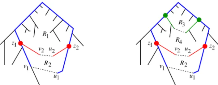
Figure 1 An illustration of apices and frames. The left figure shows the tree T using solid edges. The first separator-edge, at the hierarchy’s root, is the dashed edge (v1, u1). LetRbe the
corresponding cycle’s interior region. This regionRhas a separator-edge (v2, u2). The cycle-separator
of this regionR is the union of the two cycles defined by (v1, u1) and by (v2, u2). The apices ofR
are labeledz1 andz2.
The right figure then shows what happens in regionR1; the separator-edge is a green dashed line,
and the new apices are green circles. The frame ofRis the subgraph colored blue. The frame ofR2
contains all red and some blue edges. Note that all edges in the first separatorTv1∪Tu1 belong to
the frame of only one ofR1 andR2.
µ, denoted Level(µ), be the number of edges in T from µ to the root of T. Clearly, 0≤ Level(µ) ≤1 + log3/2n ≤ 2 logn. We now associate with each node µ of T three subgraphs ofG. First, define theclusterofµto be
Cluster(µ) :=G(µ).
Second, define the cycle-separator of µ recursively as follows. Ifµ is the root ofT, then
Cycle-Sep(µ) :=Tu∪Tv∪ {(u, v)}. Otherwise, letµ0 be the parent ofµinT, and let Cycle-Sep(µ) :=Cycle-Sep(µ0)∪Tu∪Tv∪ {(u, v)}.
Third, define theseparator ofµto be the subgraph of Cycle-Sep(µ) induced by the edges ofT, formally,
Sep(µ) :=Cycle-Sep(µ)∩E(T).
IObservation 4. For every µ, the subgraph Sep(µ)is a subtree of T containing its roots.
IObservation 5. For everyµ(other than the root) and its parentµ0, the vertices ofSep(µ0) separateCluster(µ)from the rest of G. This is immediate from Lemma 3.
Define the homeof a vertex x∈M, denotedHome(x), as the nodeµofT of smallest level such thatxbelongs toSep(µ).
Define theapicesof a nodeµ, denotedApices(µ), as the set of vertices inCycle-Sep(µ) that have degree≥3; see Figure 1 for an illustration. The apices ofµturn out to be a key enabler of our solution. As we show below, there are very few apices per region and they concisely represent the topological connections between nearby regions (note that degree 2 vertices ofCycle-Sep(µ) simply form paths between pairs of apices and topologically each such path can be contracted into an edge)
Thenew apicesofµare defined as follows. Ifµis the root ofT, thenNewApices(µ) :=
Apices(µ); otherwise, letNewApices(µ) :=Apices(µ)\Apices(µ0), whereµ0is the parent of µ in T. Intuitively, the new apices of µ are the vertices where the separator of µ “disconnects" from its parent separatorµ0.
ILemma 6([1]). For everyµwe have |NewApices(µ)| ≤2.
We next define the frameof a nodeµ, which is, loosely speaking, a small subgraph of
Sep(µ0) that separatesCluster(µ) from the rest ofG. Formally, ifµis the root ofT, then
Frame(µ) is the empty graph. Otherwise, letµ0 be the parent of µ, and letFrame(µ) be the subgraph ofSep(µ0) induced by the verticesxinSep(µ0), which can be connected to (some vertexz in)Cluster(µ) by a path whose internal vertices (i.e., all butx, z) are all inSep(µ0)\Apices(µ0). By construction, a path connecting a vertex ofCluster(µ) to a vertex outside the cluster has to intersectFrame(µ).
The region ofµ, denoted Reg(µ), is the subgraph of Ginduced by all the vertices of
Cluster(µ)∪Frame(µ).
ILemma 7([1]). For every level`≥0inT, every edge e∈E belongs to the frame of at most two nodesµ for whichLevel(µ) =`.
2.2
Finding the Query’s Region
Our goal is to find for every level `≤Level(Home(q)) the region that contains the query q. (There is exactly one such region, because q is not in the separator.) We provide a slightly weaker guarantee that is sufficient for our needs: we show how to compute for every ` = 0,1, . . . ,2 logn a set A`(q) of at most two regions, such that whenever `≤Level(Home(q)), the setA`(q) contains the region containingq.
Query Algorithm for Region Finding (Zoom-In). For a nodeµ of T, let its near-apices be the set of all edges incident to the apices ofµor tos(the root of the shortest path tree T); formally,N A(µ) :={(y, x)∈E|x∈Apices(µ)∪ {s}}, where we view each (y, x) as an ordered pair.
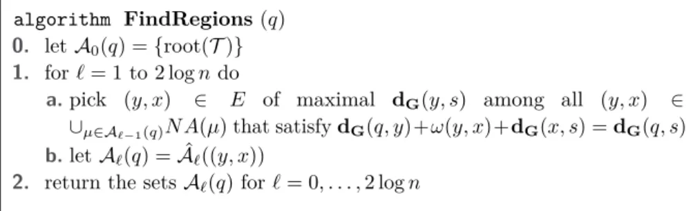
The query algorithm computes A`(q) iteratively for level ` = 0,1, . . . ,2 logn. After initializingA0(q) ={root(T)}, it computes the next setA`(q) usingA`−1(q) as follows. Find the edge (y, x) for whichyis furthest away froms, among all edges (y, x)∈ ∪µ∈A`−1(q)N A(µ)
such that (y, x) is on the shortest path from q to s. Here, we treat (y, x) as an ordered pair, and insist thaty appears beforexalong the path fromq tos, or equivalently, that dG(q, y) +ω(y, x) +dG(x, s) =dG(q, s), which can be checked using only a constant number of distance oracle queries. Notice such (y, x) always exists, because the rootsis an apex and one of its incident edges is on the shortest paths fromqtos. Next, letA`+1(q) be the set of regions at level`+ 1 that contain the edge (y, x), which we prepare in advance (during the preprocessing phase) as the set ˆA`0((y, x)). Finally, proceed to the next iteration.
algorithm FindRegions(q)
0. letA0(q) ={root(T)} 1. for`= 1 to 2 logndo
a.pick (y, x) ∈ E of maximal dG(y, s) among all (y, x) ∈ ∪µ∈A`−1(q)N A(µ) that satisfydG(q, y)+ω(y, x)+dG(x, s) =dG(q, s) b.letA`(q) = ˆA`((y, x))
2. return the setsA`(q) for`= 0, . . . ,2 logn
ILemma 8. For every level `≤Level(Home(q)), the query vertex qbelongs to a region in{Reg(µ)|µ∈ A`(q)}.
Proof. The proof is by induction on`. For `= 0, we initializedA0(q) ={root(T)}and the corresponding regionReg(root(T)) is the entire graphG, henceq∈Reg(root(T)). Assume now the claim holds for level`and consider level`+ 1. Let (y, x) be the edge of maximal dG(s, y) among all edges in∪µ∈A`(q)N A(µ) that lie on a shortest path fromqtos.
Supposeq∈Rfor a regionRat level`+ 1, and let us show thatR∈ A`(q). Letµbe the
corresponding node inT, i.e.,Reg(µ) =R, and letµ0 be the parent node ofµinT. Observe thatq∈Reg(µ0), becauseq must be inCluster(µ) (rather than Frame(µ)), and all such vertices are inside the region of the parentµ0. Thus by the induction hypothesisµ0∈ A`(q).
LetP(q, s) be the unique shortest path fromqtos, and letz be the first vertex along this path (furthest from the roots) which is inApices(µ0). Suchz exists (because the root sis an apex) and is not the first vertex on the path (becauseqitself is not an apex), so let z1be vertex precedingz on this path.
We now claim that (z1, z) is exactly the edge (y, x) chosen. Indeed, the edge (z1, z) satisfies the two requirements (it is inN A(µ0) and on the shortest path from q to s) by definition, and moreover,zwas chosen to that it is closest toqand thus furthest from s.
The claim implies, by the construction ofzas the first apex onP(q, s), that the regionR containingqalso contains the edge (z1, z) = (y, x), which means that the algorithm will add
R=Reg(µ) toA`+1(q). J
2.3
Estimating the Distance
Once we have located the region ofq, we would like to complete the nearest neighbor search. Lett∗∈D be the closest dataset point toq, and letP(q, t∗) be the shortest path fromq to t∗, then we would like to approximate the length ofP(q, t∗). Since we locatedq’s region, we can follow the path from the root of the treeT toq’s region. We observe that at some tree nodeµwe reach a situation whereP(q, t∗) intersects Frame(µ). Indeed, the region at the root of the tree contains bothqandt∗; however, at the leafµof the tree, the region contains qand either (i) does not contain t∗, in which case the path P(q, t∗) connects a vertex in
Cluster(µ) to one outsideCluster(µ), and thus must intersectFrame(µ); or (ii) it does
containt∗, but only in its frame and not in its cluster (becauseCluster(µ)∩D=∅), in which caset∗ is itself in the intersection.
If the query procedure could identify a vertexv on this intersection betweenP(q, t∗) and
Frame(µ), then it could solve finding the nearest neighbor problem for q by finding the nearest neighbor ofvand reporting the exact same vertex (and this holds also for approximate nearest neighbor). This is exactly the approach taken in our warmup, the bounded treewidth case, where the preprocessing phase stores for every separator vertex its nearest neighbor inD, and the query procedure just considers all the separator vertices in all the regions encountered during the zoom-in process forq.
However, in the planar graph setting, the number of vertices on a single separator may be arbitrarily large (compared ton). So we must exploit the separator’s structure as the union of a few shortest paths. At a very high level, our solution is to carefully choose net-points on the boundary of each region, and only for these net-point we store their nearest neighbor in D. The challenge is to choose the net-points in such a way that (i) for at least one “good” net-point in the sense that the distance fromqthrough the net-point and then toD (i.e., to the nearest neighbor of this net-point) is guaranteed to approximate the optimal NNS answer; and (ii) the query procedure can examine very few net-points (compared to the total number of net-points stored, which is linear inn) until one of these good points is found.
Before describing the algorithm in more detail, let us introduce some useful notations. For a vertexc on a pathP and a distanceρ0>0, letP(c, ρ0) be all nodes inP at distance at most ρ0 from c. LetN(P, c, ρ, ρ0) be a set of nodes in P(c, ρ0) such that every node in P(c, ρ0) has a node inN(P, c, ρ, ρ0) at distance ρand every two nodes inN(P, c, ρ, ρ0) are at distance at leastρfrom one another (this set can be obtained by considering all nodes on the pathP(c, ρ0) from endpoint of the path to another and adding toN(P, c, ρ, ρ0) every node that does not have yet a node inN(P, c, ρ, ρ0) at distanceρfrom it). For a shortest pathP and a nodev, let
Ni(v, P) :=N(P, cv,2i/32,2i+1),
and
N(v, P) := [ 0≤i≤log (nDiam)
Ni(v, P),
wherecv is the vertex in P closest tov.
For a tree nodeµ∈ T such thate(µ) = (u, v), we letN(Tu) :=∪w∈Cluster(µ)∩DN(w, Tu),
and similarly for N(Tv). (Formally, it depends also on µ, but we suppress this.) For a
shortest pathP fromsto some vertexf, letN(P, d1, d2) to be a vertex inN(P) as follows. If d2 >dG(s, f) then N(P, d1, d2) :=f. If d1 <0 then N(P, d1, d2) :=s. Otherwise let N(P, d1, d2) be the vertexx∈N(P) with minimaldG(x, s) among all verticesxsatisfying d1≤dG(x, s)≤d2; if no such vertex xexists, setN(P, d1, d2) :=null. For a tree nodeµ, letP(µ) ={Tu} ∪ {Tv} wheree(µ) = (u, v).
Preprocessing. Let us describe the additional information stored by our data structure. For every nodeµ, where we denote (u, v) =e(µ), store the setsN(Tz) for allz∈ {u, v}. In
addition, construct a range reporting data structure onN(Tz) according to the distance from
s. Namely, a data structure that given two distancesd1, d2 returns inO(log logn) time a vertexx∈N(Tz) withdG(x, s)∈[d1, d2] that has minimaldG(x, s) among all such vertices, or returns null if no such vertex exists. Observe that the range reporting data structure on N(P) makes it possible to findN(P, d1, d2) inO(log logn) time [4].
In addition, for every nodeµ, level`∈ {1, . . . ,2 logn}and apexx∈NewApices(µ), store
for every edgeeincident to xthe set ˆA`(e) ={µ∈ T |e∈E(Reg(µ))andLevel(µ) =`}, namely, the set of level`tree nodesµfor whichebelongs to their region (recall there are at most two such nodes). The algorithm also stores the numberOT(v) for every vertex vthat
is a neighbor of an apex of some nodeµ∈ T (for all apices).
For every tree nodeµ the algorithm stores an indicatorIL(µ) ifµis a leaf in T. Note that ifµis a leaf inT then its cluster contains at most one dataset point, denoted byD(µ). The algorithm also stores the dataset pointD(µ) in caseµis a leaf.
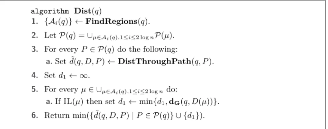
Distance Query. The distance query given a vertexqis performed as follows. (See Figure 3 for a pseudo-code description.) The algorithm starts by invoking ProcedureFindRegionsto obtain the sets{Ai(q)} for 1≤i≤2 logn, where each setAi(q) contains at most two nodes of leveli inT such thatqbelongs to the region of at least one of them. The algorithm then iterates on all path separators P inP(q) =∪1≤i≤2 logn∪µ∈Ai(q)P(µ). For a pathP ∈ P(q), letµ(P) be the node such thatP ∈ P(µ). For each such path separatorP, the algorithm invokes ProcedureDistThroughPath to estimatedG(q, D∩Cluster(µ(P)), P), namely, the length of the shortest path fromqto some vertex inD∩Cluster(µ(P)) among all such paths that go through some vertex inP. Let ˜d(P, q, D) be the estimated distance returned by this invokation of ProcedureDistThroughPath. In addition, the algorithm iterates over
algorithm Dist(q)
1. {Ai(q)} ←FindRegions(q).
2. LetP(q) =∪µ∈Ai(q),1≤i≤2 lognP(µ).
3. For everyP ∈ P(q) do the following:
a.Set ˜d(q, D, P)←DistThroughPath(q, P).
4. Setd1← ∞.
5. For everyµ∈ ∪µ∈Ai(q),1≤i≤2 logndo:
a.IfIL(µ) then setd1←min{d1,dG(q, D(µ))}.
6. Return min({d˜(q, D, P)|P ∈ P(q)} ∪ {d1}).
Figure 3Our main algorithm for estimating the distance between a given query vertexqand the closest data point to it inD.
algorithm DistThroughPath(q, P)
1. found=false.
2. Setp←s.
3. While (found=false)
a.Let ˜d=dG(p, q).
b.Find an ˜d/8-netS0 onN(P)∩P(p,2 ˜d).
c.Setpto be the vertex inS0∪ {p}such thatdG(q, p) is minimal.
d.IfdG(q, p)>d/˜2 then setfound=true.
4. Forifrom 1 to lognM do the following.
a.Find an 2i/8-netSionN(P)∩P(p,2i+3).
b.Set ˜d(q, D, P)ito be the minimal distancedG(q, x) +dG(q, D) forx∈Si.
5. Set ˜d(q, D, P) to be the minimal distance ˜d(q, D, P)i.
6. Return ˜d(q, D, P).
Figure 4A procedure for estimatingdG(q, D, P), which is the minimum length of a path from a
given query vertexqto some vertex inDamong all such paths that go through some vertex inP.
all nodesµ∈ ∪1≤i≤2 lognAi(q) to check ifµ is a leaf inT, and among all such leaf nodes µ, the algorithm finds the node ˜µsuch thatdG(q, D(˜µ)) is minimal, denoting itd1. (This computation is straightforward, since|D(˜µ)| ≤1 for leaf nodes.) The algorithm then returns min({d1} ∪ {d(q, D, P˜ )|P ∈ P(q)}).
ProcedureDistThroughPathis given (q, P) and works in two stages. (See Figure 4 for a pseudo-code description.) The first stage finds a vertexp∈P that is “close” toq, and the second one uses thispto compute the estimated distance ˜d(q, D, P). The first stage is done as follows. Initializep=sandfound=false, and now whilefound=false, do the following: first, let ˜d=dG(p, q); second, find a ˜d/8-netS0 on N(P)∩P(p,2 ˜d); third, set pto be a vertex inS0∪ {p}that minimizesdG(q, p); finally, ifdG(q, p)>d/2 then set˜ found=true (namely, the first part is finished).
The second stage is then done as follows. Forifrom 1 to log(nM) do the following. First, find a 2i/8-netS
ion N(P)∩P(p,2i+3). Second, set ˜d(q, D, P)i to be the minimal distance
dG(q, x) +dG(q, D) forx∈Si. Now return the minimal distance ˜d(q, D, P)i as the final
answer ˜d(q, D, P).
2.4
Analysis
I Lemma 9. Consider a node µ ∈ T, let C = Cluster(µ) and e(µ) = (u, v). Let P ∈ {Pu, Pv}. Consider a vertex x∈ P, there is a vertex z ∈N(P) at distance at most
dG(x, D∩C)/16from x.
Proof. Lett∈D∩Cbe the vertex of minimaldG(x, t), namely,dG(x, t) =dG(x, D∩C). Let ibe the index such that 2i−1≤d
G(x, t)≤2i. Note thatdG(ct, x)≤dG(ct, t) +dG(t, x)≤ 2dG(t, x). Hencex∈P(ct,2i+1).
Recall that N(P) containsN(P, ct,2i/32,2i+1), namely, for every vertexy∈P(ct,2i+1)
there is a vertexz0 ∈N(P) such that dG(y, z0)≤2i/32≤dG(x, D∩C)/16. Hence in
particular there is a vertexz∈N(P) at distance at mostdG(x, D∩C)/16 fromx. J Consider a node ˆµ∈ T such thatt∗∈Cluster(ˆµ) and lete(ˆµ) = (ˆu,ˆv). LetP ∈ {Tuˆ, Tˆv}. LetdG(q, t∗, P) be the distance of the shortest path fromqtot∗among allqtot∗paths that contain at least one vertex in P. Consider Procedure DistThroughPathwhen invoking on (q, P). Letpf inal(P) be the vertexpwhen the algorithm reaches step 4 of Procedure
DistThroughPathinvoked on (q, P).
ILemma 10. dG(q, pf inal(P))≤4dG(q, t∗, P).
Proof. Let cq be the closest vertex toqinP. Letpi be the vertexpin the beginning of the
i’th iteration of the while loop in step 3 of ProcedureDistThroughPath.
Note that the algorithm continues to the next iteration as longdG(q, pi+1)≤dG(q, pi)/2.
Letpr=pf inal(P). Note also thatdG(q, pr)>dG(q, pr−1)/2. From triangle inequality it follows that cq ∈P(pr−1,2dG(q, pr−1)).
Let S0 be the dG(q, pr−1)/8-net on N(P)∩P(p,2dG(q, pr−1)) from step 3b of the while loop. If dG(q, pr−1) ≤4dG(q, t∗, P) then we are done as dG(q, pr)≤ dG(q, pr−1). Seeking a contradiction assumedG(q, pr−1)>4dG(q, t∗, P). By Lemma 9,N(P) contains a vertex z1 at distance dG(cq, t∗)/16 from cq. Recall that S0 is an dG(q, pr−1)/8-net on N(P)∩P(pr−1,2dG(q, pr−1)). Hence there is a vertex z2 ∈ S0 at distance at most dG(q, pr−1)/8 fromz1. We get that, dG(q, pr) ≤ dG(q, z2) ≤ dG(q, cq) +dG(cq, z2) ≤ dG(q, t∗, P) +dG(cq, t∗)/16 +dG(q, pr−1)/8 ≤ dG(q, t∗, P) +(dG(cq, q) +dG(q, t∗))/16 +dG(q, pr−1)/8 ≤ dG(q, t∗, P) +(dG(q, t∗, P) +dG(q, t∗, P))/16 +dG(q, pr−1)/8 = dG(q, t∗, P)(1 +/8) +dG(q, pr−1)/8 ≤ dG(q, pr−1)(1 +/8)/4 +dG(q, pr−1)/8 ≤ dG(q, pr−1)/2, contradiction. J
Letibe the index such that 2i−1≤dG(q, t∗, P)≤2i.
I Lemma 11. The distance d˜G(q, D, P) returned by the Procedure DistThroughPath satisfiesdG(q, D, P)≤d˜G(q, D, P)≤(1 +)dG(q, t∗, P).
Proof. It is not hard to verify thatdG(q, D, P)≤d˜G(q, D, P), we therefore only need to show the second direction where ˜dG(q, D, P)≤(1 +)dG(q, t∗, P).
Let w∈ P∩P(q, t∗, P). Note that dG(w, t∗)≤dG(q, t∗, P). By Lemma 9 there is a vertexx∈N(P) at distance at most dG(w, t∗)/16≤dG(q, t∗, P)/16 fromw.
We have dG(x, pf inal(P)) ≤ dG(x, w) +dG(w, q) +dG(q, pf inal(P)) ≤ dG(x, w) +dG(w, q) + 4dG(q, t∗, P) ≤ dG(q, t∗, P)/16 +dG(q, t∗, P) + 4dG(q, t∗, P) < 6dG(q, t∗, P) ≤ 6·2i < 2i+3,
where the second inequality follows by Lemma 10.
We get thatx∈P(pf inal(P),2i+3). Recall thatSiis an 2i/8-net onN(P)∩P(pf inal(P),2i+3).
Hence there is a vertexx2 ∈Si at distance at most 2i/8 from x. Note thatdG(x2, w)≤ dG(w, x) +dG(x, x2)≤dG(w, t∗)/16 + 2i/8≤dG(q, t∗, P)/2. We get that ˜ dG(q, D, P) ≤ dG(q, x2) +dG(x2, t∗) ≤ dG(q, w) +dG(w, x2) +dG(x2, w) +dG(w, t∗) ≤ dG(q, t∗, P) + 2dG(x2, w) ≤ (1 +)dG(q, t∗, P). J
The following lemma shows that the estimated distance returned by the algorithm satisfies the desired stretch.
I Lemma 12. The distance d˜G(q, D) returned by the algorithm satisfies dG(q, D) ≤
˜
dG(q, D)≤(1 +)dG(q, D).
Proof. it is not hard to verify thatdG(q, D)≤d˜G(q, D), we therefore only need to show the other direction, namely, ˜dG(q, D)≤(1 +)dG(q, D). Letµbe the leaf node inT that containst∗.
Ifq∈Reg(µ), then note that by Lemma 8µ∈ {µ∈ Ai(q)|1≤i≤2 logn}, therefore the algorithm examines the distancedG(q, D(µ)) and returns it if this is the minimal distance examined by the algorithm. We get that ˜dG(q, D)≤dG(q, D(µ)) =dG(q, D). So assume q /∈Reg(µ). Notice that there must be an ancestor nodeµ0 such thatP(q, t∗)∩P 6=∅for someP ∈ {Tu, Tv} wheree(µ0) = (u, v). Notice that P ∈ P(q) and thus by the algorithm
and Lemma 11 we have ˜dG(q, D)≤(1 +)dG(q, D, P) = (1 +)dG(q, D). J
ILemma 13. The query algorithm runs in timeO(1
·log logn+tDO) lognlogDiam+ logn·
∆tDO).
Proof. Let us start with bounding the time to find the setsA`(q) for 1 ≤` ≤2 logn in ProcedureFindRegions. Recall that in order to find the setsA`+1(q) the algorithm examines all (y0, x0)∈ ∪µ∈A`(q)N A(µ) and check which ones satisfydG(q, y
0) +ω(y0, x0) +dG(x0, s) = dG(q, s), and among the ones that satisfy the equality, the algorithm picks the edgee= (y, x) of minimal ˆOT(e). Checking if an edge (y0, x0) satisfy dG(q, y0) +ω(y0, x0) +dG(x0, s) =
dG(q, s) can be done by constant queries to the distance oracle and thus takesO(tDO) time.
Let ˜µbe a node inA`+1(q) and let ˜µ0 be its parent inT. Recall that ˜µ0∈ A`(q). Recall also thatN A(˜µ) is the set of all edges incident to the apices of ˜µor tos. Since ˜µis a child of ˜µ0 we haveApices(˜µ)⊆Apices(˜µ0)∪NewApices(˜µ).
For level j lete= (xj, yj)∈ ∪µ∈Aj(q)N A(µ) be the edge of minimalOT(yj) among all edges (x0, y0)∈ ∪µ∈Aj(q)N A(µ) that satisfydG(q, y
0) +ω(y0, x0) +dG(x0, s) =dG(q, s). Let N N A(µ) be the set of all edges incident to the new apices of µ. It is not hard to verify that in order to finde= (xj+1, yj+1) given the edgee= (xj, yj), it is enough to find
the edge (x, y) of minimalOT(y) among all edges (x0, y0)∈ ∪µ∈Aj(q)N N A(µ) that satisfy dG(q, y0) +ω(y0, x0) +dG(x0, s) =dG(q, s) and compare it with (xj, yj). Recall thatAj+1(q) contains at most two nodes. Hence the time spend for levelj+ 1 is O(∆·tDO). Hence the
total time to find all setsA`(q) isO(logn∆·tDO).
We now turn to bound the running time of Procedure DistThroughPathinvoked on (q, P). Recall that ProcedureDistThroughPathhas two main parts. The first part finds a vertexpf inal such thatdG(q, pf inal(P))≤4dG(q, t∗, P) and the second part usespf inal(P)
to find an estimation ondG(q, D, P).
Let pi be the vertex pin the beginning of the i’th iteration of the while loop in step 3
of ProcedureDistThroughPath. The first part is done in iterations, where the algorithm continues to the next iterationias long asdG(q, pi)≤dG(q, pi−1). Therefore the number of iteration isO(logDiam). It is not hard to see that the time of iterationiis dominated by the maximum of the time for finding a ˜d/8-netS0 onN(P)∩P(pi,2 ˜d) and the time for invoking
the distance oracle a constant number of times. Finding a ˜d/8-netS0 onN(P)∩P(pi,2 ˜d)
can be done byO(log logn) using the range reporting data structure on N(P) as follows. For j from −16 to 15, find N(P,dG(s, pi) +jd/8,˜ dG(s, pi) + (j + 1) ˜d/8) and add it
to S0 (initially set to be empty). It is not hard to verify that S0 is indeed ˜d/8-net on N(P)∩P(pi,2 ˜d).
The time for a single invokation of the range reporting data structure takesO(log logn). Note that the range reporting data structure is invoked a constant number of times. We get that each iteration of the first part takesO(log logn+tDO) time.
Hence the first part takesO((log logn+tDO) logDiam) time.
Let us now turn to the second part of Procedure DistThroughPath. The second part consists of lognM = O(logDiam) iterations. It is not hard to see that the time of each iteration is dominated by the maximum of the time for finding a 2i/8-net S
i on
N(P)∩P(p,2i+3) and the time for invoking the distance oracleO(1/) times.
Similarly as explained in the first part finding a 2i/8-netSi onN(P)∩P(p,2i+3) can
be done inO(1/log logn) time. Thus the total time for the second part isO((1/log logn+ tDO) logDiam) time. We get that the total time for Procedure DistThroughPath is
O((1/log logn+tDO) logDiam).
Finally, we turn to bound the running time of Procedure Dist. ProcedureDist starts by invoking Procedure FindRegionsto obtain the sets{Ai(q)} for 1≤i≤2 logn. This
takesO(logn∆·tDO) as explained above.
The algorithm then iterates on all path separators P in P(q) =∪µ∈Ai(q),1≤i≤2 lognP(µ). Recall that there are at most O(logn) such paths. For each such path P the algorithm invokes ProcedureDistThroughPath which takesO((1/log logn+tDO) logDiam) time.
In addition, the algorithm iterates over all nodes µ∈ ∪µ∈Ai(q),1≤i≤2 logn and invokes the distance oracle a constant number of items for each iteration.
We get that the total running time of Procedure Dist is O((1/log logn+tDO) logn
logDiam+ logn∆·tDO). J
ILemma 14. The space requirement of the data structure isO(1nlognlogDiam+n∆ log2n).
Proof. The number of nodes in T is O(nlogn). It is not hard to verify that the depth of T is O(logn) as for every node µ with parent node µ0 we have Cluster(µ)∩D ≤
2/3·Cluster(µ0)∩D. In addition, the number of nodes in each level is at mostnas the clusters of the nodes are disjoint and the cluster of each node contains a vertex inD.
For every nodeµ, every level` and every apexx∈NewApices(µ), the algorithm stores
for every edgee that is incident to xthe set of at most two nodes ˆA`(e) ={µ∈ T | e∈
E(Reg(µ)) and Level(µ) = `}. The algorithm also stores the number OT(v) for every
vertexv that is a neighbor of an apex of some node µ∈ T.
There are at most two apices inNewApices(µ). For each such apexxthere are most ∆ incident edges. For each such edgeeand for each level` the size of ˆA`(e) is two. We get that the size stored for each nodeµfor this part isO(∆ logn). There are at mostO(nlogn) nodes. Thus the total size for this part isO(n∆ log2n).
For every node µ such that e(µ) = (u, v), the algorithm stores the sets N(Tz) in an
increasing distance from s for z ∈ {u, v}. In addition, construct a range reporting data structure onN(Tz) according to the distance froms. The size of the range reporting data
structure is|N(Tz)|. We thus need to bound the size of allN(P) for all path separatorsP.
Every vertex w∈D belongs to the clusters of at most 2 logn nodesµ. For each such nodeµsuch thate(µ) = (u, v),wcontributes at mostO(logDiam/) vertices toN(Tz). We
get that the sum of the sizes of allN(P) for all path separators P isO(nlognlogDiam/). Thus the total size for this part isO(nlognlogDiam/).
Finally, for every node µ the algorithm stores an indicator IL(µ) if µ is a leaf in T. The algorithm also stores the data-point D(µ) in case µ is a leaf. Thus the total size for this part is O(nlogn). Overall, we get that the total size of the data structure is
O(nlognlogDiam/+n∆ log2n). J
3
The General Case: Non-Unique Shortest Paths
In this section we show how to handle the general and seemingly much more involved case of non-unique shortest paths. As mentioned above, the common workaround of perturbing the edge weights is not applicable here because we assume only a black-box access to a distance oracle. The main challenge is to efficiently perform the zoom-in operation. In the unique shortest paths case, if we found a nodexthat is on the shortest path from qtos, then we knew thatxis an ancestor ofqin the treeT. This provided us with a better idea on where the queryqis and and thus we could zoom in to the right regions. The main idea in handling the non-unique case is to have a consistent way of breaking ties in the preprocessing phase while constructing the shortest path treeT. This also considerably complicates the analysis of the zoom-in operation, and we need to use planarity to show that our consistent way of breaking the ties together with planarity is enough to be able to zoom-in correctly (it is easy to create examples where the graph is not planar and then our way of breaking the ties does not give us more information on where the queryqis).
Let us start with the modifications needed in the preprocessing phase. We will later show the modifications needed in the zoom-in operation and in the analysis.
3.1
Preprocessing: The General Case
The main difference in the preprocessing phase is in the way the algorithm chooses the shortest path treeT. The definitions below provide a consistent way of breaking such ties, and will be used later extensively.
Identifiers. Fix some vertex s ∈ M, and assign each vertex v ∈ M a unique identifier id(v)∈[1..m], such that for all v1, v2 ∈M withdG(s, v1)<dG(s, v2), we have id(v1)>
id(v2). Such identifiers can be computed easily by ordering the vertices according to their distance froms, breaking ties arbitrarily.
Partial-order on shortest paths. The unique identifiers ands∈M induce the following partial orderlon shortest paths in the graph. Let P= (s=z1, z2, . . . , zr) andP0 = (s=
z0
1, z20, . . . , zr00) be two shortest paths originating from the same vertexs. (Our definition below
actually extends to every two shortest paths, but we will only need the case z1=z01=s.) We say that P is smaller thanP0 with respect tol, denotedPlP0, if the smallest index j≥1 for whichzj6=zj0, satisfiesid(zj)<id(zj0). If no such indexj exists, which happens if
P is a subpath ofP0 or the other way around, then the two paths are incomparable underl. A shortest path P froms∈M to v∈M is calledminimal with respect tolif it is smaller with respect tolthan every other shortest path fromstov. Observe that for everyv∈M, every two non-identical shortest paths fromstov are comparable, and thus exactly one of all these shortest paths is minimal. We remark that in the above description, and also in the foregoing discussion, it is convenient to implicitly consider paths as “directed” from one endpoint to the other one (usually going further away froms).
Tree with ordered shortest paths. LetT be a shortest-path tree rooted at the fixed vertex s∈M, and let P(s, v, T) denote the path in the tree fromsto vertexv∈M. We say that the treeT isminimal with respect to lif for every vertex v∈M the pathP(s, v, T), which is obviously a shortest path, is minimal with respect tol.
Preprocessing algorithm, step 1’. The algorithm fixes some vertexs∈M, and gives the vertices unique identifiers as described above. It then constructs a shortest-path tree T rooted at s ∈M that is minimal with respect to l, by invoking Dijkstra’s single-source shortest-path algorithm froms, with the following slight modification. When there is a tie, namely, the algorithm has to choose an edge (x, y) that minimizesdG(s, x, T) +ω(x, y), then among all the edges achieving the minimum, the algorithm selects the (unique) one for which the pathP(s, xi, T) is minimal with respect tol.
IClaim 3.1. A treeT constructed as above is indeed minimal with respect tol.
We now define a total order on the vertices induced by landT as follows. We say that vlT uif either (i)v anduare not related andP(s, v, T)lP(s, u, T); or (ii)v anduare related and vis a descendant ofu. The algorithm assigns every vertexva number OT(v)
from [1..m] such thatOT(u)< OT(v) iffulT v.
In addition, the algorithm assigns every ordered edgee= (y, x) a number ˆOT(e)∈[1..3m]
such that for two edges e= (y, x) and e0 = (y0, x0), we have ˆOT(e)<OˆT(e0) iffOT(x)<
OT(x0) or OT(x) =OT(x0) andOT(y)< OT(y0).
The rest of the preprocessing phase is similar to the unique-distances case, with the slight modification that every vertexv (resp., edgee) the algorithm stores, it also stores OT(v)
(resp., ˆOT(e)).
3.2
Finding the Query’s Region: The General Case
In this section we describe the modifications needed in the zoom-in operation for the general non-unique case. The main difference is in the analysis of the zoom-in operation.
The only modification to the zoom-in operation is as follows. Instead of picking the edge (y, x)∈ ∪µ∈A`(q)N A(µ) such that (y, x) is on any shortest path fromq tosof maximum
dG(s, x) and zooming in to regions of (y, x) on the next level, the algorithm picks the edge (y, x) with minimalOT(y) among all edges (y, x)∈ ∪µ∈A`(q)N A(µ) such that (y, x) is on
any shortest path fromqtos(not necessarily the path inT).
The following main lemma proves the correctness of the zoom-in operation for the non-unique case (the proof is quite technical and is omitted from this version).
ILemma 15. For every level `≤Level(Home(q)), the query vertexq belongs to a region in{Reg(µ)|µ∈ A`(q)}.
4
Lower Bounds
Our approximate NNS scheme, presented in Theorem 1, requires access to anexact (rather than approximate) distance oracle, and its space and time complexity bounds depend linearly on the graph’s maximum degree ∆. In this section we prove that these two requirements are necessary. The graphs used in our lower bounds are in fact trees (and thus certainly planar). LetDO(u, v) denote (the answer for) a distance-oracle probe for the distance between points u, v.
4.1
Linear Dependence on the Degree
∆
We first assume access to an exact distance oracle, and prove a lower bound on the NNS worst-case query time, assuming that the space requirement is not prohibitively large. We actually prove a stronger assertion, and bound the NNS query time only by the number of distance-oracle probes, regardless of any other operations; in particular, we allow the NNS query procedure to read the entire data structure!
Consider ac-approximate NNS (randomized) scheme with the following guarantee: When given a planar graph withN vertices and maximum degree logN≤∆≤n, together with a dataset ofn vertices, it produces a data structure of size s. Using this data structure, for every query vertexq, with probability at least 1/2 it findsq’sc−approximate nearest neighbor using at most t distance-oracle probes. We are interested in the setting where Nn, sayN ≥n2. The following theorem shows that unlesssis huge, the query timet must grow linearly with the maximum degree ∆. Let us justify the above requirements on ∆; the assumption ∆≤nis necessary becauset≤nis always achievable, by answering NNS queries using exhaustive search (with no preprocessing); the assumption ∆≥logN is for ease of exposition, and can probably be removed with some extra technical work.
ITheorem 16. If s≤O(N/(∆ log∆n))bits, then t≥Ω(∆ log∆n).
Outline. We prove the theorem by presenting a single distribution over inputs, which is “hard” for all deterministicalgorithms. That is, every deterministic algorithm is unlikely to succeed in producing a correct answer, under certain space/time constraints (Lemma 20). A bound for randomized algorithms is achieved by fixing the best possible coins (the easy direction of Yao’s minimax principle).
The bound for deterministic algorithms is obtained in three steps. First we assume there is no data structure, i.e., memory sizes= 0, and show that no deterministic algorithm can succeed with more than a constant probability (Lemma 18). We then amplify the bound by considering a series of query points (Lemma 19), at which point the success probability is so tiny that a small data structure cannot help.
4.1.1
The hard distribution
We specify a distribution over NNS instances, namely, a distribution over tree graphsT of size roughlyN and degree roughly ∆, data setsDof size nand a query pointsq. All but the last level of the tree would be fixed, and the randomization occurs only in the way the leaves are connected.
The fixed part of T: Start with a complete tree of arity ∆ and exactlyN leaves, which means the tree’s depth is H:= log∆N. (We shall assume for simplicity that all values are integral, to avoid the standard yet tedious rounding issues.) The dataset Dis formed by the nvertices at depth (also called level) h:= log∆n, and they are labeledp1, . . . , pn. Let all
edges have unit length, except for the edges at levelh, which have lengthcH. (To extend our results to unweighted trees, replace these edges with paths of corresponding length.) In particular, the distance between every two distinct dataset points is at least 2cH. Since this part of the tree is fixed, we assume the algorithm “knows it”, i.e., it can compute distances without any distance-oracle probes.
The random part ofT: The last level H+ 1 of the tree is random; it is constructed by hanging N leaves labeled `1, . . . , `N independently at random. In other words, for each
vertex`i we sample uniformly at random one of theN/∆ nodes at levelH−1 and connect
to it. By standard tail bounds, with probability greater than 1−1/n, at most 2∆ leaves are attached to the same node, so the maximum degree of the graph is≤2∆. We note that this is the only place where we use that ∆≥logN. We denote this input distribution byT.
Finally, we need to specify the distribution of query points. Throughout our analysis the query point is chosen uniformly at random from the leaves, namely, a vertex`q for uniformly
randomq∈[N]. Observe that the nearest neighbor of`q is the dataset pointpi which is
the unique ancestor of `q at levelh. In fact, thispi is the unique c-approximate nearest
neighbor, because d(`q, pi) =H−hwhile fori0 6=iwe haved(`q, pi0)≥2cH. Thus, in all
these instances, exact NNS is equivalent toc-approximate NNS.
4.1.2
The no-preprocessing case
LetAbe a deterministic algorithm that solvesc-approximate NNS without any preprocessing, in other words,Ahas zero space requirements and consists of only a query algorithm. Define TAas the number of distance-oracle probes that Amakes given a query. Under the above
input distribution,TA is a random variable, and our goal is to show that it is likely to be
Ω(∆ log∆n). Towards this end, we shall make a few adaptations toTA and to the algorithm
A.
LetTA0 be the number of distance-oracle probes of the formDO(`q,·). ClearlyTA0 ≤TA
so it suffices to bound TA0. We next show that in effect, we may restrict attention to algorithms that do not probe the distance from`q to vertices at level bigger than h(i.e.,
strict descendants of the datasetD).
ILemma 17. There is an algorithm A1 that probesDO(`q, w)only for vertices w at level
at mosth, and with probability1 (i.e., on every instance in the support), TA0
1 ≤T
0
A. Proof. Algorithm A1 simulatesAprobe by probe, except that whenA probesDO(`q, w)
for somewat level bigger thanh, algorithmA1probesDO(`q, pi) wherepi is the dataset
point which is the ancestor of w. Now, ifpi is also the ancestor of`q thenpi is the nearest