Optimising Sidelobes and Grating Lobes in Frequency Modulated Pulse Compression

Optimising Sidelobes and Grating Lobes in

Frequency Modulated Pulse Compression

Thesis submitted in partial fulfillment of the requirements for the degree

of

Master Of Technology

In

Electronics and Communication Engineering

By

Bijay Kumar Sa

(Roll – 211EC4109)

Department of electronics and communication engineering

National Institute Of Technology Rourkela

Optimising Sidelobes and Grating Lobes in

Frequency Modulated Pulse Compression

Thesis submitted in partial fulfillment of the requirements for the degree

of

Master Of Technology

In

Electronics and Communication Engineering

By

Bijay Kumar Sa

(Roll – 211EC4109)

under the guidance of

Prof. Ajit Kumar Sahoo

Department of electronics and communication engineering

National Institute Of Technology Rourkela

ACKNOWLEDGEMENT

The project presented in this thesis is the most important achievement of my career so far, which could not have been possible without the support and help of my wellwishers, who helped me to do the project with my full efficiency.

First of all, I take the opportunity to express my gratitude to my supervisor Prof. A. K. Sahoo for his guidance, inspiration and innovative technical discussions during this semester. He is not only a very good lecturer with deep vision but also is a very easily approachable kind person. He encouraged, supported and motivated me throughout the work. I always had the liberty to follow my own ideas for which I am very grateful.

I am also very thankful to Prof. S. Meher, HOD, Department of Electronics And Communication Engineering for extending his valuable suggestions and help whenever I approached. I want to thank all my techers Prof. S. K. Patra, Prof. S. K. Behera and Prof Poonam Singh for creating an environment of study and research around me. They will always be a source of inspiration throughout my life.

My hearty thanks to all the Ph.D. scholars of my lab and fellow research scholars for their continuous suggestions, support and motivation. For all the technical discussions which made my thoughts deeper into the matter, it helped me to discover new ways of solving my problems. I will always cherish the companionship of my fellow mates who made my stay at NIT Rourkela of so much worth.

Last but not the least, I express my regards and obligation to my parents who taught me the values to run through all odds of life with hope and hard work. The support of my family members energized me throughout my stay here at NIT Rourkela.

National Institute Of Technology Rourkela

Certificate

This is to certify that the thesis entitled, “Optimising Sidelobes and Grating Lobes in Frequency Modulated Pulse Compression” submitted by Sri Bijay Kumar Sa in partial fulfillment of the requirements for the award of Master of Technology Degree in Electronics & Communication Engineering with specialization in “Communication And Signal Processing” at the National Institute of Technology, Rourkela (Deemed University) is an authentic work carried out by him under my supervision and guidance.

To the best of my knowledge, the matter embodied in the thesis has not been submitted to any other University / Institute for the award of any Degree or Diploma.

Prof. Ajit Kumar Sahoo

Dept. of Electronics & Communication Engg. National Institute of Technology

Rourkela-769008

Contents

1

. INTRODUCTION ... 0

1.1 Pulse Compression ... 2

1.2 Matched Filter ... 3

1.3 Ambiguity Function ... 5

1.3.1 Properties Of Ambiguity Function ... 7

1.4 Radar Signals ... 7

1.4.1 Phase Modulated Pulse ... 8

1.4.2 Frequency Modulated Pulse ... 9

1.4.3 Costas Frequency Coding ... 11

1.5 Conclusion ... 13

2

. Optimisation of Amplitude Weighing Windows for Sidelobe

Reduction in LFM Radar Pulse ... 15

2.1 Characterization of LFM chirp and weighting window: ... 17

2.2 Clonal Particle Swarm Optimization (CPSO) : ... 19

2.2.1 PSO Algorithm To Find Specific Window Coefficients For

Optimal PSR ... 20

2.3 Differential Evolution (DE) : ... 23

2.3.1 DE Algorithm To Find Specific Window Coefficients For

Optimal PSR ... 24

2.4 Results and discussion:... 26

2.5 Conclusion: ... 30

3

. Stepped Frequency Train of Pulses ... 31

3.1 Ambiguity Function For Stepped Frequency Train Of LFM

Pulses ... 32

3.2 Nullifying Grating Lobes ... 36

3.3

T∆f

-

TB

Conditions For Grating-Lobe Nullification ... 38

3.4 Conclusion ... 38

4

. Stepped-Frequency Train Of Contiguous LFM Pulses ... 39

4.1 Effect Of Contiguously Aligned Pulses On The ACF ... 40

4.2 Proposed Solution ... 43

4.3 Conclusion ... 44

5

. Conclusion and Future Work ... 46

5.1 Conclusion ... 47

5.2 Future work ... 48

List of Figures

1-1 Pulses of different pulse duration but same energy ... 2

1-2 Block diagram of matched filter ... 3

1-3 Ambiguity function of an unmodulated pulse ... 6

1-4 Binary phase coded pulse and its ACF ... 8

1-5 Unmodulated pulse and its ACF ... 10

1-6 Coincidence matrix for LFM and Costas Frequency coding ... 12

1-7 Frequency evolution and ACF for Costas code sequence ... 12

1-8 Ambiguity function of Stepped frequency train of unmodulated pulses, Tr/T=5 ... 13

1-9 Ambiguity function of Costas hopping sequence, Tr/T=5 ... 14

2-1 Frequency Evolution of LFM chirp T=8μs, B=10MHz ... 17

2-2 Matched weighting and Mismatched weighting ... 18

2-3 State transition for CPSO ... 21

2-4 Stages of Differential Evolution ... 24

2-5 Sidelobe comparision of Kaiser window and 4-coeff-DE-window, TB=40 ... 28

2-6 Sidelobes for 3-coefficient and 4-coefficient DE windows ... 29

3-1 Amplitude, frequency evolution and ACF of stepped frequency train of six pulses... 33

3-2 Amplitude, frequency evolution and ACFof stepped frequency train of six pulses... 34

3-3 Tr/T=2, TB=0, T∆f=5, Top: R1(τ) in solid, R2(τ) in dashed ; Bottom: ACF ... 36

3-4 Tr/T=2, TB=12.5, T∆f=5, Top: R1(τ) in solid, R2(τ) in dashed; Bottom: ACF ... 37

4-1 Alignment of received pulses with reference pulses to show ACF contribution ... 40

4-2 Frequency evolution and ACF of contiguous constant slope LFM pulses Tr/T=1 ... 43

List Of Tables

Table 1 PSO optimised window coefficients at specific time-bandwidth for minimum PSR ... 22 Table 2 DE optimised window coefficients at specific time-bandwidth for minimum PSR ... 26 Table 3 Comparative PSR levels of classical windows vs. CPSO and DE optimised windows .. 30 Table 4 Location of peak sidelobe on delay axis for various T∆f and TB ... 42

ABSTRACT

Pulse compression is a signal processing technique used in radar systems to achieve long range target detection capability, which is a characteristic of long duration pulse, without compromising the high range resolution capability, which is characteristic of a short duration pulse. For this, the received signal at the receiver is compressed by a matched filter to produce a compressed version of the signal for better resolution. As the range resolution is inversely proportional to the bandwidth, high range resolution is ensured by using a transmitted pulse of greater bandwidth. LFM pulse is better used than a constant frequency pulse because of its larger bandwidth. The bandwidth of a signal can further be increased by taking a train of pulses with the center frequency of consecutive pulses stepped by some frequency step ∆f. A train of pulses with each pulse of duration T, separated by time Tr gives rise to grating lobes in its autocorrelation function (ACF), when T∆f>1. ACF of a single LFM pulse has also sidelobes of its own. Grating lobes and sidelobes may act individually or together to mask smaller targets in close vicinity of a larger target, hence are needed to be reduced.

In the first part of the work, two optimization algorithms called Clonal Particle Swarm Optimization and Differential Evolution has been used to find out specific windows that shape an LFM pulse to reduce the ACF sidelobes to their optimal minima. Temporal windows has been found out using three coefficient window expressions and four coefficient window expressions. Resulting windows have been found to reduce sidelobes to an extent which was not possible by the classical windows. Grating lobes in a train of pulses can be lowered by the use of LFM pulses instead of fixed frequency pulses. Nullification of the ACF grating lobes is possible when

T, ∆f, and B satisfy a special relationship that puts the ACF nulls due to a single LFM pulse exactly at the positions of grating lobes. The scheme is valid if and only if Tr/T>2, which restricts the extent of increase in bandwidth by limiting the number of frequency steps for a signal of particular time duration. In the second part of the work presented in this thesis, a scheme has been proposed that allows to accommodate more bandwidth by taking Tr/T=1. It allows more number of pulses within the same signal time, and hence more number of frequency stepping to result a larger total bandwidth.

0 | P a g e

1 | P a g e

adar stands for “Radio Detection And Ranging”. The name itself explains the basic task of this instrument - detecting a target and finding its range. However the functions of radar has far exceeded to finding its velocity, shape, size and trajectory of the target. It basically transmits some electromagnetic signal and receives the echoes from the target to extract information about it. Angle and direction of the target are determined by the angle of reception of echo at the antenna and tracking system of the radar. The range of the target is a function of delay in the received signal and velocity of the target is a function of signal‟s doppler shift. Waveform design is an important area of work in the development of radar systems. Two important factors that are determined by the waveform of a radar system are range resolution and maximum range of detection. The range resolution of a radar is the closest distance of separation between two targets to be detected by the radar as two distinct objects. Range resolution is inversely proportional to the bandwidth of the signal which means that a larger bandwidth signal can give a better range resolution. The range resolution is given by

1.1

where c is the speed of light, and B is the bandwidth of the signal. Whereas for an unmodulated pulse of duration T, the bandwidth , the range resolution can be enhanced by implementing some modulation techniques that accommodates more bandwidth into the pulse.

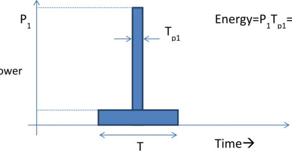
A signal gets attenuated while traversing through a channel. So for long range detection, the transmitted pulse should have high energy so that its echo from the target has sufficient energy to get detected at the receiver. Energy content of the transmitted pulse is given by the product of peak power and pulse duration of the pulse. Hence as shown in Figure 1-1, a high energy signal can be a pulse with high peak power and short pulse duration, or a longer duration

2 | P a g e

Figure 1-1 Pulses of different pulse duration but same energy

pulse of lesser pulse duration. Radar works at microwave frequencies, so transmitting a high peak power pulse is not practical, as it makes the radar equipmentcostlier and bulkier.So we are only left to use pulses with limited peak power and a longer pulse duration. A long duration pulse has got a very poor range resolution, this is why the technique of pulse compression must be used at the receiver.

1.1

Pulse Compression

With radar systems, longer pulses of limited peak power are to be used to ensure a large maximum range detection. But we must have a narrow signal with high peak power at the output of receiver in order to get a good range resolution. This problem is solved by pulse compression techniques which make it possible to avail the long range detection benefits of a long duration pulse without trading off the high range resolution benefits. In pulse compression, some modulation technique like frequency modulation or phase modulation is used to accommodate a larger bandwidth so as to get a higher range resolution. A long duration pulse of low peak power is frequency or phase modulated before transmission and the received signal is passed through a matched filter which accumulates the energy of signal to a narrow duration of time 1/B. The

P

Power

rr

Time



T

T

Energy=P

T

=

P

T

3 | P a g e

scale of compression relative to an uncompressed pulse is given by Pulse Compression Ratio

PCR

1.2

The compression ratio which gives a figure of merit for pulse compression is equal to the Time-Bandwidth product TB of the pulse.

1.2

Matched Filter

The pulse compression filter of a radar receiver is an implementation of matched filter [1]. The SNR of the received signal is of great importance in radar systems, because the probability of detecting the signal depends on the SNR rather than the exact shape of the signal. Hence it is more important to maximize the SNR rather than preserving the waveform of the signal. The output of a matched filter has the maximum signal to noise ratio (SNR) when the signal to which the filter is matched, plus the Additive White Gaussian Noise (AWGN) is passed through it. A matched filter is always a specific linear filter whose impulse response is a function of the specific signal to which that filter is matched. We can have a brief idea about the matched filter from the block diagram below in Figure1-2.

Figure1-2 Block diagram of matched filter

s(t) Matched Filter h(t), H(ω) s0(t)+n0(t) AWGN N0/2

4 | P a g e

The matched filter is fed with the signal s(t) and AWGN noise of power spectral density

N0/2. Now the aim is to find the impulse response h(t) or transfer function H(ω) that will cause a maximum output SNR at a predetermined delay t0. In short we need to maximize the function

( ) | _{̅̅̅̅̅̅̅̅̅̅̅} | 1.3

The impulse response of a matched filter is determined only by the specific waveform s(t) and the predetermined delay t0. If the Fourier transform of s(t) is S (ω), then the output signal at t0 is given by

∫ 1.4

The mean square value of noise which is independent of t is given by

̅̅̅̅̅̅̅̅ ∫ | | 1.5

Now substituting the values of (1.4) and (1.5) into (1.3) gives

(

)

∫ | | 1.6

Schwarz‟s inequality says that for any two complex signals A(ω) and B(ω), they saitisfy the following inequality :

|∫ | ∫ | | ∫ | | 1.7 Using Schwarz‟s inequality in (1.6) , it was found that

( ) ∫ | | 1.8

Where E is the energy of the finite time signal

5 | P a g e

It was found from Schwarz‟s inequality condition that the SNR is maximized only when

1.10

The above is thus the frequency response of the matched filter. The impulse response of the matched filter can be found out by just taking the inverse Fourier transform of (1.10)

1.11

It shows that the impulse response of a matched filter is a delayed complex conjugate of time inverse of the signal.

When the filter is matched to the transmitted signal, the output SNR at t=t0 for received signal corrupted with AWGN noise is the attainable maximum, which is SNR=2E/N0. It is to be observed that the maximum SNR is only a function of the energy of the signal and not the shape of the waveform. In essence, the matched filter results in a correlation of the received signal with the delayed version of transmitted signal.

1.3

Ambiguity Function

There may be two targets very close to each other while varying in their radial velocity. Therefor the radar receivers create filters matched not only to the transmitted signal but also to the various doppler shifted versions of it. Here it is now important to have a very narrow response in doppler too, so that two objects with different radial velocity can be uniquely identified. For the two targets case, each one will cause a peak at different doppler shifted matched filter. This requires the study of matched filter output in two different dimensions: delay (τ) and doppler (ν) . The ambiguity function (AF) represents the time response of a filter matched to a given finite energy signal when the signal is received with a delay τ and a doppler shift ν relative to the nominal values expected by the filter. Ambiguity function expression is given by

6 | P a g e

| | |∫ | 1.12

Where u is the complex envelope of the signal, τ is the delay and υ is the doppler shift. A positive delay τ means that the target is farther from radar with respect to reference τ=0. A positive υ means that the target is approaching towards the radar whereas a negative υ implies a receding target. Figure 1-3 shows the ambiguity function plot of the most basic signal, which is a

7 | P a g e

unmodulated pulse of duration T. The delay axis is normalized with T, whereas the doppler axis is normalized with 1/T.

1.3.1

Properties Of Ambiguity Function

The ambiguity function of signal satisfies the following properties :

1. The AF is maximum at its origin, where its energy is generally normalized to unity

| | | | 1.13

2. Irrespective of the type of signal, the total volume inside the normalized ambiguity surface is equal to unity.

∫ ∫ | | 1.14

3. The ambiguity plot of a signal is symmetric about its origin, hence it is sufficient to study the plot only in any two adjacent quadrants.

| | | | 1.15

4. If the complex enevelope of a signal u(t) has its AF= | |, then the quadratic phase modulation or linear frequency modulation of that pulse has the following effect:

| | 1.16

Then, | | 1.17

1.4

Radar Signals

A fixed frequency continuous wave signal of time duration T is not suitable due to its inability to resolve range for its narrow spectrum bandwidth B=1/T. Frequency and phase modulation techniques are generally used in order to broaden the spectrum of the signals, so that

8 | P a g e

they provide a higher range resolution. After the signals are modulated to contain a bandwidth B, the signals can then be pulse compressed using matched filter to a duration 1/B.

1.4.1

Phase Modulated Pulse

Figure 1-4 Binary phase coded pulse and its ACF

Phase coding is one of the earliest methods of pulse compression. A pulse of duration T is divided into M bits of identical duration tb=T/M, and each of the bits is coded with a different phase value. The complex envelope of a phase coded pulse is thus given as

√ ∑ *

₊

1.18

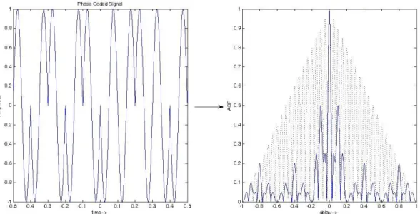
where um =exp(jπφm) and φm={φ1,φ2, φ3, φ4, … φM} represent the phase code for u(t). Although the possible number of phase codes that can be generated is large, the basic engineering task is to select the optimal codes for various applications. Resolution properties of the waveform, frequency spectrum, and the ease of implementation are the factors which play a key role to select a particular phase code. One can understand pulse compression by phase coding by simply considering binary phase shift keying technique. In this modulation scheme the code is made of

9 | P a g e

signal. Figure 1-4 shows the matched filter output of a binary phase coded pulse of 10 bits having the sequence [1 -1 1 -1 1 -1 -1 1 1 -1 ]. The dotted ACF plot corresponds to the unmodulated pulse and solid one is the ACF of phase coded pulse. It is observed that the ACF corresponding to phase coded pulse has a reduced width of mainlobe but suffers from sidelobes. Special cases of these binary codes are the Barker codes where the peak of the autocorrelation function is N (for a code of length N) and the magnitude of the maximum peak sidelobe is 1. The problem with the barker codes is that none with lengths greater than 13 have been found.

1.4.2

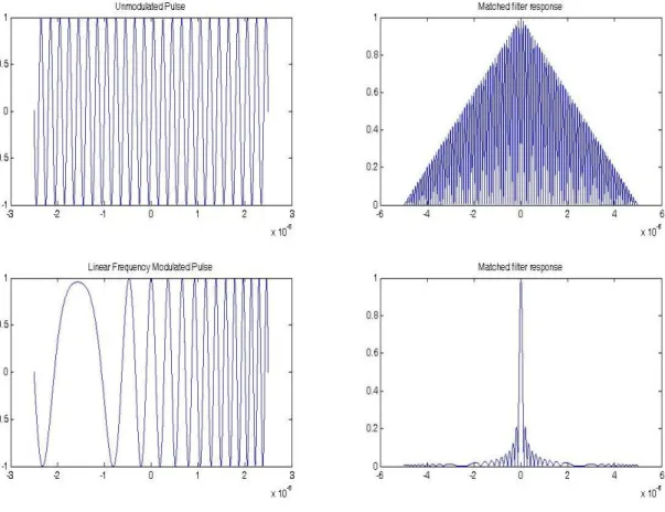
Frequency Modulated Pulse

The top-left plot of Figure 1-5 shows the unmodulated constant frequency pulse, and its ACF is shown on its right. It has a very poor range resolution due its narrow bandwidth. Frequency modulation is another alternative by which the spectrum of the transmitted pulse can be widened. Along this approach Linear Frequency Modulation (LFM) is a popular method, in which the instantaneous frequency of the pulse sweeps linearly through a predetermined bandwidth B during its pulse duration T .The complex envelope of an LFM pulse having unit energy can be expressed as

_√ ( )

where k is the frequency slope of the pulse, „+‟ denoting positive frequency slope and „−‟

denoting negative frequency slope. The instantaneous phase of the pulse is given by

1.20

The instantaneous frequency of the pulse can be found out by differentiating the phase with respect to time t.

10 | P a g e

Hence we find that the frequency of the pulse is a linear function of time and so it is called Linear Frequency Modulation.

Figure 1-5 Unmodulated pulse and its ACF, Bottom: LFM pulse of T=5 μs, B=8 MHz and its ACF

As can be observed from the bottom plot of Figure 1-5, the matched filter output of an LFM pulse definitely gives a high range resolution due to its narrow mainlobe but it also contains ambiguous sidelobes. These sidelobes can cause problems for the detection of weaker targets. The sidelobe having the highest magnitude in the ACF is called as the peak sidelobe. The lower the peak sidelobe, the better is a pulse compression technique which produced the respective ACF. Peak Sidelobe Ratio (PSR) is the term used to quantify the sidelobe performance of a pulse compression technique and is expressed as

11 | P a g e

PSR is a ratio and hence better expressed in dB. So in the same terms, we need to design pulse compression systems which has the lowest PSR performance.

1.4.3

Costas Frequency Coding

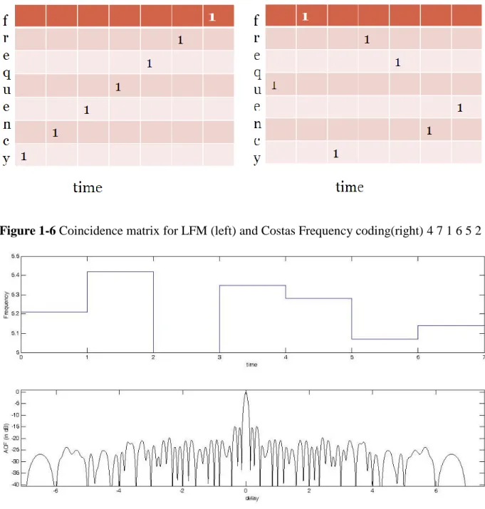
LFM Pulse discussed earlier is the most basic frequency modulated signal that can be used in radar systems. Another type of frequency modulation scheme called Costas Frequency Coding has a rather random-like frequency evolution. It was originally proposed by John P. Costas [2] as a discrete and non-linear frequency coding technique. It is quite opposite to that of LFM law and the difference can be well demonstrated by the binary matrix shown in Figure 1-6. The M contiguous time slices each of duration tb are represented by the colums and the rows represent the M distinct frequencies separated by a frequency ∆f. Both the matrices shown in the figure contain a single „1‟ in each row and each column. This is to show that only a unique frequency is transmitted at any time slice, each of the frequencies being used only once. Although there can be M ! possible ways of transmitting a frequency only once in a time slice, the frequency jump order affects the ambiguity function (AF) of the signal very strongly. For a rough prediction of the AF, one can overlay the matrix over itself and shift it to desired delay (horizontal shifts) and doppler (vertical shifts). If particular shifts in delay and doppler causes N

number of coincidences, then it is to be predicted that there will be a peak of N/M at that delay-doppler shift. In case of LFM, coincidence will result only for equal number of delay and delay-doppler shifts. Say for example, mtb delay and m∆f dopplershifts will result into N=M−m coincidences. Costas frequency jump sequence is unique in that, the number of coincidences can no more than one for any delay-doppler shifts except for zero shift case, when it has the maximum N=M

coincidences. This points to an ideal AF in which there is a narrow peak at the origin and there are very small sidelobes, AF getting better with increasing length of Costas sequence. Frequency

12 | P a g e

Figure 1-6 Coincidence matrix for LFM (left) and Costas Frequency coding(right) 4 7 1 6 5 2 3

Figure 1-7 Frequency evolution and ACF for Costas code sequence 4 7 1 6 5 2 3

evolution plot for a Costas sequence [4 7 1 6 5 2 3] and its ACF is shown in Figure 1-7. At an earlier stage many construction algorithms were given by Golomb and Taylor [3] but those algorithms work only for codes of certain small length only. So for longer length Costas codes, an exhaustive search into all possible frequency jump sequences of any dimension M must be made. A recent publications [4] - [5]enumerates Costas arrays of order 28, the enumeration been

13 | P a g e

performed on numerous computer clusters and required an equivalent of 70 years of single CPU time. So at present there are two domains of work related to Costas codes, one being the design of more efficient and faster algorithms to search down the Costas codes of higher orders, and secondly to use the existing arrays to design waveforms using various modified modulation schemes to get improved characteristics of AF. One such publication of later type is [6] which proposes to overlay a orthogonal set of N-phase codes on the modified costas pulses [7] for an improved performance.

Figure 1-8Ambiguity function of Stepped frequency train of unmodulated pulses, Tr/T=5

1.5

Conclusion

LFM pulse was the most basic frequency modulated pulse with its ambiguity function shown in Figure 1-3. It had a very poor range and doppler resolution, as was clear from the very

14 | P a g e

broad mainlobe, both in range and doppler axis. The linearly stepped frequency train of pulses has a better ambiguity function as shown in Figure 1-8. It has a narrower mainlobe width in

Figure 1-9Ambiguity function of Costas hopping sequence [4 7 1 6 5 2 3], Tr/T=5

delay due to its greater bandwidth content, while the lobes are still high. With the use Costas coding sequence with its ambiguity function shown in Figure 1-9, it gave a narrow mainlobe both in delay and doppler, and even very low sidelobes in both the axes. Again the height of the sidelobes with respect to the main lobe, or the PSR in Costas coding is inversely proportional to the length of the Costas sequence. The sidelobes were no more than 1/7thof the mainlobe height. Hence of all the unmodulated pulse waveforms discussed in this chapter, the ambiguity function of the Costas hopping sequence is most close to an ideal ambiguity function.

15 | P a g e

2

. Optimisation of Amplitude

Weighing Windows for

Sidelobe Reduction in LFM

Radar Pulse

16 | P a g e

FM pulses are used because it increases the bandwidth and thus the range resolution of the signal by a factor equal to time-bandwidth product TB. However for LFM pulse, the output of the matched filter suffers from very high range sidelobes as high as −13 dB. In radar applications, where there may be weak targets very close to a stronger target, the ACF sidelobes at the matched filter output due to echoes from the stronger target may mask the mainlobe of a weak targets. Moreover the sidelobes themselves may falsely be detected as weak targets. We know that fourier transform of ACF gives the power spectral density of a signal. Hence the ACF sidelobes can be reduced by shaping the spectrum. Spectral shaping can be done either by amplitude weighting or by frequency weighting [1]. Amplitude weighting is the approach taken here for shaping the spectrum of LFM pulses. Spectral shaping through amplitude weighting is based on the linear relation of the frequency with time in an LFM pulse. At any given instant of time, a particular frequency is transmitted. Therefore by shaping the amplitude of the pulse along time automatically shapes the power spectral density along frequency. Kaiser window [8] and Hamming window [9] have been used in the past for amplitude weighting in order to reduce the range sidelobes. In case of the Kaiser window appropriate β parameter had to be selected to control the sidelobe level and width of the main lobe. In this paper, new windows have been found out for minimum range sidelobe performance quantified by Peak Sidelobe Ratio (PSR). The temporal shaping-windows are expressed here as a finite sum of weighted cosines [10] over a time duration, and the weighting coefficients of the windows have been optimized by Clonal Particle Swarm Optimization [11] and Differential Evolution [12] to give minimal PSR.

17 | P a g e

2.1

Characterization of LFM chirp and weighting window:

The frequency of an LFM pulse evolve linearly in its pulse duration T to cover a bandwidth B. Its complex envelope can be expressed as

(

√ )

_{; 2.1}

and by differentiating the argument of the above exponential term gives the instantaneous frequency f(t) of the chirp

( ) 2.2

Figure 2-1 Frequency Evolution of LFM chirp T=8μs, B=10MHz

When LFM chirp is compressed by a matched filter at the receiver, we get range sidelobes occurring along with the main lobe which are often unacceptable. They can be countered by amplitude weighing the time domain signals. Amplitude weighing is implemented by various

18 | P a g e

pulse shaping window functions. This paper characterizes the window functions as a weighted sum of cosines [10]. These windows are completely characterised by the number of cosine terms and the coefficients used as the weight of cosines in the expression. The temporal weight windows used here are of the form:

∑ | | 2.3

where { } are real constants. Weighting is symmetric about t=0 and it is normalized according to :

∑ ∑ 2.4

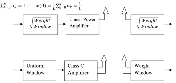
Figure 2-2 Matched weighting (top) and Mismatched weighting(bottom)

This is the general equation for realizing a temporal window, from which all the standard windows like Hanning window, Hamming window, Blackman window and others can be realised by assigning appropriate values to coefficients. The shaping is done in time domain, by multiplying the signal to be shaped with appropriate weight window. It can be done in either in the matched filtering way or in the mismatched filtering way. In matched filtering, weight is split between the transmitter and receiver i.e. the amplitude at each end is shaped by a square root of the window. The problem with this technique is that it requires a linear power amplifier causing inefficiency. Alternatively in mismatched filtering, the entire window is implemented at

√ Linear Power Amplifier √ Uniform Window Class C Amplifier Weight Window

19 | P a g e

the receiver end, having to compromise with resulting loss in Signal to Noise Ratio (SNR) due to mismatched filtering.

2.2

Clonal Particle Swarm Optimization (CPSO) :

Particle Swarm Optimisation (PSO) [13] is basically a stochastic optimization technique inspired by the coordinated and collective behavior of birds in a flock. The search space is an n-dimensional space where the n dimensions comprise of those independent variables on which the solution of the problem depends. A bunch of candidate solutions termed as particles are randomly initialized in the search space and are let to explore for the best solution of the problem. These randomly initialised particles in the search space are collectively called as a swarm. Each particle updates both its position and velocity iteratively according to its personal best position found so far, and the current best position out of all the particles achieved as yet. The particles search for the optimal solution by iteratively evolving themselves while their fitness value is evaluated at every evolution by the fitness function. As according to the Standard Particle Swarm Optimization (SPSO), given by James Kennedy and Russell Eberhart [13], the update formula for velocity and position is given by the following equations:

( ) ( ) 2.5

2.6

where i=1, 2,…, n is the particle count in the swarm and, d=1, 2,3,…, D is the dimension of the solution space. is the ith particle‟s best d-dimension as achieved yet, whereas is the

achieved d-dimension of the global best particle in the swarm. Constants c1, c2 are non-negative learning factors, and r1, r2 are the random numbers from a uniform distribution [0 1]. The parameter w Є [0 1] is the inertia weight factor, w being large is appropriate for global search whereas a small w is good for local search.

20 | P a g e

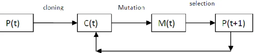
Standard Particle Swarm Optimisation guides the swarm to converge to a single optima with the help of particles having the best known positions in the search space. But in the problems where there are multiple optima, choosing the best fit particle to guide the swarm is a critical issue. A wrong choice of best-fit particle may mislead the swarm to a local optimum and get stuck there. Here is when the Clonal Particle Swarm Optimization (CPSO) [14] comes to rescue and guides the SPSO to escape from local minima while searching for the global optima efficiently. The introduction of clonal expansion process in SPSO strengthens the interaction between the particles in the swarm and enhances global convergence performance. Global best particle of each SPSO generation is kept in memory to act as mother particles. A new step called cloning operation is allowed where a mother particle is cloned up to N identical particles in the search space, which are then used to generate N new particles through clonal mutation. During the mutation stage, random variations are done around each of the N similar cloned particles. This is like making a deliberate more extensive search around the most promising particles through generations. It accelerates the evolution process for better optimization and a faster convergence.

2.2.1

PSO Algorithm To Find Specific Window Coefficients For

Optimal PSR

Here, the CPSO technique has been used to find windows for specific time-bandwidth products TB, which can result in amplitude weighing of the LFM pulse to give the least PSR at the matched filter output. The K coefficients of the cosine-based window expression given by (2.3) vary along the corresponding K axes of the search space. The coefficients take values in the search space only after satistfying the constraints provided for the them in (2.4). Hence each of the particles in the swarm represent a window used for amplitude weighing of pulse. The

21 | P a g e

particles in the swarm are to search for the position causing the minimal PSR. The step trasition in a CPSO algorithm can be represented as follows:

Figure 2-3 State transition for CPSO

Step 1 Initialization: The initial number of swarm particles are initialized. To start with, the particles are randomly positioned in the search space against the K dimensions, essentialy satisfying the constraints defined in (2.4).

Step 2 Pulse shaping and compression: The defined LFM pulse of duration T and bandwidth B is shaped by the windows as represented by the particles in the swarm and is compressed as per requirement, by either matched filtering or mismatched filtering. The corresponding ACF, and hence PSR is a function of position of the particles, i.e. the window coefficients. PSR corresponding to each of the particles acts as the fitness function for this optimization problem.

Step 3 SPSO stage: The particles are let to update their position and velocity according to (2.5) and (2.6) iteratively for M number of generations. Particle with a set of window coefficients causing a lower PSR competes ahead to decide for particle‟s personal best and the spot for global best particle in the swarm.

Step 4: The global best particle at the end of each generation is stored in memory as mother-particles for use in the subsequent cloning phase.

22 | P a g e

Step 5: After the completion of M SPSO generations, the window coefficients corresponding to the last registered global best particle and its resulting sidelobe level is recorded out separately.

Step 6 Cloning: The particles in memory as mother-particles which acted as a global best particle for at least one generation are cloned into several particles.

Step 7 Mutations: Each of the cloned particles is mutated in all dimensions by some random disturbance, Gaussian noise in this case of zero mean and unity variance. Mutation can hence be represented as:

2.7

Where s is the scale of mutation and Vmax is the maximum velocity of mutation.

Table 1 PSO optimised window coefficients at specific time-bandwidth for minimum PSR; left: three coefficient window; right: four coefficient window

PSO Filter a0 a1 a2 PSR TB a0 a1 a2 a3 PSR MMF 0.5067 0.4877 0.0056 -28.7481 20 0.5047 0.4632 0.0122 0.0199 -29.1383 MF 0.3961 0.4996 0.1043 -54.9359 20 0.3459 0.4836 0.1542 0.0163 -62.5264 MMF 0.5074 0.4786 0.0140 -34.6375 40 0.4983 0.4869 0.0054 0.0094 -34.9262 MF 0.4005 0.4994 0.1001 -57.0215 40 0.3433 0.4821 0.1567 0.0179 -69.6731 MMF 0.5080 0.4808 0.0112 -38.2162 60 0.4905 0.4874 0.0161 0.0060 -38.2852 MF 0.4059 0.4999 0.0942 -60.7442 60 0.3478 0.4851 0.1522 0.0149 -78.5579 MMF 0.4935 0.4868 0.0197 -40.664 80 0.4988 0.4803 0.0151 0.0058 -40.7781 MF 0.4139 0.4993 0.0868 -62.1501 80 0.3610 0.4900 0.1390 0.0100 -78.0703 MMF 0.4859 0.4891 0.0250 -42.5462 100 0.4740 0.4941 0.0314 0.0032 -42.5492 MF 0.4111 0.4994 0.0895 -64.5113 100 0.3611 0.4897 0.1389 0.0103 -80.1701

23 | P a g e

Step 8: Now these mutated particles form the particles of a new swarm which undergoes step-2 to step-8 for some S-1 number of cycles.

Step 9 Termination: Step 8 continues for S-1 cycles, and the algorithm stops at the Sth cycle‟s step-5. Out of all the results accumulated in step 5 during the cycles, the window coefficients corresponding to lowest PSR is recorded for the optimal window parameters.

2.3

Differential Evolution (DE) :

Differential Evolution [15] is a search and optimization method which came as a result of the keen observation of the researchers into the underlying relation between optimization and the biological evolution process. Direct search methods are chosen whenever the cost function to be minimized is of non-linear and non-differentiable nature. DE is a powerful direct search stochastic optimization algorithm. In this a fitness function or objective function is designed to measure the extent of performance in the optimization problem. The aim is to find out a set of parameters which makes the system to perform at its best under certain conditions. The set of parameters governing the fitness function and hence performance of the system is represented by a parameter vector. Like any other direct search method the central strategy of DE is to generate variation of the parameter vectors and then to put them under check if or not to accept the new parameters. If the new parameter vector gives a lower value of the fitness function than its parent parameter vector, it replaces the parent parameter vector. Parallelizability of DE helps it to cope up with computation intensive fitness functions and also safeguards it from converging to a local minimum. Several vectors run simultaneously, therefore a better performing parameter vector can rescue the algorithm form being trapped into a local minimum. DE is an easy to use algorithm using a few control variables to steer the minimization procedure. It is also self-organizing in nature using the existing vectors to find differences between them to create new

24 | P a g e

parameter vectors with the help of control variables. DE replaces an existing vector with a new one in the next generation, if it performs better for the fitness function.

2.3.1

DE Algorithm To Find Specific Window Coefficients For

Optimal PSR

DE algorithm searches a D-dimensional parameter space for the global minimum. For the present problem D-dimensions are the variations in K coefficients in cosine based window expression given in (2.3). The fitness function to minimize here is the PSR at the matched filter output, that amplitude weighing of the LFM pulse by a particular window can attain. Optimization of this problem through DE works through iterative stage cycles as shown in the Figure 2-4:

Figure 2-4 Stages of Differential Evolution

Step 1 Initialization of parameter vectors: A population of NP≥4 number of D-dimensional parameter vectors is randomly initiated to cover the parameter space uniformly. Each parameter vector represents a cosine based window function that acts as a candidate solution for the PSR minimization problem, so we will term it as a window vector. The ith window vector of the population is represented as:

2.8

where G is the generation number. Initialization

of vectors

25 | P a g e

Step 2 Mutation: Mutant window vector is generated by taking each vector of the population as a target vector . A weighted difference of two population vectors is added to a third one to get the mutant vector.

( ) 2.9

The indices i, r1, r2, r3 Є {1, 2, 3,…, NP } are mutually different and F>0. FЄ [0 2] controls the amplification of the difference vector.

Step 3 Crossover: The mutant vector is then mixed with the target vector to get the trial vector according to the law:

{

} 2.10

j=1, 2, 3,…D

In the above equation rand(j) is the jth uniform random number evaluation, CR is crossover constant Є [0 1] determined by the user and randbr(i) is a randomly chosen index from 1,2,3,…,D.

Step 4 Selection: If the trial vector produces a lower PSR value than the target vector, it replaces the target vector in further generations. This operation is called as selection. Each population vector must once act as a target vector so that there are NP competitions, each vector getting its chance to evolve through mutation, crossover and selection in a generation.

Step 5 Termination: Each of the NP vectors getting a chance as trial vector, and each reaching the selection stage once, completes a single generation of DE. After the completion of a generation, the next generation puts the algorithm back to the mutation stage. Meanwhile a record-keeper function keeps updating itself with the window vectors with better fitness function

26 | P a g e

value generation after generation and trial after trial. Termination is made after a sufficiently large number of generations wave passed such that the PSR saturates around some minimum value recorded by the record-keeper function.

2.4

Results and discussion:

It is very difficult to obtain low sidelobes for time-bandwidth product TB less than 100 due to the amplitude ripple of LFM chirp signal. It was found by Milewski, Sedek, Gawor [9] that smaller the TB, larger the amplitude ripple becomes and the greater there is sidelobe degradation.

Table 2 DE optimised window coefficients at specific time-bandwidth for minimum PSR; left: three coefficient window; right: four coefficient window

DE Filter a0 a1 a2 PSR TB a0 a1 a2 a3 PSR MMF 0.4985 0.4958 0.0057 -28.7640 20 0.5047 0.4632 0.0122 0.0199 -29.1383 MF 0.3963 0.4996 0.1041 -54.9130 20 0.3472 0.4845 0.1528 0.0155 -63.2136 MMF 0.5062 0.4849 0.0089 -34.7105 40 0.5006 0.4814 0.0075 0.0105 -34.9000 MF 0.4042 0.4996 0.0962 -60.3298 40 0.3520 0.4865 0.1480 0.0135 -70.1264 MMF 0.4906 0.4904 0.0190 -38.1974 60 0.5043 0.4795 0.0099 0.0063 -38.3357 MF 0.4075 0.4996 0.0929 -62.4224 60 0.3480 0.4843 0.1520 0.0157 -75.6938 MMF 0.4961 0.4856 0.0183 -40.6640 80 0.5130 0.4665 0.0156 0.0049 -40.6590 MF 0.4094 0.4995 0.0911 -63.7180 80 0.3387 0.4814 0.1613 0.0186 -79.0505 MMF 0.5120 0.4752 0.0128 -42.5719 100 0.4913 0.4836 0.0206 0.0045 -42.6343 MF 0.4111 0.4994 0.0895 -64.5113 100 0.3434 0.4834 0.1566 0.0166 -84.6514

CPSO algorithm and DE as described above were used to find out minimal PSR producing windows of the form (2.3) for typical TB values. Optimal windows giving a minimum PSR performance were obtained both for matched filtering and mismatched filtering modes. Table 1

27 | P a g e

presents the Clonal PSO-optimized matched filter and mismatched filter PSR, along with respective window coefficients. Window coefficients were obtained for both three coefficient window and four coefficient windows. Table 2 presents results obtained through DE optimization with the same objective as was for Table 1.

Comparison with other standard windows: Table 3 shows the sidelobe reduction performance of some standard windows namely Hamming window, Hanning window and Kaiser window along with the new windows those were obtained after optimization through CPSO and DE. It is observed in the mismatched filtering case, that some conventional windows perform closely as good as those found out by clonal PSO and DE. While Hamming windows are inconsistently close to the optimum sidelobe level of mismatched filtering, Kaiser window reduces the sidelobes close around optimum quite consistently. So for the mismatched filtering case, it is fair enough to generalize that the Kaiser window with β=6 provides the best sidelobe reduction avoiding any requirement of sidelobe reduction through optimization techniques. When there is an option to choose from matched filtering and mismatched filtering, the latter one definitely does remarkably well in sidelobe reduction for any chosen window. By the use of matched filtering, it also avoids SNR loss due to mismatch. Of all the conventional windows taken, the Kaiser window with β=6 gives the minimum sidelobe. For matched filtering, the CPSO and DE windows do exceptionally well to reduce the sidelobe levels as compared to the conventional windows. Taking for example the second case of Table 3 where time-bandwidth product is 40, the Kaiser window gives a sidelobe level of -41.2929 dB, whereas optimization results through DE for four coefficients gives a reduction up to -70.1264 dB as depicted in Figure 2-5. It is clear from Table 3 that, it is fair enough to generalize that the CPSO

28 | P a g e

Figure 2-5 Sidelobe comparision of Kaiser window and 4-coeff-DE-window, TB=40 and DE windows for matched filtering are the best option, when sidelobe reduction is the foremost priority.

Effect of increasing window coefficients: Windows of the form (2.3) can be well-designed with k>=2. The greater the number of ak coefficients, the more precise spectral shaping is possible. In case of mismatched filtering, there is hardly any improvement in the sidelobe reduction in moving from three-coefficients to four coefficients. At the same time, in matched filtering, we can see a noticeable reduction in the PSR in moving from three coefficients to four coefficients.

29 | P a g e

As shown in Figure 2-6, when we move from three coefficient DE optimized window to four coefficient DE optimized window for TB=100, the PSR goes down remarkably from −64.5113 dB to −84.6514 dB. So it shows that increasing the window coefficients improves the pulse shaping of the LFM pulse for a better sidelobe minimization.

30 | P a g e

Table 3 Comparative PSR levels of classical windows versus CPSO and DE optimised windows

TBW Filter Hamming Hanning Kaiser _(β=6) PSO (3coef) PSO (4coef) DE (3coef) DE (4coef) 20 MMF -28.5377 -28.6761 -28.7271 -28.7481 -29.1383 -28.7640 -29.1383 20 MF -33.5784 -29.8352 -37.4059 -54.9359 -62.5264 -54.9130 -63.2136 40 MMF -34.5555 -31.0930 -34.8108 -34.6375 -34.9262 -34.7105 -34.9000 40 MF -37.7184 -30.9123 -41.2929 -57.0215 -69.6731 -60.3298 -70.1264 60 MMF -38.0559 -31.3692 -38.3879 -38.2162 -38.2852 -38.1974 -38.3357 60 MF -39.7027 -31.1989 -42.4288 -60.7442 -78.5579 -62.4224 -75.6938 80 MMF -39.8446 -31.4298 -40.8536 -40.664 -40.7781 -40.6640 -40.6590 80 MF -40.6627 -31.3114 -42.9069 -62.1501 -78.0703 -63.7180 -79.0505 100 MMF -40.6143 -31.4495 -42.7749 -42.5462 -42.5492 -42.5719 -42.6343 100 MF -41.2127 -31.3658 -43.1547 -64.5113 -80.1701 -64.5113 -84.6514

2.5

Conclusion:

Shaping of the signals by weighting windows has been one of the ways to reduce the range sidelobes in LFM signals. CPSO and DE technique have been used to find out those optimum windows for signals of specific time-bandwidth products in both matched and mismatched filtering modes. Sidelobe degradation is worst for TB less than 100, especially where the matched filter with optimized windows can come to a great rescue to suppress the sidelobes. In addition to the advantage of no SNR loss due to mismatch in the matched filtering, the CPSO and DE optimized windows reduce the PSR far below the levels that could be achieved by conventional windows. The only trade off being the broadening of the main lobe which degrades the vertical resolution of the radar signal.

31 | P a g e

3

. Stepped Frequency Train

32 | P a g e

idening the spectrum of the transmitted radar pulse is necessary for an enhanced range resolution. A step ahead in this direction is to use a train of pulses with Tr being the pulse repetition time, with a frequency step ∆f between consecutive pulses [16]. It also has an advantage of providing a large total bandwidth while the instantaneous bandwidth is quite narrow. The duration between the pulses can be used by the radar components to prepare for the narrow band frequency step of the next pulse. A large

∆f between pulses ensures a larger total bandwidth. But when the product of frequency step ∆f and pulse duration T becomes greater than 1 (T∆f>1), the autocorrelation function ACF of the stepped frequency train of pulses suffers from ambiguous peaks which are called as grating lobes [16]. It has been observed that using Linear Frequency Modulated LFM instead of fixed frequency pulses in the train of pulses, with their centre frequencies stepped by ∆f has an effect of reducing the grating lobes. This phenomena has been exemplified by the plots in Figure 3-1and Figure 3-2, which shows that the use of LFM pulses has a reducing effect on the grating lobes. ACF of a single LFM pulse has sidelobes and nulls, whereas a train of pulses causes grating lobes due to the frequency steps. From the Ambiguity Function AF expression of the train of pulses, a relationship between T, B and ∆f can be derived to place the nulls of LFM-ACF exactly at the position of grating lobes, hence nullifying the grating lobes.

3.1

Ambiguity Function For Stepped Frequency Train Of LFM

Pulses

The complex envelope of a single LFM pulse having unit energy is given by u(t)in (1.18). Applying (1.18) to the general eqation for AF of a signal given in (1.11), the AF of a single LFM pulse can be expressed as

| | |( | |) * ( | |)+| 3.1 For our requirement we have a train of N such LFM pulses with a pulse repetition time Tr>2T.

33 | P a g e

Figure 3-1 Amplitude (top), frequency evolution (middle) and ACF(bottom) of stepped frequency train of six pulses

34 | P a g e

Figure 3-2 Amplitude (top), frequency evolution (middle) and ACF(bottom) of stepped frequency train of six pulses

35 | P a g e

√ ∑

3.2

Unit energy is maintained by dividing by the expression √ . For delay τ less than pulse duration

T, the ambiguity function of a train of pulses is related to the ambiguity function of a single pulse according to

| | | | | | ; τ≤T 3.3

Now adding LFM to the train of pulses for frequency stepping through a new slope ks, gives the expression for stepped frequency train of LFM pulses.

= _√ ∑ 3.4 where , ∆f > 0

„+‟ sign representing a positive frequency step and „−‟ sign representing a negative frequency step. Putting LFM frequency step modifies the ambiguity function of the signal as

| | | | 3.5

Putting (3.3) in (3.5) we get

| | | | | | 3.6 Combining (3.1) and (3.6), we get the ambiguity function of stepped frequency train of LFM pulses

| | |( | |) * ( | |)+| | |; |τ| ≤T 3.7

Hence we find that the slope ks for frequency step adds up to the slope of LFM chirp in a single pulse, so the ultimate bandwidth of the signal becomes

3.8

Ambiguity function expression in (3.7) can be further simplified to

| | |( | |) * ( ) ( | |)+| |

( ( ) )

36 | P a g e

3.2

Nullifying Grating Lobes

The ACF of stepped frequency train of LFM pulses can be obtained by putting ν=0 in (3.9) producing

| | |( | |) * ( | |)+| | | ; |τ| ≤T 3.10

Figure 3-3 Tr/T=2, TB=0, T∆f=5, Top: R1(τ) in solid, R2(τ) in dashed ; Bottom: ACF The expression in equation (3.10) is made up of two terms

| | |( | |) * ( | |)+| 3.11

37 | P a g e

The first term|R1(τ)| is due to a single LFM pulse of increasing slope, whereas the second term

|R2(τ)| represents the grating lobes [17] that is due to the frequency stepping of the consecutive pulses. |R2(τ)| exhibits its peaks (mainlobe and sidelobes ) at

, g= 0, ±1, ±2, ±3,…└T∆f┘ 3.13

Figure 3-4 Tr/T=2, TB=12.5, T∆f=5, Top: R1(τ) in solid, R2(τ) in dashed; Bottom: ACF Nullifying the grating lobes requires placing the grating lobes of R2(τ) exactly at the nulls of

R1(τ). The approach for this involves making the coincidence of first two grating lobes with the nulls of R1(τ). In some cases the fulfillment of this requirement nullifies all the grating lobes. For example, requiring that R1(τ) will exhibit it‟s 2nd and 3rd nulls exactly at the first two gratings lobes, namely at T=1/∆f and T=2/∆f respectively, yields the following two relationships: T∆f=5

and TB=12.5. The resulting nullification of grating lobes can be seen by comparing the plots in Figure 3-3 and Figure 3-4. The five grating lobes corresponding to T∆f=5 present with the use of fixed frequency pulses can be prominently seen in the Figure 3-3. The plots in Figure 3-4

38 | P a g e

shows that the use of LFM pulses with appropriate T∆f and TB values results in nulls exactly at the positions where the grating lobe peaks were present. So the final ACF function (Figure 3-4 bottom) is completely free from all the grating lobes.

3.3

T∆f

-

TB

Conditions For Grating-Lobe Nullification

Conditions for nullification of grating lobes can be found out by deriving the condition in which the mth and nth nulls of R1(τ) fall at the qth and rth grating lobes at τ=q/∆f and τ=r/∆f . Applying this to (2.11) gives the following two relations :

( ) 3.14

( ) 3.15

The requirement of nullifying the first two grating lobes ,namely for q=1, r=1 and solving for

T∆f and TB yields

3.16

3.17

3.4

Conclusion

A good range resolution required a wide bandwidth, which we see that can be attained easily by stepped frequency train of pulses. Even the grating lobes can be nullified with the use of LFM pulses with proper choice of TB and T∆f from (3.16) and (3.17). This scheme originally described in publication [16] had a overall bandwidth of B+(N−1)∆f . The bandwidth can be increased further by making Tr=T, which will basically increase the number of pulses in the train by making the pulses contiguous. The next chapter discusses the problem arising from using contiguous pulses, and a new scheme has been proposed to solve the problem.

39 | P a g e

4

. Stepped-Frequency Train

40 | P a g e

ullification of the grating lobes with the scheme described in the previous chapter is valid if and only if Tr/T>2. It restricts the extent of increase of bandwidth by limiting the number of frequency steps for a signal of particular time. Here in this chapter ,a new scheme has been proposed that allows to accommodate more bandwidth by taking Tr/T=1, which means that contiguous pulses make up the pulse train .By this way, the number of frequency stepping can be made maximum for the same interval of signal, hence can accommodate more bandwidth. This will further increase the range resolution of the signal. But while doing the same, some of the grating lobes that were nullified with the use of LFM with suitable T∆f, TB pair are no more identically zero.

4.1

Effect Of Contiguously Aligned Pulses On The ACF

Figure 4-1 Alignment of received pulses with reference pulses to show ACF contribution Converting the train of separated pulses into contiguous subpulses (Tr = T) changes the ACF. Let the complex envelope of the different pulses be represented by up(t) ,where p denotes the pulse number. Then the ACF of the train of pulses in the delay region |τ|<T can be expressed as

∑ ∑ 4.1

41 | P a g e

So the ACF of the signal consists of the correlation terms of the delayed pulse with its corresponding reference pulse, and crosscorrelation terms of the delayed pulse with the adjacent reference pulse. This can be explained from Figure 4-1 in which reference pulse u2 has correlation with a part of identical delayed pulse u2 and cross-correlation with u1. The first sum of (4.1) is the dominant term in the ACF which is exactly the same when the pulses were separated and is expressed by (3.10). This first sum may exhibit grating lobes for fixed frequency pulses or may be nullified with the use of proper LFM. It does not depend on the slope polarity of the individual LFM pulses. The changes in the ACF over |τ|<T (where the grating lobes are found) are due to the second sum of (4.1) which is due to the cross correlation between adjacent pulses. The second sum does depend on the LFM slope polarity of the individual pulses. At higher delays of τ<T, only the cross terms are found in the ACF. The cross terms involving adjacent pulses, with slope polarity of LFM pulses remaining same has been found to be | | | * (( ) ) + (( ) ) | ;0 ≤τ ≤ T 4.2

Here, kp is an interger so that kp∆f denotes carrier frequency of the pth pulse. So in order to check if the nullifying holds we should be interested in the value of cross correlation terms(4.2) at the position of the grating lobes, namely at τ = g/∆f where g is an integer smaller than T∆f.

| ( )| | *

( )+

(( ) )

| ; 0 ≤τ ≤ T 4.3

The numerator of (4.3) is zero only when the argument of sine function is an intergral multiple of π. Substituting the T∆f and TB values from (3.16) and (3.17) gives the argument of the sine after dividing by π as , which is always an integer for r(r-1) is always even. The

42 | P a g e

The only time when cross terms do not become zero is when the denominator also becomes zero making it into a form. For this case of situation we loose the nullification at the point of

grating lobes, which was earlier done by a suitable pair of T∆f and TB values. It does not mean that the grating lobe is restored at the point. It only implies that the ACF at the point is no more identically zero and may be objectionable at times.

Table 4 Location of peak sidelobe on delay axis for various T∆f and TB Tp∆f TpB B/∆f Sidelobe position on delay axis (τ/Tb) dB 2 4 2 1.507 -9.4432 3 4.5 1.5 0.67 -5.0786 3 9 3 1.667 -7.0396 5 12.5 2.5 0.8 -3.5156 3 13.5 4.5 2.667 -9.5420 4 16 4 1.751 -6.0146 3 18 6 3.667 -13.0538

Table 4 shows the various T∆f & TB pairs with their respective highest recorded sidelobe level and its position on delay axis. We can see that the cancellation of grating lobes has failed for two of the cases namely, case-I: T∆f=5 & TB=12.5 and case II: T∆f =3 & TB=4.5 when Tr/T=1 was implemented. In these two of the cases, a significant lobe is observed within the delay τ<T, due to the above mentioned reason of failure in cancellation of grating lobes. Figure 4-2 shows the frequency evolution and corresponding ACF of stepped frequency train of six contiguous LFM pulses with T∆f =3 & TB=4.5, which is one of cases of failure in nullification of grating lobe mentioned above. We observe a prominent lobe which is as high as -5.0786 dB at the position of

43 | P a g e

the second grating lobe, which failed to be nullified after we made the pulses contiguous. Since this high lobe is within a delay less than the pulse duration, it may mask other targets or itself falsely act a target. It is undesirable and needs to be suppressed by some means.

Figure 4-2 Frequency evolution and ACF of contiguous constant slope LFM pulses Tr/T=1,

T∆f =3 & TB=4.5

4.2

Proposed Solution

Since the high ACF lobe at the position of grating lobes is grossly due to the cross-correlation between adjacent pulses, it can be reduced if the adjacent pulses in the stepped frequency train of pulses are spectraly isolated by some extent. One way of doing the same can be the use alternating LFM slopes for the contiguous pulses as the adjacent pulses do have some extent of overlap in bandwidth parameterized by the B/∆f ratio. The effect of B/∆f ratio on the grating lobes of stepped frequency pulses has been well described in publication [18]. The spectral overlap between the adjacent frequencies is maximum and by alternating the slopes of adjacent pulses the frequency isolation between them is increased. In contrast to the plots of Figure 4-2, the plots in Figure 4-3 shows the frequency evolution of stepped-frequency train of

44 | P a g e

Figure 4-3 Frequency evolution and ACF of contiguous alternating slope LFM pulses Tr/T=1,

T∆f =3 & TB=4.5

alternating slope LFM pulses with its corresponding ACF. It clearly shows the reduced lobe level at the position of second grating lobe which is now around -20 dB. So it is now possible to transmit contiguous train of pulses without loss of grating lobes nullification. It has a added benefit to the maximum range of detection of the radar waveform. Since for the same signal time it is now possible to accommodate more number of pulses, so the total energy content of the waveform also increases. A waveform having more energy can travel more distance hence increasing the maximum range of the radar system.

4.3

Conclusion

Maintaining one of the several possible relationships between the frequencyspacing ∆f, pulse duration T and the LFM bandwidth B, along with the use of alternate slope polarity for adjacent frequencies can reduce the high ACF lobes at the positions of grating lobes in the stepped frequency train of contiguous pulses. Distribution of ACF lobes become more uniform to ultimately reduce the spikes. This makes possible for the use of Tr/T=1, which ultimately