Weighted False Discovery Rate Control in Large-Scale Multiple Testing

University of Pennsylvania

ScholarlyCommons

Statistics Papers

Wharton Faculty Research

6-26-2017

Weighted False Discovery Rate Control in

Large-Scale Multiple Testing

Pallavi Basu

University of Southern California

Tony Cai

University of Pennsylvania

Kiranmoy Das

Indian Statistical Institute

Wenguang Sun

University of Southern California

Follow this and additional works at:

https://repository.upenn.edu/statistics_papers

Part of the

Business Commons

, and the

Statistics and Probability Commons

This paper is posted at ScholarlyCommons.https://repository.upenn.edu/statistics_papers/2 For more information, please [email protected].

Recommended Citation

Basu, P., Cai, T., Das, K., & Sun, W. (2017). Weighted False Discovery Rate Control in Large-Scale Multiple Testing.Journal of the American Statistical Association,http://dx.doi.org/10.1080/01621459.2017.1336443

Weighted False Discovery Rate Control in Large-Scale Multiple Testing

Abstract

The use of weights provides an effective strategy to incorporate prior domain knowledge in large-scale inference. This paper studies weighted multiple testing in a decisiontheoretic framework. We develop oracle and data-driven procedures that aim to maximize the expected number of true positives subject to a constraint on the weighted false discovery rate. The asymptotic validity and optimality of the proposed methods are established. The results demonstrate that incorporating informative domain knowledge enhances the interpretability of results and precision of inference. Simulation studies show that the proposed method controls the error rate at the nominal level, and the gain in power over existing methods is substantial in many settings. An application to genome-wide association study is discussed.

Keywords

Class weights, Decision weights, Multiple testing with groups, Prioritized subsets, Value to cost ratio, Weighted p-value

Disciplines

Weighted False Discovery Rate Control in Large-Scale

Multiple Testing

Pallavi Basu1_{, T. Tony Cai}2_{, Kiranmoy Das}3_{, and Wenguang Sun}1

August 5, 2015

Abstract

The use of weights provides an effective strategy to incorporate prior domain

knowl-edge in large-scale inference. This paper studies weighted multiple testing in a

decision-theoretic framework. We develop oracle and data-driven procedures that aim to

maxi-mize the expected number of true positives subject to a constraint on the weighted false

discovery rate. The asymptotic validity and optimality of the proposed methods are

established. The results demonstrate that incorporating informative domain knowledge

enhances the interpretability of results and precision of inference. Simulation studies

show that the proposed method controls the error rate at the nominal level, and the

gain in power over existing methods is substantial in many settings. An application to

genome-wide association study is discussed.

Keywords: Class weights; Decision weights; Multiple testing with groups; Prioritized

subsets; Value to cost ratio; Weightedp-value.

1_{Department of Data Sciences and Operations, University of Southern California. The research of}

Wen-guang Sun was supported in part by NSF grant DMS-CAREER 1255406.

2_{Department of Statistics, The Wharton School, University of Pennsylvania. The research of Tony Cai}

was supported in part by NSF Grants DMS-1208982 and DMS-1403708, and NIH Grant R01 CA127334.

3

1

Introduction

In large-scale studies, relevant domain knowledge, such as external covariates, scientific insights and prior data, is often available alongside the primary data set. Exploiting such information in an efficient manner promises to enhance both the interpretability of scientific results and precision of statistical inference. In multiple testing, the hypotheses being investigated often become “unequal” in light of external information, which may be reflected by differential attitudes towards the relative importance of testing units or the severity of decision errors. The use of weights provides an effective strategy to incorporate informative domain knowledge in large-scale testing problems.

In the literature, various weighting methods have been advocated for a range of multiple comparison problems. A popular scheme, referred to as thedecision weights or loss weights approach, involves modifying the error criteria or power functions in the decision process (Benjamini and Hochberg, 1997). The idea is to employ two sets of positive constants

a

aa = {ai : i = 1,· · ·, m} and bbb = {bi : i = 1,· · · , m} to take into account the costs

and gains of multiple decisions. Typically, the choice of the weightsaaa and bbb reflects the degree of confidence one has toward prior beliefs and external information. It may also be pertinent to the degree of preference that one has toward the consequence of one class of erroneous/correct decisions over another class based on various economical and ethical considerations. For example, in the spatial cluster analysis considered by Benjamini and Heller (2007), the weighted false discovery rate was used to reflect that a false positive cluster with larger size would account for a larger error. Another example arises from genome-wide association studies (GWAS), where prior data or genomic knowledge, such as prioritized subsets (Lin and Lee, 2012), allele frequencies (Lin et al., 2014) and expression quantitative trait loci information (Li et al., 2013), can often help to assess the scientific plausibility of significant associations. To incorporate such information in the analysis, a useful strategy is to up-weight the gains for the discoveries in preselected genomic regions

by modifying the power functions in respective testing units (P˜ena et al., 2011; Sun et al., 2015). We assume in this paper that the weights have been pre-specified by the investigator. This is a reasonable assumption in many practical settings. For example, weights may be assigned according to economical considerations (Westfall and Young, 1993), external covariates (Benjamini and Heller, 2007; Sun et al., 2015) and biological insights from prior studies (Xing et al., 2010).

We mention two alternative formulations for weighted multiple testing. One popular method, referred to as theprocedural weights approach by Benjamini and Hochberg (1997), involves the adjustment of thep-values from individual tests. In GWAS, Roeder et al. (2006) and Roeder and Wasserman (2009) proposed to utilize linkage signals to up-weight the p -values in preselected regions and down-weight the p-values in other regions. It was shown that the power to detect association can be greatly enhanced if the linkage signals are infor-mative, yet the loss in power is small when the linkage signals are uninformative. Another useful weighting scheme, referred to as theclass weights approach, involves allocating var-ied test levels to different classes of hypotheses. For example, in analysis of the growth curve data (Box, 1950), Westfall and Young (1993, page 186) proposed to allocate a higher family-wise error rate (FWER) to the class of hypotheses related to the primary variable “gain” and a lower FWER to the secondary variable “shape”.

We focus on the decision weights approach in the present paper. This weighting scheme is not only practically useful for a wide range of applications, but also provides a powerful framework that enables a unified investigation of various weighting methods. Specifically, the proposal in Benjamini and Hochberg (1997) involves the modification of both the error rate and power function. The formulation is closely connected to classical ideas in com-pound decision theory that aim to optimize the tradeoffs between the gains and losses when many simultaneous decisions are combined as a whole. Our theory reveals that if the goal is to maximize the power subject to a given error rate, then the modifications via decision

weights would lead to improved multiple testing methods with sensible procedural weights or class weights, or both. For example, in GWAS, the investigators can up-weight the power functions for discoveries in genomic regions that are considered to be more scientific plausi-ble or biologically meaningful; this would naturally up-weight thep-values in these regions and thus yield weighting strategies similar to those suggested by Roeder and Wasserman (2009). In large clinical trials, modifying the power functions for respective rejections at the primary and secondary end points would correspond to the allocation of varied test levels across different classes of hypotheses, leading to weighting strategies previously suggested by Westfall and Young (1993).

The false discovery rate (FDR; Benjamini and Hochberg, 1995) has been widely used in large-scale multiple testing as a powerful error criterion. Following Benjamini and Hochberg (1997), we generalize the FDR to weighted false discovery rate (wFDR), and develop optimal procedures for wFDR control under the decision weights framework. We first construct an oracle procedure that maximizes the weighted power function subject to a constraint on the wFDR, and then develop a data-driven procedure to mimic the oracle and establish its asymptotic optimality. The numerical results show that the proposed method controls the wFDR at the nominal level, and the gain in power over existing methods is substantial in many settings. Our optimality result in the decision weights framework marks a clear departure from existing works in the literature that are mainly focused on the derivation of optimal procedural weights subject to the conventional FDR criterion and unweighted power function (Roeder and Wasserman, 2009; Roquain and van de Wiel, 2009).

Our research also makes a novel contribution to the theory of optimal ranking in mul-tiple testing. Conventionally, a mulmul-tiple testing procedure operates in two steps: ranking the hypotheses according to their significance levels and then choosing a cutoff along the rankings. It is commonly believed that the rankings remain the same universally at all FDR levels. For example, the ranking based on p-values or adjusted p-values in common

practice is invariant to the choice of the FDR threshold. The implication of our theory is interesting, for it claims that there does not exist a ranking that is universally optimal at all test levels. Instead, the optimal ranking of hypotheses depends on the pre-specified wFDR level. That is, the hypotheses may be ordered differently when different wFDR levels are chosen. This point is elaborated in Section 3.3.

The rest of the article is organized as follows. Section 2 discusses a general framework for weighted multiple testing. Sections 3 and 4 develop oracle and data-driven wFDR procedures and establish their optimality properties. Simulation studies are conducted in Section 5 to investigate the numerical performance of the proposed methods. An application to GWAS is presented in Section 6. Section 7 concludes the article with a discussion of related and future works. Proofs of the technical results are given in the Appendix.

2

Problem Formulation

This section discusses a decision weights framework for weighted multiple testing. We first introduce model and notation and then discuss modified error criteria and power functions.

2.1 Model and notation

Suppose that m hypotheses H1,· · · , Hm are tested simultaneously based on observations X1,· · ·, Xm. Letθθθ= (θ1,· · · , θm)∈ {0,1}m denote the true state of nature, where 0/1

in-dicates a null/non-null case. Assume that observationsXi are independent and distributed

according to the following model

where F0i and F1i are the null and non-null distributions for Xi, respectively. Denote

by f0i and f1i the corresponding density functions. Suppose that the unknown states θi

are Bernoulli (pi) variables, where pi = P(θi = 1). The mixture density is denoted by f·i = (1−pi)f0i+pif1i.

Consider the widely used random mixture model (Efron et al., 2001; Storey, 2002; Genovese and Wasserman, 2002)

Xi ∼F = (1−p)F0+pF1. (2.2)

This model, which assumes that all observations are identically distributed according to a common distribution F, can sometimes be unrealistic in applications. In light of domain knowledge, the observations are likely to have different distributions. For example, in the context of a brain imaging study, Efron (2008) showed that the proportions of activated voxels are different for the front and back halves of a brain. In GWAS, certain genomic regions contain higher proportions of significant signals than other regions. In the adequate yearly progress study of California high schools (Rogasa, 2003), the densities of z-scores vary significantly from small to large schools. We develop theories and methodologies for model (2.1) for it considers different non-null proportions and densities; this allows the proposed method to be applied to a wider range of situations.

The multi-group model considered in Efron (2008) and Cai and Sun (2009), which has been widely used in applications, is an important case of the general model (2.1). The

multi-group model assumes that the observations can be divided into K groups. Let G_k

denote the index set of the observations in groupk, k = 1,· · · , K. For each i ∈ Gk, θi is

distributed as Bernoulli(pk), andXi follows a mixture distribution:

where f0k and f1k are the null and non-null densities for observations in group k. This

model will be revisited in later sections. See also Ferkingstad et al. (2008) and Hu et al. (2010) for related works on multiple testing with groups.

2.2 Weighted error criterion and power function

This section discusses a generalization of the FDR criterion in the context of weighted multiple testing. Denote the decisions for them tests byδδδ= (δ1,· · ·, δm)∈ {0,1}m, where δi = 1 indicates thatHi is rejected andδi= 0 otherwise. The weighted false discovery rate

(wFDR) is defined as wFDR = E _m P i=1 ai(1−θi)δi E _m P i=1 aiδi , (2.4)

whereai is the weight indicating the severity of a false positive decision. For example,ai is

taken as the cluster size in the spatial cluster analyses conducted in Benjamini and Heller (2007) and Sun et al. (2015). As a result, rejecting a larger cluster erroneously corresponds to a more severe decision error.

Remark 1 Our definition of the wFDR is slightly different from that considered in

Ben-jamini and Hochberg (1997), which defines the wFDR as the expectation of a ratio. The consideration of using a ratio of two expectations (or a marginal version of the wFDR) is only to facilitate our theoretical derivations. Genovese and Wasserman (2002) showed that, in large-scale testing problems, the difference between the marginal FDR (mFDR) and FDR is negligible under mild conditions. The asymptotic equivalence in the weighted case can be established similarly.

To compare the effectiveness of different weighted multiple testing procedures, we define the expected number of true positives

ETP =E m X i=1 biθiδi ! , (2.5)

wherebi is the weight indicating the power gain whenHi is rejected correctly. The use ofbi

provides a useful scheme to incorporate informative domain knowledge. In GWAS, larger

bi can be assigned to pre-selected genomic regions to reflect that the discoveries in these

regions are more biologically meaningful. In spatial data analysis, correctly identifying a larger cluster that contains signal may correspond to a larger bi, indicating a greater

decision gain.

By combining the concerns on both the error criterion and power function, the goal in weighted multiple testing is to

maximize the ETP subject to the constraint wFDR≤α. (2.6)

The optimal solution to (2.6) is studied in the next section.

3

Oracle Procedure for wFDR Control

The basic framework of our theoretical and methodological developments is outlined as follows. In Section 3.1, we assume that pi, f0i, and f·i in the mixture model (2.1) are

known by an oracle and derive an oracle procedure that maximizes the ETP subject to a constraint on the wFDR. Connections to the literature and a discussion on optimal ranking are included in Sections 3.2 and 3.3. In Section 4, we develop a data-driven procedure to mimic the oracle and establish its asymptotic validity and optimality.

3.1 Oracle procedure

The derivation of the oracle procedure involves two key steps: the first is to derive the optimal ranking of hypotheses and the second is to determine the optimal threshold along the ranking that exhausts the pre-specified wFDR level. We discuss the two issues in turn.

Consider model (2.1). Define the local false discovery rate (Lfdr, Efron et al. 2001) as

Lfdri =

(1−pi)f0i(xi) f·i(xi)

. (3.1)

The wFDR problem (2.6) is equivalent to the following constrained optimization problem

maximizeE _m P i=1 biδi(1−Lfdri) subject to E _m P i=1 aiδi(Lfdri−α) ≤0. (3.2)

Let S− ={i : Lfdri ≤α} and S+ ={i : Lfdri > α}. Then the constraint in (3.2) can be

equivalently expressed as E ( X S+ aiδi(Lfdri−α) ) ≤E ( X S− aiδi(α−Lfdri) ) . (3.3)

Consider an optimization problem which involves packing a knapsack with a capacity given by the right hand side of equation (3.3). Every available object has a known value and a known cost (of space). Clearly rejecting a hypothesis in S− is always beneficial as it allows the capacity to expand, and thus promotes more discoveries. The key issue is how to efficiently utilize the capacity (after all hypotheses inS− are rejected) to make as many discoveries as possible inS+. Each rejection inS+would simultaneously increase the power and decrease the capacity. We propose to sort all hypotheses inS+ in an decreasing order of the value to cost ratio (VCR). Equations (3.2) and (3.3) suggest that

VCRi=

bi(1−Lfdri) ai(Lfdri−α)

To maximize the power, the ordered hypotheses are rejected sequentially until maximum capacity is reached.

The above considerations motivate us to consider the following class of decision rules

δδδ∗(t) ={δ∗_i(t) :i= 1,· · · , m}, where δ_i∗(t) =        1, ifbi(1−Lfdri)> tai(Lfdri−α), 0, ifbi(1−Lfdri)≤tai(Lfdri−α). (3.5)

We briefly explain some important operational characteristics of testing rule (3.5). First, if we lett >0, then the equation implies that δ_i∗(t) = 1 for all i∈S−; hence all hypotheses in S− are rejected as desired. (This explains why the VCR is not used directly in (3.5), given that the VCR is not meaningful in S−.) Second, a solution path can be generated as we vary t continuously from large to small. Along the path δδδ∗(t) sequentially rejects the hypotheses in S+ according to their VCRs. Denote by H₍₁₎,· · · , H_(m) the hypotheses sequentially rejected by δδδ∗. (The actual ordering of the hypotheses within S− does not matter in the decision process since all are always rejected.)

The next task is to choose a cutoff along the ranking to achieve exact wFDR control. The difficulty is that the maximum capacity may not be attained by a sequential rejection procedure. To exhaust the wFDR level, we permit a randomized decision rule. Denote the Lfdr values and the weights corresponding toH(i) by Lfdr(i),a(i), and b(i). Let

C(j) =

j

X

i=1

a(i)(Lfdr(i)−α) (3.6)

denote the capacity up tojth rejection. According to the constraint in equation (3.2), we choosek= max{j:C(j)≤0}so that the capacity is not yet reached when H(k) is rejected

but would be exceeded ifH_(k+1)is rejected. The idea is to split the decision point atH_(k+1)

Let U be a Uniform (0,1) variable that is independent of the truth, the observations, and the weights. Define

t∗ = b(k+1) 1−Lfdr(k+1) a(k+1) Lfdr(k+1)−α and p ∗ =− C(k) C(k+ 1)−C(k).

LetI_Abe an indicator, which takes value 1 if eventA occurs and 0 otherwise. We propose theoracle decision rule δδδOR={δ_ORi :i= 1,· · · , m}, where

δ_ORi =                1 ifbi(1−Lfdri)> t∗ai(Lfdri−α), 0 ifbi(1−Lfdri)< t∗ai(Lfdri−α), I_{U <p}∗ ifb_i(1−Lfdr_i) =t∗a_i(Lfdr_i−α). (3.7)

Remark 2 The randomization step is only employed for theoretical considerations to

en-force the wFDR to be exactly α. Thus the optimal power can be effectively characterized. Moreover, only a single decision point atH(k+1) is randomized, which has a negligible effect

in large-scale testing problems. We do not pursue randomized rules for the data-driven procedures developed in later sections.

Let wFDR(δδδ) and ETP(δδδ) denote the wFDR and ETP of a decision ruleδδδ, respectively. Theorem 1 shows that the oracle procedure (3.7) is valid and optimal for wFDR control.

Theorem 1 Consider model (2.1) and oracle procedure δδδOR defined in (3.7). Let Dα be

the collection of decision rules such that for anyδδδ∈ Dα, wFDR(δδδ)≤α. Then we have

(i). wFDR(δδδOR) =α.

3.2 Comparison with the optimality results in Spjøtvoll (1972) and Ben-jamini and Hochberg (1997)

Spjøtvoll (1972) showed that the likelihood ratio (LR) statistic

T_LRi = f0i(xi)

f1i(xi)

(3.8)

is optimal for the following multiple testing problem

maximizeE∩H1i _m P i=1 δi subject to E∩H0i _m P i=1 δi ≤α, (3.9)

where∩H0i and ∩H1i denote the intersections of the nulls and non-nulls, respectively. The

error criterion E∩H0i{

P

iaiδi} is referred to as the intersection tests error rate (ITER).

A weighted version of problem (3.9) was considered by Benjamini and Hochberg (1997), where the goal is to

maximizeE∩H1i _m P i=1 biδi subject to E∩H0i _m P i=1 aiδi ≤α. (3.10)

The optimal solution to (3.10) is given by the next proposition.

Proposition 1 (Benjamini and Hochberg, 1997). Define the weighted likelihood ratio

(WLR)

T_ITi = aif0i(xi)

bif1i(xi)

. (3.11)

Then the optimal solution to (3.10) is a thresholding rule of the form δi_IT = (T_ITi < tα),

where tα is the largest threshold that controls the weighted ITER at level α.

The ITER is very restrictive in the sense that the expectation is taken under the con-junction of the null hypotheses. The ITER is inappropriate for mixture model (2.1) where a mixture of null and non-null hypotheses are tested simultaneously. To extend intersection

tests to multiple tests, define the per family error rate (PFER) as PFER(δδδ) =E ( _m X i=1 ai(1−θi)δi ) . (3.12)

The power function should be modified correspondingly. Therefore the goal is to

maximize E _m P i=1 biθiδi subject to E _m P i=1 ai(1−θi)δi ≤α. (3.13)

The key difference between the ITER and PFER is that the expectation in (3.12) is now taken over all possible combinations of the null and non-null hypotheses. The optimal PFER procedure is given by the next proposition.

Proposition 2 Consider model (2.1) and assume continuity of the LR statistic. Let Dα

P F

be the collection of decision rules such that for every δδδ ∈ Dα

P F, PFER(δδδ) ≤α. Define the

weighted posterior odds (WPO)

T_{P F}i = ai(1−pi)f0i(xi)

bipif1i(xi)

. (3.14)

Denote by QP F(t) the PFER of δ_{P F}i = I(T_{P F}i < t). Then the oracle PFER procedure is δδδP F = (δP Fi :i= 1,· · ·, m), where δiP F =I(TP Fi < tP F)and tP F = sup{t:QP F(t)≤α}.

This oracle rule satisfies: (i). ETP(δδδP F) =α.

(ii). ETP(δδδP F)≥ETP(δδδ) for allδδδ∈ DαP F.

Our formulation (2.6) modifies the conventional formulations in (3.10) and (3.13) to the multiple testing situation with an FDR type criterion. These modifications lead to methods that are more suitable for large-scale scientific studies. The oracle procedure (3.7) uses the VCR (3.4) to rank the hypotheses. The VCR, which optimally combines the

decision weights, significance measure (Lfdr) and test level α, produces a more powerful ranking than the WPO (3.14) in the wFDR problem; this is explained in detail next.

3.3 Optimal ranking: VCR vs. WPO

Although the WPO is optimal for PFER control, it is suboptimal for wFDR control. This section discusses a toy example to provide some insights on why the WPO ranking is

dominated by the VCR ranking. We simulate 1000 z-values from a mixture model (1−

p)N(0,1)+pN(2,1) withp= 0.2. The weightsaiare fixed at 1 for alli, andbi are generated

from log-normal distribution with location parameter ln 3 and scale parameter 1. At wFDR level α = 0.10, we can reject 68 hypotheses along the WPO ranking, with the number of true positives being 60; in contrast, we can reject 81 hypotheses along the VCR ranking, with the number of true positives being 73. This shows that the VCR ranking enables us

to “pack more objects” under the capacity wFDR = 0.1 compared to the WPO ranking.

Detailed simulation results are presented in Section 5.

Next we give some intuitions on why the VCR ranking is more efficient in the wFDR problem. The test level α, which can be viewed as the initial capacity for the error rate, plays an important role in the ranking process. Under the wFDR criterion, the capacity may either increase or decrease when a new rejection is made; the quantity that affects the current capacity is theexcessive error rate (Lfdri−α). A differentαwould yield a different

excessive error rate and hence a different ranking. (This is very different from the PFER criterion, under which the capacity always decreases when a new rejection is made andα is not useful in ranking.) The next example shows that, although the WPO ranking always remains the same the VCR ranking can be altered by the choice ofα.

Example 1 Consider two units A and B with observed values and weights xA = 2.73,

0.055, ranking B ahead ofA. Taking into account of the decision weights, the WPO values are WPOA= 0.0015 and WPOB = 0.0049, rankingAahead ofB, and this ranking remains

the same at all wFDR levels. At α = 0.01, we have VCRA = 725.4 and VCRB = 250.9,

yielding the same ranking as the WPO. However, at α = 0.05, we have VCRA = 1193.5

and VCRB = 2258.6, reversing the previous ranking. This reversed ranking is due to the

small excessive error rate (LfdrB−α) at α = 0.05, which makes the rejection of B, rather

thanA, more “profitable.”

4

Data-Driven Procedures and Asymptotics

The oracle procedure (3.7) cannot be implemented in practice since it relies on unknown quantities such as Lfdri and t∗. This section develops a data-driven procedure to mimic

the oracle. We first propose a test statistic to rank the hypotheses and discuss related estimation issues. A step-wise procedure is then derived to determine the best cutoff along the ranking. Finally, asymptotic results on the validity and optimality of the proposed procedure are presented.

4.1 Proposed test statistic and its estimation

The oracle procedure utilizes the ranking based on the VCR (3.4). However, the VCR

is only meaningful for the tests in S+ and becomes problematic when both S− and S+

are considered. Moreover, the VCR could be unbounded, which would lead to difficulties in both numerical implementations and technical derivations. We propose to rank the hypotheses using the following statistic (in increasing values)

Ri =

ai(Lfdri−α)

bi(1−Lfdri) +ai|Lfdri−α|

As shown in the next proposition,Rialways ranks hypotheses inS−higher than hypotheses

inS+ (as desired), and yields the same ranking as that by the VCR (3.4) for hypotheses inS+. The other drawbacks of VCR can also be overcome byRi: Ri is always bounded in

the interval [−1,1] and is a continuous function of the Lfdri.

Proposition 3 (i) The rankings generated by the decreasing values of VCR (3.4) and

in-creasing values of Ri (4.1) are the same in both S− and S+. (ii) The ranking based on

increasing values of Ri always puts hypotheses in S− ahead of hypotheses inS+.

Next we discuss how to estimate Ri; this involves the estimation of the Lfdr statistic

(3.1), which has been studied extensively in the multiple testing literature. We give a review of related methodologies. If all observations follow a common mixture distribution (2.2), then we can first estimate the non-null proportionpand the null densityf0 using the

methods in Jin and Cai (2007), and then estimate the mixture densityf using a standard kernel density estimator (e.g. Silverman, 1986). If all observations follow a multi-group model (2.3), then we can apply the above estimation methods to separate groups to obtain corresponding estimates ˆpk, ˆf0k, and ˆf·k, k = 1,· · · , K. The theoretical properties of

these estimators have been established in Sun and Cai (2007) and Cai and Sun (2009). In practice, estimation problems may arise from more complicated models. Related theories and methodologies have been studied in Storey (2007), Ferkingstad et al. (2008), and Efron (2008, 2010); theoretical supports for these estimators are yet to be developed.

The estimated Lfdr value forHiis denoted byLfdrd_i. By convention, we takeLfdrd_i= 1 if d

Lfdri >1. This modification only facilitates the development of theory and has no practical

effect on the testing results (since rejections are essentially only made for small Lfdrd_i’s).

The ranking statisticRi can therefore be estimated as

b Ri =

ai(Lfdrd_i−α)

bi(1−Lfdrd_i) +a_i|Lfdrd_i−α|

The performance of the data driven procedure relies on the accuracy of the estimateLfdrd_i;

some technical conditions are discussed in the next subsection.

4.2 Proposed testing procedure and its asymptotic properties

ConsiderRb_i defined in (4.2). Denote byNb_i =a_i(Lfdrd_i−α) the estimate of excessive error

rate when Hi is rejected. Let Rb₍₁₎,· · ·,Rb_(m) be the ordered test statistics (in increasing

values). The hypothesis and estimated excessive error rate corresponding toRb_(i)are denoted

byH_(i) and Nb_(i). The idea is to choose the largest cutoff along the ranking based onRb_i so

that the maximum capacity is reached. Motivated by the constraint in (3.2), we propose the following step-wise procedure.

Procedure 1 (wFDR control with general weights). Rank hypotheses according to Rbi in

increasing values. Let k= max

( j: j P i=1 b N(i)≤0 ) .Reject H(i), for i= 1, . . . , k.

It is important to note that in Procedure 1, Rb_i is used in the ranking step whereas Nb_i

(or a weighted transformation of Lfdrd_i) is used in the thresholding step. The ranking by d

Lfdri is in general different from that by Rb_i. In some applications where the weights are

proportional, i.e. aaa = c·bbb for some constant c > 0, then the rankings by Rb_i and Lfdrd_i

are identical. SpecificallyRb_i is then monotone inLfdrd_i. Further, choosing the cutoff based

on Nb_i is equivalent to that of choosing by a weighted Lfdrd_i. This leads to an Lfdr based

procedure (Sun et al., 2015), which can be viewed as a special case of Procedure 1.

Procedure 2 (wFDR control with proportional weights). Rank hypotheses according to

d

Lfdr_i in increasing values. Denote the hypotheses and weights corresponding to Lfdrd_(i) by H_(i) and a_(i). Let k= max    j: j X i=1 a(i) !−1 _j X i=1 a(i)Lfdrd_(i) ≤α    .

Reject H(i), for i= 1, . . . , k.

Next we investigate the asymptotic performance of Procedure 1. We first give some regularity conditions for the weights. Our theoretical framework requires that the decision weights must be obtained from external sources such as prior data, biological insights, or economical considerations. In particular, the observed data {Xi :i= 1,· · · , m} cannot be

used to derive the weights. The assumption is not only crucial in theoretical developments, but also desirable in practice (to avoid using data twice). Therefore given the domain knowledge, the decision weights do not depend on observed values. Moreover, a model with random (known) weights is employed for technical convenience, as done in Genovese et al. (2006) and Roquain and van de Wiel (2009). We assume that the weights are independent with each other across testing units. Formally, denote ei the external domain knowledge

for hypothesisi, we require the following condition.

Condition 1 (i) (ai, bi|Xi, θi, ei) d

∼ (ai, bi|ei) for 1 ≤i ≤ m. (ii) (ai, bi) and (aj, bj) are

independent for i6=j.

In weighted multiple testing problems, the analysis is always carried out in light of the external information ei implicitly. The notation of conditional distribution on ei will be

suppressed when there is no ambiguity. In practice, the weights ai and bi are usually

bounded. We need a weaker condition in our theoretical analysis.

Condition 2 (Regularity conditions on the weights). LetCandcbe two positive constants.

E(sup_iai) =o(m), E(supibi) =o(m), E(a4i)≤C, and min{E(ai), E(bi)} ≥c.

A consistent Lfdr estimate is needed to ensure the large-sample performance of the data-driven procedure. Formally, we need the following condition.

Condition 3 It holds that Lfdrd_i−Lfdr_i = o_P(1). Also, Lfdrd_i

d

→ Lfdr, where Lfdr is an independent copy of Lfdr_i.

Remark 3 Condition 3 is a reasonable assumption in many applications. We give a few

important scenarios where Condition 3 holds. For the simple random mixture model (2.2), it can be shown that the estimators proposed in Jin and Cai (2007) satisfy ˆp −→p p and

Ekfˆ0 −f0k2 → 0. In addition, it is known that the kernel density estimator satisfies Ekfˆ−fk2 _{→0. It follows from Sun and Cai (2007) that Condition 3 holds when the above}

estimators are used. For the multi-group model (2.3), let ˆpk, ˆfk0, and ˆfk be estimates of pk,fk0, andfk such that ˆpk

p

−

→pk,Ekfˆk0−fk0k2 →0,Ekfˆk−fkk2→0,k= 1,· · · , K. Let

d

Lfdri = (1−pˆk) ˆf0k(xi)/fˆk(xi) ifi∈ Gk. It follows from Cai and Sun (2009) that Condition

3 holds when we apply Jin and Cai’s estimators to the groups separately.

The oracle procedure (3.7) provides an optimal benchmark for all wFDR procedures. The next theorem establishes the asymptotic validity and optimality of the data-driven procedure by showing that the wFDR and ETP levels of the data-driven procedure converge to the oracle levels asm→ ∞.

Theorem 2 Assume Conditions 1-3 hold. Denote by wFDRDD the wFDR level of the

data-driven procedure (Procedure 1). Let ET POR and ET PDD be the ETP levels of the

oracle procedure (3.7)and data-driven procedure, respectively. Then we have (i). wFDRDD=α+o(1).

5

Simulation Studies

In all simulation studies, we consider a two-point normal mixture model

Xi ∼(1−p)N(0,1) +pN(µ, σ2), i= 1,· · ·, m.

The nominal wFDR is fixed atα= 0.10. Section 5.1 considers the comparison of different methods under the scenario where there are two groups of hypotheses and within each group the weights are proportional. Section 5.2 compares our methods with existing methods using general weights ai and bi that are generated from probability distributions. The proposed

method (Procedure 1 in Section 4.2) is denoted by4DD. Other methods include:

1. The wFDR method proposed by Benjamini and Hochberg (1997); denoted by ₂

BH97. In simulations whereai = 1 for alli, BH97 reduces to the well-known step-up

procedure in Benjamini and Hochberg (1995), denoted by BH95.

2. A stepwise wFDR procedure, which rejects hypotheses along the WPO (3.14) ranking

sequentially and stops at k = max

( j: j P i=1 b N_(i)≤0 )

, with Nb_(i) defined in Section

4.2. The method is denoted by◦ WPO. Following similar arguments in the proof of

Theorem 2, we can show that the WPO method controls the wFDR at the nominal level asymptotically. This is also verified by our simulation. Meanwhile, we expect

that the WPO method will be outperformed by the proposed method (4DD), which

operates along the VCR ranking.

3. The adaptive z-value method in Sun and Cai (2007), denoted by + AZ. AZ is valid

5.1 Group-wise weights

This section considers group-wise weights. Our setting is motivated by the applications to GWAS, where the hypotheses can be divided into two groups: those in preselected regions and those in other regions. It is desirable to assign varied weights to separate groups to reflect that the discoveries in preselected regions are more biologically meaningful.

The first simulation study investigates the effect of weights. Consider two groups of

hypotheses with group sizes m1 = 3000 and m2 = 1500. In both groups, the non-null

proportion is p = 0.2 and the non-null distribution is N(1.9,1). We fix ai = 1 for all i.

Hence BH97 reduces to the method proposed in Benjamini and Hochberg (1995), denoted by BH95. The wFDR reduces to the regular FDR, and all methods being considered are valid for FDR control. For hypotheses in group 1, we letc1 =ai/bi. For hypotheses in group

2, we let c2 = ai/bi. We choose c1 = 3 and vary c2. Hence the weights are proportional

with respective groups and vary across groups.

In each simulation setting, we apply the four methods to the simulated data set and obtain the wFDR and ETP levels by averaging the multiple testing results over 200 repli-cations. In Figure 1, we plot the wFDR and ETP levels of different methods as functions of c2, which is varied over [0.1,0.8]. Panel (a) shows that all methods control the wFDR

under the nominal level, and the BH97 method is conservative. Panel (b) shows that the proposed method dominates all existing methods. The proposed method is followed by the

WPO method, which outperforms all unweighted methods (AZ and BH95) since bi, the

weights in the power function, are incorporated in the testing procedure. The BH97 (or BH95) has the smallest ETP. As c2 approaches 1 or the weights ai and bi equalizes, the

relative difference of the various methods (other than BH95) becomes less.

In the second simulation study, we investigate the effect of the signal strengthµ. Similar as before, consider two groups of hypotheses with group sizesm1 = 3000 and m2 = 1500.

(a) c2 wFDR 0.1 0.13 0.17 0.2 0.22 0.25 0.29 0.33 0.4 0.5 0.67 0.8 0.00 0.05 0.10 0.15 0.20 (b) c2 ET P 0.1 0.13 0.17 0.2 0.22 0.25 0.29 0.33 0.4 0.5 0.67 0.8 300 400 500 600

Figure 1: Comparison under group-wise weights: ₂ BH97 (or BH95), ◦ WPO, 4 DD

(proposed), and + AZ. The efficiency gain of the proposed method increases asc1 and c2

become more distinct.

Under this settingc1 andc2 are fixed at 3 and 0.33, respectively. The non-null proportion

isp= 0.2 and the signal strengthµis varied from 1.75 to 2.5. We apply different methods

to the simulated data sets and obtain the wFDR and ETP levels as functions of µ by

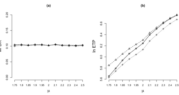
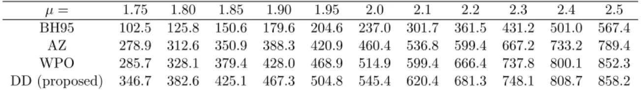
averaging results over 200 replications. The simulation results are summarized in Figure 2. We can see from Panel (a) that all methods control the wFDR at the nominal level 0.1 approximately (the BH95 method is very conservative and the result is not displayed). Panel (b) shows that the proposed methods dominates other competing methods; and the gain in power is more pronounced when the signals are weak. (The ETP increases rapidly with increased signal strength. For better visualization of results, we present the graph in a logarithmic scale. See Table 1 for results of the BH95 method, as well as the ETP levels in original scales.)

(a) µ wFDR 1.75 1.8 1.85 1.9 1.95 2 2.1 2.2 2.3 2.4 2.5 0.00 0.05 0.10 0.15 0.20 (b) µ ln ET P 1.75 1.8 1.85 1.9 1.95 2 2.1 2.2 2.3 2.4 2.5 5.6 5.8 6.0 6.2 6.4 6.6

Figure 2: Comparison under group-wise weights: ◦ WPO, 4 DD (proposed), and + AZ.

The efficiency gain of the proposed method is more pronounced when signals are weak.

5.2 General weights

In applications where domain knowledge is precise (e.g. spatial cluster analysis), divid-ing the hypotheses into groups and assigndivid-ing group-wise weights would not be satisfydivid-ing. This section investigates the performance of our method when random weights (ai, bi) are

generated from a bivariate distribution.

In the third simulation study, we test m = 3000 hypotheses with ai, the weights

as-sociated with the wFDR control, fixed at 1. We generate bi, the weights associated with

the power (or ETP), from log-normal distribution with location parameter ln 3 and scale parameter 1. The location parameter is chosen in a way such that the median weight is 3, similar to those in previous settings. We apply different methods with 200 replications.

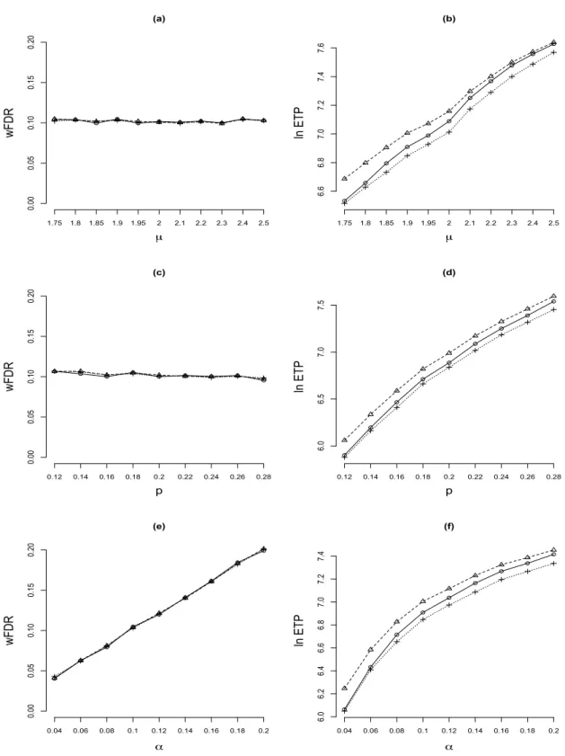
The simulation results are summarized in Figure 3. The first row fixes α = 0.10 and

p= 0.2, and plots the wFDR and ETP as functions of µ. The second row fixesα = 0.10 andµ= 1.9, and plots the wFDR and ETP as functions ofp. The last row fixesp= 0.2 and

µ= 1.9, and plots the wFDR and ETP as functions ofα. In the plots, we omit the BH95 method (which is very conservative) and present the ETP in a logarithmic scale (for better visualization of results). The following observations can be made: (i) all methods control the wFDR at the nominal level approximately; (ii) by exploiting the weightsbi, the WPO

method outperforms the unweighted AZ method; (iii) the proposed method outperforms all competing methods; (iv) Panel (f) shows that gains in power of the proposed method over the WPO method vary at different nominal levels α; (v) similar to the observations in previous simulation studies, the difference between the WPO method and the proposed method decreases with increased signal strength, the efficiency gain of the proposed method is larger as signals become more sparse.

Table 1: ETP values (in original scale) of various methods corresponding to Figure 2

µ= 1.75 1.80 1.85 1.90 1.95 2.0 2.1 2.2 2.3 2.4 2.5

BH95 102.5 125.8 150.6 179.6 204.6 237.0 301.7 361.5 431.2 501.0 567.4 AZ 278.9 312.6 350.9 388.3 420.9 460.4 536.8 599.4 667.2 733.2 789.4 WPO 285.7 328.1 379.4 428.0 468.9 514.9 599.4 666.4 737.8 800.1 852.3 DD (proposed) 346.7 382.6 425.1 467.3 504.8 545.4 620.4 681.3 748.1 808.7 858.2

In the last simulation study, ai’s are assigned to two groups of hypotheses with group

sizesm1= 3000 and m2 = 1500. In groups 1 and 2, we fix ai = 1 and ai = 3, respectively.

Conventional FDR methods are only guaranteed to work when allai are fixed at 1. Under

this setting, we expect that the unweighted AZ may fail to control the wFDR. We then generate random weightsbi from log-normal distribution with location ln 6 and scale 1. The

non-null proportion for group 1 is 0.2, and that for group 2 is 0.1. The mean of the the non-null distribution for group 1 orµ1 is varied between [−3.75,−2] while that for group 2

is fixed at 2. The simulation results are shown in Figure 4. We can see that the unweighted AZ method fails to control the wFDR at the nominal level, which verifies our conjecture. The observations regarding the ETP are similar to those in the previous simulation study. Overall, all numerical studies together substantiate our theoretical results and affirm the

(a) µ wFDR 1.75 1.8 1.85 1.9 1.95 2 2.1 2.2 2.3 2.4 2.5 0.00 0.05 0.10 0.15 0.20 (b) µ ln ET P 1.75 1.8 1.85 1.9 1.95 2 2.1 2.2 2.3 2.4 2.5 6.6 6.8 7.0 7.2 7.4 7.6 (c) p wFDR 0.12 0.14 0.16 0.18 0.2 0.22 0.24 0.26 0.28 0.00 0.05 0.10 0.15 0.20 (d) p ln ET P 0.12 0.14 0.16 0.18 0.2 0.22 0.24 0.26 0.28 6.0 6.5 7.0 7.5 (e) α wFDR 0.04 0.06 0.08 0.1 0.12 0.14 0.16 0.18 0.2 0.00 0.05 0.10 0.15 0.20 (f) α ln ET P 0.04 0.06 0.08 0.1 0.12 0.14 0.16 0.18 0.2 6.0 6.2 6.4 6.6 6.8 7.0 7.2 7.4

Figure 3: Comparison with general weights: ◦ WPO, 4 DD (proposed), and + AZ. All

methods control the wFDR approximately at the nominal level. The efficiency gains of the proposed method become more pronounced when (i) the signal strength decreases, (ii) the signals become more sparse, or (iii) the test levelα decreases.

(a) µ1 wFDR -3.75 -3.5 -3.25 -3 -2.75 -2.5 -2.25 -2 0.00 0.05 0.10 0.15 0.20 (b) µ1 ln ET P -3.75 -3.5 -3.25 -3 -2.75 -2.5 -2.25 -2 8.0 8.2 8.4 8.6 8.8

Figure 4: Comparison with general weights: ◦ WPO, 4 DD (proposed), and + AZ. The

unweighted AZ method fails to control the wFDR at the nominal level. The efficiency gain of the proposed method increases as signals become weaker.

use of the methodology in various settings.

6

Application to GWAS

Weighted FDR procedures have been widely used in GWAS to prioritize the discoveries in pre-selected genomic regions. This section applies the proposed method for analyzing a data set from Framingham Heart Study (Fox et al., 2007; Jaquish, 2007). A brief description of the study, the implementation of our methodology, and the results are discussed in turn.

6.1 Framingham Heart Study

The goal of the study is to decipher the genetic architecture behind the cardiovascular disorders for the Caucasians. Started in 1948 with nearly 5,000 healthy subjects, the study is currently in its third generation of the participants. The biomarkers responsible for

the cardiovascular diseases, for e.g., body mass index (BMI), weight, blood pressure, and cholesterol level, were measured longitudinally.

We analyze a subset of the original data set containing 977 subjects with 418 males and 559 females, whose BMIs are measured over time. Subjects are mostly from 29 years to 85 years old. The current data set also contains genetic information or genotype group of each participant over 5 million single nucleotide polymorphism (SNPs) on different chromosomes. Following the traditional GWAS, we exclude the rare SNPs, that is, SNPs with minor allele frequency less than 0.10, from our analyses. Male and Female populations are analyzed separately. For purpose of illustration, we only report the results from the Male population.

6.2 Multiple testing and wFDR control

We consider the BMI as the response variable and develop a dynamic model to detect the SNPs associated with the BMI. LetYi(tij) denote the response (BMI) from thei-th subject

at timetij,j= 1, . . . , Ti. Consider the following model for longitudinal traits:

Yi(tij) =f(tij) +βkGik+γi0+γi1tij+i(tij), (6.1)

wheref(·) is the general effect of time that is modeled by a polynomial function of suitable order,βk is the effect of thek-th SNP on the response andGikdenotes the genotype of the i-th subject for the k-th SNP. We also consider the random intercepts and random slopes, denoted γ0i and γ1i, respectively, for explaining the subject-specific response trajectories.

A bivariate normal distribution for γi = (γ0i, γ1i) is assumed. Moreover, we assume that

the residual errors are normally distributed with zero mean, and covariance matrix Σi with

an order-one auto-regressive structure.

We fit model (6.1) for each SNP and obtain the estimate of the genetic effectβb_k. If we

has a significant association with the BMI. Since we have nearly 5 million SNPs, the false discovery rate needs to be controlled for making scientifically meaningful inference. For eachk, we take standardizedβb_k as ourz-scores and obtain the estimated ranking statistic

b

Rk as described in (4.2). For selecting the weights, we use the following three methods,

withak= 1 in all the three cases:

Method I: Here we takebk= 1; this is just the unweighted case.

Method II: We first perform a baseline association test for each SNP. We consider only the baseline BMI for each subject and group the response values as High (BMI higher than 25), Low (BMI lower than 18.5), and Medium. For each SNP, we have three

genotypes and thus we get a 3 × 3 table for each SNP and perform a chi-square

association test. The p-values are recorded. Now we partition the SNPs into three groups based on these p-values (lower than 0.01, higher than 0.10, and in between). For each group, we compute the average of the inverse of thep-values and take this average asbk’s for all the SNPs belonging to this particular group.

Method III: We consider the dynamic model (6.1) and derive the p-values for testing

H0 : βk = 0 vs. H1 : βk 6= 0 for the Female population. We partition the SNPs

into three groups based on these p-values: lower than 0.01, higher than 0.10, and in between. For each group, we compute the average of the inverse of the p-values and take this average as the bk’s for all the SNPs belonging to this particular group

while analyzing the data from the Male population. Similar methodology of deriving weights from a reference population has been previously explored in Xing et al. (2010).

6.3 Results

In Table 2, we present the number of selected SNPs from three different methods at different

in GWA studies. In Table 3, we list some important SNPs (previously reported in the literature) detected by all three methods. For example, SNPs on chromosomes 3, 5, and 17 were reported in Das et al. (2011, Human Heredity) as significant SNPs associated with high blood pressure and related cardio-vascular diseases. SNPs on chromosome 6 and 8 were reported in Das et al. (2011, Human Genetics). Li et al. (2011, Bioinformatics) reported the SNP on chromosome 10 to be associated with BMI.

Table 2: Number of selected SNPs at different α levels for the Male population α Method I Method II Method III

10−3 1384 988 1093 10−4 _{832 447 518}

10−5 271 69 91 10−6 _{86 12 33}

Table 3: Some previously reported SNPs detected by all three methods

Chromosome SNP Position Trait/Disease (associated with) 3 ss66149495 16,140,422 Blood Pressure 5 ss66501706 147,356,971 Blood Pressure 6 ss66068448 131,562,687 BMI 8 ss66359352 11093585 BMI 10 ss66311679 32,719,838 BMI 17 ss66154967 29,846,491 Blood Pressure

In Table 4, we list previously reported SNPs which were detected only by Methods II and III. Das et al. (2011) reported the SNP on chromosome 12. Li et al. (2011) reported the SNPs on chromosomes 1, 10, 20, and 22.

Table 4: Some previously reported SNPs detected by Methods II and III only

Chromosome SNP Position Trait/Disease (associated with) 1 ss66185476 8,445,140 BMI

10 ss66293192 32,903,593 BMI 12 ss66379521 130,748,789 Blood Pressure 20 ss66171460 22,580,931 BMI 22 ss66055592 23,420,006 BMI

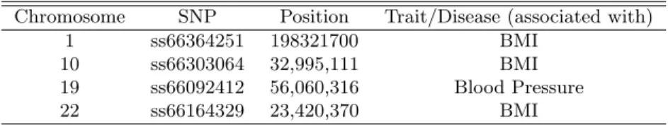
In Table 5, we list some previously reported SNPs which were detected only by Method III. Das et al. (2011) reported the SNP on chromosome 19. Li et al. (2011) reported the SNPs on chromosomes 1, 10, and 22.

Table 5: Some previously reported SNPs detected by Method III only.

Chromosome SNP Position Trait/Disease (associated with) 1 ss66364251 198321700 BMI

10 ss66303064 32,995,111 BMI 19 ss66092412 56,060,316 Blood Pressure 22 ss66164329 23,420,370 BMI

Note that 11 out of 12 SNPs identified by method II have been, as tabulated in Tables 3 and 4, previously identified in different studies. The SNP ss66077670 on Chromosome 9 is the only identified SNP that has not been previously reported, to our knowledge, and may be further explored by domain experts.

7

Discussion

In the multiple testing literature, procedural, decision, and class weights are often viewed as distinct weighting schemes and have been mostly investigated separately. Although this paper focuses on the decision weights approach, the decision-theoretic framework enables a unified investigation of other weighting schemes. For example, a comparison of the LR (3.8) and WLR (3.11) demonstrates how the LR statistic may be adjusted optimally to account for the decision gains/losses. This shows that procedural weights may be derived in the decision weights framework. Moreover, the difference between the WLR (3.11) and WPO (3.14) shows the important role that pi plays in multiple testing. In particular the WPO

(3.14) provides important insights on how prior beliefs may be incorporated in a decision weights approach to derive appropriate class weights. To see this, consider the multi-class model (2.3). Following the arguments in Cai and Sun (2009), we can conclude that in order to maximize the power, different FDR levels should be assigned to different classes. Similar suggestions for varied class weights have been made in Westfall and Young (1993, pages 169 and 186). These examples demonstrate that the decision weights approach provides a powerful framework to derive both procedural weights and class weights.

We have assumed that the decision weights are pre-specified by the investigators. It

is of interest to extend the work to the setting where the weights are unknown. Due

to the variability in the quality of external information, subjectivity of investigators, and complexity in modeling and analysis, a systematic study of the issue is beyond the scope of the current paper. Notable progresses have been made, for example, in Roeder and Wasserman (2009) and Roquain and van de Wiel (2009). However, these methods are

mainly focused on the weighted p-value approach under the unweighted FDR criterion,

hence do not apply to the framework in Benjamini and Hochberg (1997). Moreover, the optimal decision rule in the wFDR problem in general is not a thresholding rule based on the adjusted p-values. Much work is still needed to derive decision weights that would optimally incorporate domain knowledge in large-scale studies.

A

Appendix: Proofs

We prove all the technical results in this Appendix.

A.1 Proof of Theorem 1

Proof of Part (i). To show that wFDR(δδδOR) =α, we only need to establish that

EU,aaa,bbb,XXX ( _m X i=1 aiδORi (Lfdri−α) ) = 0,

where the notation EU,aaa,bbb,XXX denotes that the expectation is taken over U, aaa, bbb, and XXX.

According to the definitions of the capacity functionC(·) and threshold t∗, we have

m

X

i=1

It follows from the definition ofp∗ that E_U|aaa,bbb,XXX ( _m X i=1 aiδORi (Lfdri−α) ) =C(k) +{C(k+ 1)−C(k)}p∗ = 0,

where the notation EU|aaa,bbb,XXX indicates that the expectation is taken over U while holding

(aaa, bbb, XXX) fixed. Therefore EU,aaa,bbb,XXX ( _m X i=1 aiδORi (Lfdri−α) ) = 0, (A.1)

and the desired result follows.

Proof of Part (ii). Letδδδ∗ be an arbitrary decision rule such thatwF DR(δδδ∗)≤α. It follows that E_aaa,bbb,XXX ( _m X i=1 aiE(δi∗|aaa, bbb, xxx)(Lfdri−α) ) ≤0. (A.2)

The notation E(δ_i∗|xxx, aaa, bbb) means that the expectation is taken to average over potential randomization conditional on the observations and weights.

Let I+ _{= {i : δ}i OR−E(δ ∗ i|xxx, aaa, bbb) > 0} and I − _{= {i : δ}i OR−E(δ ∗ i|xxx, aaa, bbb) < 0}. For i∈ I+_{, we have δ}i

OR = 1 and hence bi(1−Lfdri) ≥t∗ai(Lfdri−α). Similarly for i∈ I−,

we have δi_OR= 0 and so bi(1−Lfdri)≤t∗ai(Lfdri−α). Thus

X

i∈I+_∪I−

δi_OR−E(δ∗_i|xxx, aaa, bbb) {bi(1−Lfdri)−t∗ai(Lfdri−α)} ≥0.

Note thatδ_ORi is perfectly determined byXXX except for (k+ 1)th decision. Meanwhile,

b(k+1) 1−Lfdr(k+1)

−t∗a(k+1) Lfdr(k+1)−α

by our choice oft∗. It follows that Eaaa,bbb,XXX " _m X i=1 E(δ_ORi |xxx, aaa, bbb)−E(δ_i∗|xxx, aaa, bbb) {bi(1−Lfdri)−t∗ai(Lfdri−α)} # ≥0. (A.3)

Recall that the power function is given by

ETP(δδδ) =E ( _m X i=1 E(δi|xxx, aa, bbba )bi(1−Lfdri) )

for any decision ruleδδδ. Combining equations (A.1) – (A.3) and noting thatt∗ >0, we claim that ETP(δδδOR)≥ETP(δδδ∗) and the desired result follows.

A.2 Proof of Theorem 2

A.2.1 Notations

We first recall and define a few useful notations. Let I_A be an indicator function, which equals 1 if eventA occurs and 0 otherwise. Let

Ni=ai(Lfdri−α), Nb_i =a_i(Lfdrd_i−α), Ri = ai(Lfdri−α) bi(1−Lfdri) +ai|Lfdri−α| , Rb_i= ai(Lfdrd_i−α) bi(1−Lfdrd_i) +a_i|Lfdrd_i−α| , Q(t) = 1 m m X i=1 NiIRi≤t and Qb(t) = 1 m m X i=1 b NiIRbi≤t fort∈[0,1].

Note that Q(t) and Qb(t), the estimates for oracle and data driven capacities, are

non-decreasing and right-continuous. We can further define

Next we construct a continuous version ofQ(·) for later technical developments. Specifically, for 0≤R_(k)< t≤R_(k+1), let Qc(t) ={1−r(t)}Q R(k) +r(t)Q R(k+1) ,

wherec indicates “continuous” andr(t) = (t−R_(k))/(R_(k+1)−R_(k)). LetR_(m+1)= 1 and

N(m+1) = 1. Similarly we can define a continuous version of Qb(t). For 0 ≤ Rb_(k) < t ≤ b

R_(k+1), let

b

Qc(t) = [1−_br(t)]Qb(Rb_(k)) +_br(t)Qb(Rb_(k+1)),

with_br(t) = (t−Rb_(k))/(Rb_(k+1)−Rb_(k)). Now the inverses ofQc(t) andQbc(t) are well defined;

denote these inverses by Qc,−1(t) and Qbc,−1(t), respectively. By construction, it is easy to

see that

IRi≤λOR =IRi≤Qc,−1(0) and IRbi≤bλ =IRbi≤Qbc,−1(0).

A.2.2 A useful lemma

We first state and prove a lemma that contains some key facts to prove the theorem.

Lemma 1 Assume that Conditions 1-3 hold. For any t∈[0,1], we have

(i) E b NiI_[Rb i≤t]−NiI[Ri≤t] 2 =o(1), (ii) E n b NiI_[Rb i≤t]−NiI[Ri≤t] NbjI[Rbj≤t]−NjI[Rj≤t] o =o(1), and (iii) Qbc,−1(0)−Qc,−1(0) p →0.

Proof of Part (i). We first decomposeENb_iI_[ b

Ri≤t]−NiI[Ri≤t]

2

into three terms:

E b NiI_[Rb i≤t]−NiI[Ri≤t] 2 = E[(Nb_i−N_i)2I b Ri≤t,Ri≤t] +E[Nb 2 iIRbi≤t,Ri>t] +E[N 2 iIRbi>t,Ri≤t]. (A.5)

Next we argue below that all three terms are ofo(1).

First, it follows from the definitions ofNb_i and N_i that

En(Nb_i−N_i)2I b Ri≤t,Ri≤t o =E a2_i Lfdri−Lfdrd_i 2 I b Ri≤t,Ri≤t ≤E a2_i Lfdri−Lfdrd_i 2 .

By an application of Cauchy-Schwarz inequality, we have

E a2_iLfdri−Lfdrd_i 2 ≤ E(a4_i) 1/2 ELfdri−Lfdrd_i 41/2 .

It follows from Condition 2 that E(a4_i) =O(1). To show E

Lfdri−Lfdrd_i 4

=o(1), note that both Lfdri and Lfdrd_i are in [0,1]. HenceE

Lfdri−Lfdrd_i 4

≤E|Lfdri−Lfdrd_i|. Using

the fact that Lfdri−Lfdrd_i =o_P(1), the uniform integrability for bounded random variables,

and the Vitali convergence theorem, we conclude that E|Lfdri−Lfdrd_i|=o(1). Therefore,

the first term in (A.5) is ofo(1).

Next we show that E

b N_i2I b Ri≤t,Ri>t

= o(1). Applying Cauchy-Schwarz inequality

again, we have ENb_i2I b Ri≤t,Ri>t ≤(1−α)2E(a4_i) 1/2nPRb_i≤t, R_i > t o1/2 .

Condition 2 implies that E(a4

i) =O(1); hence we only need to show that P(Rb_i ≤t, R_i > t) =o(1). Letη >0 be a small constant. Then

P(Rb_i ≤t, R_i> t) =P b Ri ≤t, Ri∈(t, t+η] +P b Ri ≤t, Ri> t+η ≤P(Ri ∈(t, t+η]) +P(|Rb_i−R_i|> η).

SinceRi is a continuous random variable, we can findηt>0 such thatP(Ri ∈(t, t+η])< ε/2 for a given ε. For this fixed ηt > 0, we can show that P(|Rb_i −R_i| > η_t) < ε/2 for

sufficiently large n. This follows from Lfdri−Lfdrd_i = o_P(1) and the continuous mapping

theorem. Similar argument can be used to prove that E[N2

iIRbi>t,Ri≤t] = o(1), hence

completing the proof of part (i).

Proof of Part (ii). AsXi andXj are identically distributed and our estimates are invariant

to permutation, we have E n (Nb_iI [Rbi≤t]−NiI[Ri≤t])(NbjI[Rbj≤t]−NjI[Rj≤t]) o ≤E b NiI_[Rbi≤t]−NiI[Ri≤t] 2 .

The desired result follows from part (i).

Proof of Part (iii). Define Q∞(t) = E(NiIRi≤t), where the expectation is taken over

(aaa, bbb, XXX, θθθ). Let

λ∞= inf{t∈[0,1] :Q∞(t)≤0}.

We will show that (i) Qc,−1(0) →p λ∞ and (ii) Qbc,−1(0)

p

→ λ∞. Then the desired result

b

Qc,−1(0)−Qc,−1(0)→p 0 follows from (i) and (ii).

Fix t ∈ [0,1]. By Condition 2 and WLLN, we have that Q(t) →p Q∞(t). Since

Qc,−1(·) is continuous, for any ε > 0, there exists a δ > 0 such that |Qc,−1(Q∞(λ∞))−

Qc,−1(Qc(λ∞))|< ε whenever |Q∞(λ∞)−Qc(λ∞)|< δ. It follows that

P{|Q∞(λ∞)−Qc(λ∞)|> δ} (A.6) ≥ P|Qc,−1(Q∞(λ∞))−Qc,−1(Qc(λ∞))|> ε

= P|Qc,−1(0)−λ∞|> ε . (A.7)

Equation (A.7) holds sinceQ∞(λ∞) = 0 by the continuity ofRi, andQc,−1(Qc(λ∞)) =λ∞ by the definition of inverse. Therefore we only need to show that for anyt∈[0,1], Qc(t)→p

Q∞(t). Note that

E|Q(t)−Qc(t)| ≤ E(supiai)

m →0,

by Condition 2. Using Markov’s inequality, Q(t)−Qc_{(t) →}p _{0. Following from Q(t) →}p Q∞(t), we have Qc(t)

p

→ Q∞(t). Therefore (A.6) and hence (A.7) goes to 0 as m → ∞, establishing the desired result (i)Qc,−1(0)→p λ∞.

To show result (ii)Qbc,−1(0)

p

→λ∞, we can repeat the same steps. In showingQc,−1(0)

p

→

λ∞, we only used the facts that (a) Q(t)

p

→ Q∞(t), (b) Qc,−1(·) is continuous, and (c)

Q(t)−Qc(t) →p 0. Therefore to prove Qbc,−1(0)

p

→ λ∞, we only need to check whether the same conditions (a) Qb(t)

p

→ Q∞(t), (b) Qbc,−1(·) is continuous, and (c) Qb(t)−Qbc(t)

p

→ 0

still hold. It is easy to see that (b) holds by definition, and (c) holds by noting that

E|Qb(t)−Qbc(t)| ≤

E(sup_iai) m →0.

The only additional result we need to establish is (a).

Previously, we have shown that Q(t)→p Q∞(t). Therefore the only additional fact that we need to establish is that|Qb(t)−Q(t)|

p

→0. Now consider the following quantity:

∆Q={Qb(t)−Q(t)} −[E{Qb(t)} −E{Q(t)}]. (A.8)

By repeating the steps of part (i) we can show that

|E{Qb(t)} −E{Q(t)}|=|E(N_iI_Ri≤t)−E(Nb_iI b Ri≤t)| →0. (A.9) By definition, ∆Q=m−1Pm i=1{Nb_iI_[ b Ri≤t]−NiI[Ri≤t]} −[E(NbiIRbi≤t)−E(NiIRi≤t)].For an

we need to show that var( m X i=1 {Nb_iI_[ b Ri≤t]−NiI[Ri≤t]})/m 2_→0.

Using the result in Part (i) we deduce that,

m−2Var ( _m X i=1 b NiI_[Rb i≤t]−NiI[Ri≤t] ) ≤m−2E ( _m X i=1 b NiI_[Rb i≤t]−NiI[Ri≤t] )2 = 1− 1 m E n b NiI_[Rb i≤t]−NiI[Ri≤t] NbjI[Rbj≤t]−NjI[Rj≤t] o +1 mE b NiI_[Rbi≤t]−NiI[Ri≤t] 2 =o(1).

It follows from the WLLN for triangular arrays that|∆Q|→p 0. Combining (A.8) and (A.9), we conclude that |Qb(t)−Q(t)|

p

→0, which completes the proof.

A.2.3 Proof of Theorem 2

Proof of Part (i). Consider the oracle and data driven thresholds λOR and bλ defined in

Equation (A.4) in Appendix A.2.1. The wFDRs of the oracle and data-driven procedures are wFDROR = E P i ai(1−θi)δi_OR E P i aiδi_OR , wFDRDD = E P i ai(1−θi)I_Rb i≤λb E P i aiIRbi≤bλ .

Making the randomization explicit, the wFDR of the oracle procedure is wFDROR= E m−1P i ai(1−θi)IRi≤λOR+m −1_a i∗(1−θ_i∗)δi ∗ OR E m−1P i aiIRi≤λOR+m −1_a i∗δi∗ OR ,

where i∗ indicates the randomization point in a realization. Note that both E{ai∗(1− θi∗)δi

∗

OR/m} and E{ai∗δi ∗

OR/m} are bounded by E(ai∗/m). Hence by Condition 2 both

quantities are ofo(1).

From the discussion in Appendix A.2.1,I_Ri≤λOR =IRi≤Qc,−1(0)andIRbi≤bλ =IRbi≤Qbc,−1(0). According to Part (iii) of Lemma 1, we have{Rb_i−Qbc,−1(0)} − {R_i−Qc,−1(0)} =o_P(1).

Following the proof of Lemma 1 that

E n ai(1−θi)IRb_i−Qbc,−1(0)≤0 o =Eai(1−θi)IRi−Qc,−1(0)≤0 +o(1). (A.10) It follows that m−1E{P iai(1−θi)IRbi≤bλ} →m −1_E{P iai(1−θi)IRi≤λOR}. Similarly, we

can show that

EaiIRbi−Qbc,−1(0)≤0

=E aiIRi−Qc,−1(0)≤0

+o(1). (A.11)

Further from Condition 2 the quantitym−1E(P

iaiIRi≤λOR) is bounded away from zero.

To see this, note that Condition 1 implies that ai is independent of Lfdri. It follows that

m−1E m X i=1 aiIRi≤λOR ! =E(aiIRi≤λOR)≥cpeα >0, (A.12)

where P(Lfdr(X) ≤ α) ≥ p_eα for some peα ∈ (0,1] for the choice of the nominal level α ∈(0,1) and X, an i.i.d copy of Xi. This holds for any non-vanishing α. (Note that all

hypotheses with Lfdri < αwill be rejected automatically). Therefore we conclude that

Proof of Part (ii). The quantity m−1ET PDD is defined as m−1E

biθiI_[Rbi≤λb]

. Making the randomization explicit, we have

m−1ET POR=E 1 m X i biθiI[Ri≤λOR]+ 1 mbi∗θi∗δ i∗ OR ! ,

wherei∗ indicates the randomized point. By Condition 2

0≤m−1Ebi∗θ_i∗δi ∗ OR ≤ Ebi∗ m ≤ Esup_ibi m =o(1).

From the discussion in Appendix A.2.1,IRi≤λOR =IRi≤Qc,−1(0) and IRbi≤bλ =IRbi≤Qbc,−1(0). Repeating the steps in proving the wFDR, we can show that

E biθiI_{[ ˆR} i≤λˆ] =E biθiI[Ri≤λOR] +o(1).

Finally, it is easy to show that E biθiI[Ri≤λOR]

≥ c(1−α)p_eα, which is bounded below

by a nonzero constant. Here the positive constantc is as defined in Condition 2 and p_eα is

defined immediately after (A.12). We conclude that ET PDD/ET POR = 1 +o(1) and the

proof is complete.

A.3 Proofs of Propositions

A.3.1 Proof of Proposition 2

Letλ >0 be the relative cost of a false positive to a false negative. Consider the following weighted classification problem with loss function:

Laaa,bbb(θθθ, δδδ) = m

X

i=1

We aim to findδδδ that minimizes the posterior lossEθθθ|XXX{Laaa,bbb(θθθ, δδδ)} argmin δ δ δ m X i=1 {λaiP(θi = 0|Xi)δi+biP(θi = 1|Xi)(1−δi)} = argmin δ δ δ m X i=1 {λaiP(θi = 0|Xi)−biP(θi= 1|Xi)}δi.

Therefore the optimal decision ruleδδδP F = (δP Fi :i= 1,· · · , m) is of the form

δi_{P F} =I aiP(θi= 0|Xi) biP(θi = 1|Xi) < 1 λ , (A.14)

which reduces to the test statistic defined in (3.14).

Next note that QP F(t) is a continuous and increasing function of t. Therefore we can

find tP F such that QP F(tP F) =α. For an arbitrary decision rule δδδ∗ ∈ Dα, we must have ET P(δδδ∗) ≤ ET P(δδδP F). Suppose not, then there exists δδδ∗ ∈ Dα such that PFER(δδδ∗) ≤ α= PFER(δδδP F) and−ETP(δδδ∗)<−ETP(δδδP F). Consider a weighted classification problem

with λ= 1/tP F. Then we can show that δδδ∗ has a smaller classification risk compared to δδδP F. This is a contradiction. Therefore we must have ETP(δδδ∗)≤ETP(δδδP F).

A.3.2 Proof of Proposition 3

Proof of Part (i). For convenience of notation, defineSi = 1/VCRi. We show that rankings

by increasing values ofRiandSiare the same. Ifi∈S+, then all values are positive. Sorting

by increasing Si is the same as sorting by decreasing (1/Si) + 1 and hence by increasing

1/(1/Si + 1), which is precisely sorting by increasing Ri. If i ∈ S−, then all values are

negative. Sorting by increasingSi is the same as sorting by decreasing (1/Si)−1 and hence

by increasing 1/(1/Si−1), which is again the same as sorting by increasingRi. The desired

Proof of Part (ii). The result follows directly from the facts that (a) Ri is negative when i∈S− and (b)Ri is positive ifi∈S+.

References

[1] Benjamini, Y., and Heller, R. (2007), “False Discovery Rates for Spatial Signals,” Jour-nal of the American Statistical Association, 102, 1272–1281.

[2] Benjamini, Y., and Hochberg, Y. (1995), “Controlling the False Discovery Rate: A Practical and Powerful Approach to Multiple Testing,” Journal of the Royal Statistical Society, Series B, 57, 289–300.

[3] Benjamini, Y., and Hochberg, Y. (1997), “Multiple Hypotheses Testing with Weights,” Scandinavian Journal of Statistics, 24, 407–418.

[4] Billingsley, P. (1991),Probability and Measure(2nd ed.), New York: John Wiley & Sons. [5] Box, G. E. P. (1950), “Problems in the Analysis of Growth and Wear Curves,”

Biomet-rics, 6, 362–389.

[6] Cai, T. T., and Sun, W. (2009), “Simultaneous Testing of Grouped Hypotheses: Finding Needles in Multiple Haystacks,” Journal of the American Statistical Association, 104, 1467–1481.

[7] Das, K., Li, J., Fu, G., Wang, Z., and Wu, R. (2011), “Genome-Wide Association Studies for Bivariate Sparse Longitudinal Data,” Human Heredity, 72, 110–120.

[8] Das, K., Li, J., Wang, Z., Tong, C., Fu, G., Li, Y., Xu, M., Ahn, K., Mauger, D., Li, R.,

and Wu, R. (2011), “A Dynamic Model for Genome-Wide Association Studies,”Human

Genetics, 129, 629–639.

[9] Efron, B. (2008), “Simultaneous Inference: When Should Hypothesis Testing Problems be Combined?” The Annals of Applied Statistics, 2, 197–223.