Learning from High-Dimensional Multivariate Signals.

(1)

Learning from high-dimensional multivariate

signals

by

Arnau Tibau-Puig

A dissertation submitted in partial fulfillment of the requirements for the degree of

Doctor of Philosophy (Electrical Engineering: Systems)

in The University of Michigan 2012

Doctoral Committee:

Professor Alfred O. Hero III, Chair Professor Anna Catherine Gilbert

Assistant Professor Rajesh Rao Nadakuditi Assistant Professor Clayton D. Scott

(2)

(3)

“Als meus pares, per haver-me donat el tresor de la vida i haver-me ensenyat a gaudir-ne.”

(4)

ACKNOWLEDGEMENTS

This work would not have been possible without the advice, guidance and patience of several individuals. Chief among them is Professor Hero, who has guided me throughout the last four years with dedication, and has taught me that, in research, there is always an aspect worth exploring in more detail, a paragraph deserving additional editing, or a proof waiting to be simplified.

At the beginning of this journey, I must confess, I was quite lost: geographically (after moving to a new country), climatically (Michigan’s January is quite different from Spain’s), and also intellectually (what to do with four years of research ahead!). Several people helped me relocate my spirit and my body, and contributed to the success of this project. By order of appearance, Ami Wiesel taught me how to start and, more importantly, how to finish my first conference paper, and also half of what I have learnt in convex optimization. My numerous other colleagues in the Hero Research Group (Mark Kliger, Patrick Harrington, Yongsheng Juang, Kevin Xu, Greg Newstadt, Yilun Chen, Kumar Shridharan, Sung Jin Huang, Fra Bassi, Denis Wei, Mark Shiao, Zaoshi Meng) made my arrival and my life at the University of Michigan much easier, both professionally and personally. On the other side of the Atlantic Ocean, Gilles Fleury, Laurent Le Brusquet and Arthur Tenenhaus made me feel at home during my summer stays at Supelec, France, and gave me valuable insight and comments during each of our frequent videoconferences.

At the University of Michigan, I have had the unvaluable opportunity to learn about Sparse Approximmation/Compressive Sensing and Random Matrix Theory from two of the leading experts in the field, Anna Gilbert and Raj Rao Nadakuditi, who gracefully accepted to sit in my dissertation committee. Together with Clayton Scott, they gave me insightful comments and advice towards the transformation of my dissertation proposal into the present document.

I would also like to express my gratitude to all the good friends I have made during the last years. I came to the US socially empty-handed, and I will probably leave with many life-long friends from whom I learnt and enjoyed a great deal. To those who gave me support during each of my winter crises: Cristina Reina and Ricardo Ferrera,

(5)

Nicolas Lamorte, Remy Elbez, Emilie Bourdonnay, Aghapi Mordovanakis, Myriam Affeiche, Paul Samaha, Hannah Darnton, Emmanuel Bertrand, Laith Alattar, Adrien Quesnel, Wylde Norellus, Sofiya and Jamie Dahman, Le Nguyen, German Martinez and Maria Vega, Rahul Ahlawat, Matt Reyes and Awlok Josan: Thanks to you all!

I would finally like to thank the many people from the Electrical Engineering and Computer Science department that are always willing to assist graduate students in need of help: Becky Turanski, Ann Pace, Michel Feldman, and the DCO team, whose members always managed to reply to my frequent demands within hours.

I can’t finish this section without dedicating a special paragraph to Maria Luz Alvarellos, who gently put up with me during the hard-working months that preceded my oral defense, always ready to give a word (or a kiss) of encouragement. Gracias, Maria Luz!

(6)

LIST OF FIGURES

Figure

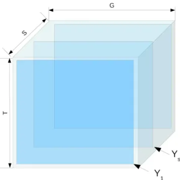
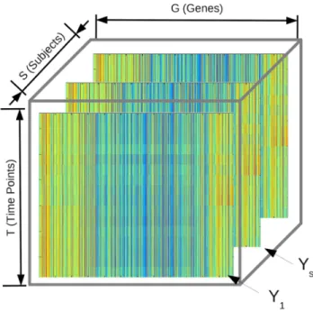
1.1 Multivariate signal data cube. . . 9 1.2 Predictive Health and Disease data cube. . . 11 1.3 Heatmap of the logarithm of the 11961 _×16 normalized temporal

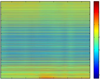
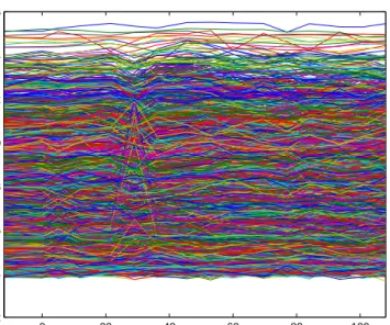
gene expression matrix for a subject inoculated by H3N2 (influenza). 12 1.4 Expression values for 5000 genes with high relative temporal

vari-ability over 16 time points for a subject inoculated by H3N2. Un-derlying temporal patterns are clearly not visible due to noise and high-dimensionality. . . 13 1.5 Construction of the factor matrix M(F,d) by applying a circular

shift to a common set of factors F parameterized by a vectord. . . 19 1.6 Estimated and true principal components, for 2 variables x1 and x2

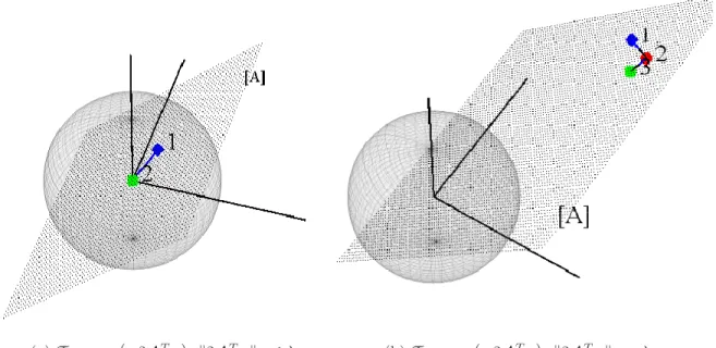
and 5 samples, and increasing SNR. It is clear that the PCA estimate is pretty accurate at 10dBs, while it is almost orthogonal to the true one at ₋3dBs. . . 22 2.1 Three-dimensional example of the result of applying the MSTO to

a vector y (denoted by (1) in the figure). The sphere (of radius λ) represents the boundary of the region in which ₋2ATy gets thresh-olded to 0, the plane represents the subspace [A]. Point (2) on the right plot is the projection of y onto [A] and point (3) is the pro-jected point after the shrinkage. Notice that as predicted by Theo-rem II.1, the amount of shrinkage is small compared to the norm of

Tλ,2AT_A

¡

−2ATy¢

, since the point ₋2ATy is far from the threshold boundary λ. . . 32

(10)

2.2 Comparison of Mosek®, MSTO and FISTA elapsed times for solving (2.27) while varyingp (withp/n= 1 fixed, plot (a)) and varyingp/n (with n = 100 fixed, plot (b)). For each algorithm, we compute the MSTO solution for three different values of the penalty parameterλ. MSTO is significantly faster than the other two when the conditioning of the problem is not too poor and offers comparable performance in the other regimes. . . 36 2.3 Comparison of prediction performances for the 2-class problem withp

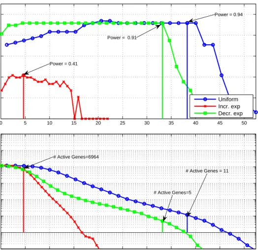
variables andn samples, for each of the methods discussed in Section 2.4.2: nearest shrunken centroid (PAM), nearest group-shrunken cen-troid (MSTO-PAM) and nearest group-shrunken cencen-troid using the approximation from (TP07) (MSTO-PAM Approx). The measure of performance is the estimated Area Under the Curve (AUC). As the number of samples increases, the advantage of M ST O−P AM and its approximation over PAM increases, possibly due to the incorpo-ration of the covariance within groups of variables in the predictor estimator. . . 40 2.4 Cross-validation results for the three choices of W. The top plot

shows the estimated power of our classifier versus λ. The bottom plot shows the average number of genes used in the classifier versus λ. As λ increases, the penalty is more stringent and the number of genes included in the model decreases. . . 42 2.5 Average within-class expression response and the bootstrapped 95%

confidence intervals for the significant genes (appearing in more than 70% of the CV predictors) obtained for each choice of weight matrix

W. W1 favors genes that are discriminative in the early time points,

which leads to poor prediction performances. On the contrary, W2

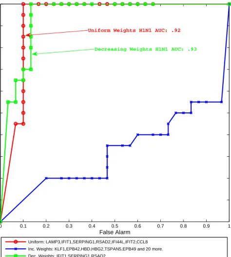
encourages a classifier that is highly discriminative at the late time points, which is where the difference between classes is stronger, lead-ing to high prediction performance. . . 44 2.6 Estimated ROC for predictors of Symptomatic/Asymptomatic

con-dition of H1N1-infected subjects, constructed from the sets of genes obtained in the H3N2 analyses. . . 45 3.1 Number of pathways containing each gene, for the subset of 5125

genes and 826 pathways used in the analyses of Section 3.4. On aver-age, each gene belongs to 6.2 pathways, and the number of pathways containing each gene ranges from 1 to 135. . . 47

(11)

3.2 Comparison of GSTO and FISTA (LY10; BT09) elapsed times for solving (3.30) as a function of p (a), m (b) and n (c). GSTO is significantly faster than FISTA for plarger than 4000 and small m. 67 3.3 Comparison of GSTO and FISTA (LY10; BT09) elapsed times for

computing the regularization path of (3.30) as a function of p(a), m (b) and n (c). GSTO is significantly faster than FISTA for p larger than 105 _{and small} _m, _{n. . . .} ₆₈

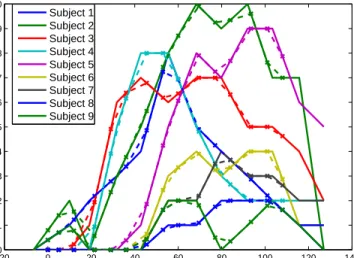
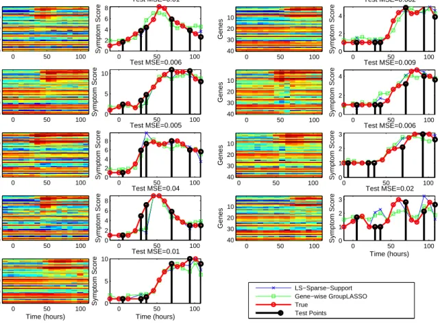
3.4 Interpolated (dashed) and original (solid lines) aggregated symptom scores for each of the H3N2 infected symptomatic individuals. . . . 70 3.5 Left columns: Heatmap of the gene expression values associated to

the active genes used in the predictor. Right columns: True and pre-dicted aggregated symptom scores for each individual. The predic-tors considered here are (i) the Gene-wise Group LASSO multi-task estimate (labeled as “Gene-wise GroupLASSO”) and (ii) the Least Squares predictor restricted to the support of the Gene-wise Group LASSO multi-task estimate (labeled as “LS-Sparse-Support”). The average relative MSE over the 9 subjects is 0.012. . . 74 4.1 Example of temporal misalignment across subjects of upregulated

gene CCRL2. Subject 6 and subject 10 show the earliest and the latest up-regulation responses, respectively. . . 77 4.2 Example of gene patterns with a consistent precedence-order across

3 subjects. The down-regulation motif of gene CD1C precedes the peak motif of gene ORM1 across these three subjects. . . 79 4.3 Example of gene patterns exhibiting co-expression for a particular

subject in the viral challenge study in (ZCV+_{09). . . .} ₈₀

4.4 Each subject’s factor matrix Ms is obtained by applying a circular

shift to a common set of factors F parameterized by a vectord. . . 82 4.5 Dictionary used to generated the 2-factor synthetic data of Section 4.4. 89 4.6 MSE (top) and DTF (bottom) as a function of delay variance σ2

d for

OPFA and Sparse Factor Analysis (SFA). These curves are plotted with 95% confidence intervals. For σ2

d > 0, OPFA outperforms SFA

both in MSE and DTF, maintaining its advantage as σd increases.

For largeσd, OPFA-C outperforms the other two. . . 92

4.7 Same as Figure 4.6 except that the performance curves are plotted with respect to SNR for fixed σ2

(12)

4.8 Comparison of observed (O) and fitted responses (R) for three of the subjects and a subset of genes in the PHD data set. Gene expression profiles for all subjects were reconstructed with a relative residual error below 10%. The trajectories are smoothed while respecting each subject’s intrinsic delay. . . 94 4.9 Comparison of observed (O) and fitted responses (R) for four genes

(OAS1, CCR1, CX3CR1, ORM1) showing up-regulation and down-regulation motifs and three subjects in the PHD dataset. The gene trajectories have been smoothed while conserving their temporal pat-tern and their precedence-order. The OPFA-C model revealed that

OAS1 up-regulation occurs consistently afterORM1 down-regulation among all subjects. . . 95 4.10 Top plots: Motif onset time for each factor (2) and peak symptom

time reported by expert clinicians (O). Bottom plots: Aligned factors for each subject. Factor 1 and 3 can be interpreted as up-regulation motifs and factor 2 is a strong down-regulation pattern. The arrows show each factor’s motif onset time. . . 96 4.11 The first two columns show the average expression signatures and

their estimated upper/lower confidence intervals for each cluster of genes obtained by: averaging the estimated Aligned expression pat-terns over the S = 9 subjects (A) and directly averaging the mis-aligned observed data for each of the gene clusters obtained from the OPFA-C scores (M). The confidence intervals are computed accord-ing to +/−the estimated standard deviation at each time point. The cluster average standard deviation (σ) is computed as the average of the standard deviations at each time point. The last column shows the results of applying hierarchical clustering directly to the original misaligned dataset _{Xs}S_s₌₁. In the first column, each gene

expres-sion pattern is obtained by mixing the estimated aligned factors F

according to the estimated scores A. The alignment effect is clear, and interesting motifs become more evident. . . 97

(13)

5.1 Predicted and average values ofλf(S(0)) and|hvf(S(0)),vf(Σ(0))i|2

, f = 1,_{· · ·} ,3, for H _∈ Rp×3 _{equal to three orthogonal pulses with}

narrow support (their support is much smaller than the dimension of the signal), shown in the top panel. The predictions of Theorem V.1 are shown in solid lines, the empirical average obtained over 50 random realizations are shown dashed. As p and n increase, the em-pirical results get closer to the predicted values. Notice that in this experiment the first three eigenvalues of the population covariance are close to each other, rendering the estimation of the correspond-ing eigenvectors harder. Figure 5.2 shows the results of the same experiment with pulses of larger width. . . 106 5.2 Same as in Figure 5.1 for H _∈Rp×3 _{equal to three orthogonal pulses}

with large support (their support is in the order of the dimension of the signal). Notice that in this case the eigenvalues of the popu-lation covariance are more spaced than in the results of Figure 5.1, as reflected by the distance between the phase transition points of each eigenpair, and the convergence of the empirical results to the predictions is faster. . . 107 5.3 Eigenvalues for the autocorrelation matrixRh for two 20-dimensional

signals: a rectangular and a triangular signal of increasing width, denoted by W, anddmax= 10. The upper and lower bounds for each

eigenvalue are computed using Theorem V.2. . . 112 5.4 Heatmaps depicting the average value over 30 random realizations of

the affinitya(HPCA_,_·_{) between the PCA estimate and the true signal,}

as a function of (SNR, dmax) (middle panel) or (SNR, n) (bottom

panel), for each of three rank-1 signals shown on the top panel. The red line corresponds to the computed phase transition SNR, given by Theorem V.1. The white dashed lines depict the upper and lower bounds obtained by combined application of Theorems V.1 and V.2. 121 5.5 Asymptotic bias for the PCA estimate of a misaligned rank 3 signal

of dimensionp= 300 with uniformly distributed misalignments of in-creasing magnitude. We consider three signals, depicted in the upper panels, with increasingly larger support. Our asymptotic predictions demonstrate the intuitive fact that signals with wider support are more robust to misalignments: the bias for the signal on the right-most plots is about one third of the bias for the narrow signal on the leftmost plots. . . 123

(14)

5.6 Estimated SNR levels needed for each of the algorithms to attain a level of fidelity ρ, defined as minnSNR :d³Hˆ,H´_≤ρo, for ρ _∈

, as a function of the number of samplesn, and as a func-tion of dmax, the maximum misalignment, for a rank-1 signal (F = 1). 125

5.7 Same as in Figure 5.6 for the case F = 3. Notices that since PCA is biased, here it fails to attain the target fidelity level in several regimes.126 5.8 Same as in Figure 5.6 for the case F = 10. . . 127 5.9 Right: MisPCA vs OPFA under a non-negative MisPCA generative

model. Left: MisPCA vs OPFA under an OPFA generative model. . 127 5.10 Hierarchical Clustering results obtained after MisPCA and

PCA-based dimensionality reduction. The leftmost and the right most pan-els show the centroids (+/₋standard deviations) after MisPCA and PCA, respectively. The middle panels correspond to a 2-dimensional embedding of the data projected on the MisPC’s (left) and the PC’s (right). . . 129 C.1 Right: Each subject’s factor matrix Mi is obtained by applying a

circular shift to a common set of factors F parameterized by a vec-tor of misalignment. d. Left: In order to avoid wrap-around effects when modeling transient responses, we consider instead a higher di-mensional truncated model of larger dimension from which we only observe the elements within a window characterized by Ω. . . 147 C.2 (a) Time point of interest (tI) for the up-regulation feature of factor

1. (b) The absolute time points t1,1, t1,2 are shown in red font for

two different subjects and have been computed according to their corresponding relative delays and the formula in (C.3). . . 148

(15)

LIST OF TABLES

Table

3.1 Comparison of symptom prediction performance for each of the Multi-task regression methods of Section 3.4.3. . . 70 3.2 Top-10 genes in the support of the Gene-wise Group-LASSO

multi-task predictor, ordered by ANOVA p-value. . . 72 3.3 Active pathways and their active genes (ordered by ANOVA p-value)

in the support of the Pathway-wise Group-LASSO multi-task pre-dictor. Highlighted in red are the genes that also appeared in the Gene-wise Group LASSO predictor. . . 73 4.1 Special cases of the general model (4.2). . . 77 4.2 Models considered in Section IV-A. . . 89 4.3 Sensitivity of the OPFA estimates to the initialization choice with

respect to the relative norm of the perturbation (ρ). . . 91 4.4 Cross Validation Results for Section 4.4.2. . . 94 5.1 Sensitivity of the A-MisPCA estimates to the initialization choice. . 128 5.2 Performance of the Brute Force MisPCA estimator. . . 128

(16)

LIST OF APPENDICES

Appendix A. Appendix to Chapter 2 . . . 136 B. Appendix to Chapter 3 . . . 138 C. Appendix to Chapter 4 . . . 146 D. Appendix to Chapter 5 . . . 154

(17)

NOTATION

The following notation convention is adopted throughout this dissertation. Bold-face upper case letters denote matrices, boldBold-face lower case letters denote column vectors, standard lower case letters denote scalars and standard upper case letters denote random variables. In addition, we define:

Sets and generalized inequalities:

R_{: the field of real numbers.} C_{: the field of complex numbers.}

Rp_{: the set of} _{p-dimensional real-valued vectors.}

Rp₊_{: the non-negative orthant, i.e., the set} _{_x_∈R_:_x_i _≥₀_}_. Rp

++: the positive orthant, i.e., the set {x∈R:xi >0}.

Rp×n_{: the set of} _p_×_n _{real-valued matrices.} Sp_{: the set of} _p_×_p _{symmetric matrices.} Sp

+: the subset of semi-positive definite matrices, i.e. Sp

+ =

©

X _∈Sp _:_xT_Xx_≥_0,_∀_x_∈Rpª_. Sp₊₊_{: the subset of positive definite matrices, i.e.}

Sp ++ = © X _∈Sp _:_xT_Xx_>_0,_∀_x_∈Rpª . xº0 (x≻0 ) means that x∈Rp₊ ₍_x_∈Rp₊₊_). X _º0 (X _≻0 ) means that X _∈Sp + (X ∈Sp++).

||·||2: the ℓ2 norm of a vector, ||x||2 =

pPp i=1x2i.

||·||F: the Frobenius norm of a matrix, ||X||F =

q Pp

i=1

Pn

j=1x2i,j.

Given a proper coneC ⊂Rp _and _x_,_y_∈Rp_, _x_º_C _y _{means that} _x₋_y_∈_C.

K: the second order (Lorentz) cone, K = ½· x t ¸ ∈RN+1 _:_||_x_|| 2 ≤t ¾ .

Matrix notation and operators:

T_{: matrix transpose operator.}

†_{: matrix pseudoinverse operator.} ⊗: Kronecker product.

(18)

[_·]_S,T: submatrix operator, returns the matrix constructed from the rows indexed byS and the columns indexed byT. We will drop the brackets whenever this is possible. Similarly, [·]_S,_∗ denotes the submatrix obtained from the row indices inS and all its columns.

diag (x) returns a diagonal matrix with the elements of x in its diagonal. tr (·): the trace operator.

det (_·): the determinant.

supp (X) returns the subset of column indices corresponding to columns with at least one non-zero element.

h·,_·i denotes the euclidean inner product between two matrices or vectors, de-fined as_hX,Y_i= tr¡

XTY¢.

(·)₊ denotes the projection onto the non-negative orthant.

R(X) denotes the range of a matrix X.

In is the n×n identity matrix.

0n×p and 1n×p denote then×pmatrices of all-zeroes and all-ones respectively.

We will omit the dimensions whenever they are clear from the context.

Spectrum of symmetric matrices

λi(X) and vi(X): thei-th eigenvalue and eigenvector of X ∈Sp.

λmax(X) andλmin(X) are defined as maxiλi(X) and miniλi(X), respectively.

ℵ(X) := _λλ_max(X)min(X) is the condition number of X _∈Sp_.

VF(X) and ΛF (X) denote thep×F matrix andF×F diagonal matrix obtained

from the firstF eigenvectors and the first F eigenvalues ofX _∈Sp_{, considering}

the eigenvalues in decreasing order andF ≤p.

Functions:

f(x): a generic real-valued function, f :Rp _→R_.

f(x): a generic multi-dimensional real function,f :Rp _→Rn_.

∇f: the gradient of a differentiable real-valued function,

∇f = · df(x) dx1 ,· · · ,df(x) dxp ¸T .

∇2_f_{: the Hessian of a twice-differentiable real-valued function,}

£ ∇2f¤ i,j = d2_f₍_x₎ dxidxj . For any two real-valued functions f(x), g(x), we write

f(x) = _O(g(x)) if lim sup x→∞ ¯ ¯ ¯ ¯ f(x) g(x) ¯ ¯ ¯ ¯ <_∞ f(x) = o(g(x)) if lim x→∞ f(x) g(x) = 0.

(19)

ABSTRACT

Learning from high-dimensional multivariate signals by

Arnau Tibau Puig

Chair: Alfred O. Hero III

Modern measurement systems monitor a growing number of variables at low cost. In the problem of statistically characterizing the observed measurements, budget limitations usually constrain the number n of samples that one can acquire, leading to situations where the numberpof variables is much larger thann. In this situation, classical statistical methods, founded on the assumption thatnis large andpis fixed, fail both in theory and in practice. A successful approach to overcome this problem is to assume a parsimonious generative model characterized by a number k of free parameters, wherek is much smaller than p.

In this dissertation we develop algorithms to fit low-dimensional generative models and extract relevant information from high-dimensional, multivariate signals. First, we define extensions of the well-known Scalar Shrinkage-Thresholding Operator, that we name Multidimensional and Generalized Shrinkage-Thresholding Operators, and show that these extensions arise in numerous algorithms for structured-sparse lin-ear and non-linlin-ear regression. Using convex optimization techniques, we show that these operators, defined as the solutions to a class of convex, non-differentiable, op-timization problems have an equivalent convex, low-dimensional reformulation. Our equivalence results shed light on the behavior of a general class of penalties that in-cludes classical sparsity-inducing penalties such as the LASSO and the Group LASSO. In addition, our reformulation leads in some cases to new efficient algorithms for a variety of high-dimensional penalized estimation problems.

Second, we introduce two new classes of low-dimensional factor models that ac-count for temporal shifts commonly occurring in multivariate signals. Our first

(20)

con-tribution, called Order Preserving Factor Analysis, can be seen as an extension of the non-negative, sparse matrix factorization model to allow for order-preserving tempo-ral translations in the data. We develop an efficient descent algorithm to fit this model using techniques from convex and non-convex optimization. Our second contribution extends Principal Component Analysis to the analysis of observations suffering from arbitrary circular shifts, and we call it Misaligned Principal Component Analysis. We quantify the effect of the misalignments in the spectrum of the sample covariance ma-trix in the high-dimensional regime and develop simple algorithms to jointly estimate the principal components and the misalignment parameters.

All our algorithms are validated with both synthetic and real data. The real data is a high-dimensional longitudinal gene expression dataset obtained from blood samples of individuals inoculated by different types of viruses. Our results demonstrate the benefit of applying tailored, low-dimensional models to learn from high-dimensional multivariate temporal signals.

(21)

CHAPTER I

Introduction

1.1 From petal lengths to mRNA abundance

The text-book famous “Iris flower dataset” (Fis36) was collected by E. Ander-son and was popularized by R.A. Fisher in 1936 to illustrate his method of Linear Discriminant Analysis. This dataset consists of 4 variables (Sepal length and width, Petal length and width) measured over 50 plants of three different species. To the 21st century statistics practitioner, a natural question is the following: if E. Ander-son’s intention was to characterize the morphological features of different species of Iris in a specific geographical area, why did he limit the number of variables to only four?

A plausible explanation is that E. Anderson was trying to strike a balance between the minimum number of features that could discriminate between species, and the number of different replicates he needed in order to obtain a representative sample. Since Anderson’s time budget for data collection was probably limited, measuring an additional feature would have likely implied a reduction in the total number of replicates for each feature.

Fisher and Anderson’s was an era where data collection was a manual or semi-automatized process, and the cost of measuring an additional variable was the same as the cost incurred in monitoring each of the previous ones. This was the data collection paradigm until the end of the 20th century: From medical research to communications systems, the number of measured variables was limited by the fact that the cost of the measurement system grew strongly with the number of observables. As a consequence, one had to limit the number of variables in order to allocate enough budget to the collection of replicates.

The advent of modern manufacturing techniques brought this limitation to an end. In essence, new technologies have allowed measurement and computing systems to do

(22)

economies of scale in the number of sensing devices. The cost of adding an additional measurement sensor decreases with the number of sensors already integrated, giving rise to measurement devices monitoring many orders of magnitude more variables than in the past1_.

This shift has profoundly changed the process of data collection and analysis: now it is not necessary anymore for the biologist, the astronomist, the marketing specialist or the antenna in the receptor of a communication system to know in advance what the relevant variables are in order to statistically characterize a physical process. Instead, one obtains measurements from a large pool of candidate features, and then relies on computational power to process the data and select the variables relevant to the study.

For example, in the data analysis problem that motivates this work, we are inter-ested in extracting gene expression temporal patterns that drive the immune system response of a cohort to upper respiratory tract viral infections. Unfortunately, the specific genes that are involved in this process are unknown. During most of the past century, we would have had to use medical and biological a priori knowledge to determine a pool of candidate genes related to immune response and then perform costly and sensitive gene expression assays for each of the tissue samples. In contrast, modern Affymetrix mRNA microarray technology allows us to monitor tens of thou-sands of genes at low cost, and extract relevant information exclusively from the data using modern statistical techniques.

Unfortunately, the increase in the number of variables has not been accompanied by a proportional increase in the number of replicates or samples that one is able to record. As an example, very few mRNA microarray-based gene expression studies collect more than tens of replicates, usually due to budget constraints. This phe-nomenon is not limited to situations where the ratio between the available budget and the cost of each sample caps the number of available replicates. For instance, in wireless communications or in internet traffic data analysis (LBC+_{06), the process}

under measurement is time-varying and hence one can only take few snapshots be-fore violating the usual stationarity assumption. In conclusion, modern data sets are usually characterized by having a much larger number of variables (denoted by p)

1

Quoting the great statistician Jerome H. Friedman (Fri01): “Twenty years ago most data was still collected manually. The cost of collecting it was proportional to the amount collected. [...] Now much (if not most) data is automatically recorded with computers. There is a very high initial cost [...] that is incurred before any data at all is taken. After the system is set up and working, the incremental expense of taking the data is only proportional to the cost of the magnetic medium on which it is recorded. This cost has been exponentially decreasing with time.”

(23)

than replicates (denoted by n). This has a number of statistical and computational consequences, which we briefly explore in the following section.

1.2 Finding needles in a haystack

As the great statistician and applied mathematician David Donoho wrote (Don00), “[...] we are in the era of massive automatic data collection, systematically obtain-ing many measurements, not knowobtain-ing which ones will be relevant to the phenomenon of interest. Our task is to find a needle in a haystack, teasing the relevant information out of a vast pile of glut.”

In other words, the naive intuition according to which “the more data, the bet-ter” seems to fail. For a fixed number of samples n, increasing the dimension of the observables, p, (by, say, adding more sensors to our measurement system) effectively increases the amount of data: p×n. However, following Donoho’s metaphor, an increase inp is equivalent to an increase in the size of the haystack which is not nec-essarily followed by an increase in the amount of needles. Indeed, there is practical and theoretical evidence (JL08; FFL08) showing that an increase in the ratio p_n some-times blurs or even completely suppresses the informative part of a noisy signal. This paradox is usually known as the “curse of dimensionality”. It is also worth mention-ing that there are other consequences of the p ≫n regime which have been dubbed the “blessing” (as opposed to the “curse”) of dimensionality. Indeed, recent results in probability and statistics show that there is much more structure in high dimen-sional random data than one would expect. Moreover, this structure only manifests itself in the high-dimensional setting, hence one can onlytake advantage of it in such regime. Examples of this phenomena are the concentration of measure (Mas07) of (well-behaved) functions of high-dimensional random variables around its mean, the convergence of the distribution of eigenvalues of large random matrices to a simple asymptotic distribution (Wig55), or the asymptotic uncorrelation phenomenon, by which large sequences of random variables behave as if their terms were uncorrelated, as the number of terms increases.

In order to overcome the curse of dimensionality, one popular approach is to as-sume that most physical phenomena can be characterized by only a few variables. For instance, in the Iris dataset example, E. Anderson knew, probably thanks to his training and experience, that petal and sepal dimensions are good discriminatory variables for the Iris subspecies. Among infinitely many other morphological features, E. Anderson chose those four in order to perform his study. In contrast, in modern

(24)

datasets one does not know a priori what the relevant features are, but it is often still reasonable to assume that only a handful of the variables, or low-dimensional lin-ear combinations of them, are relevant. For instance, in a seminal paper (GST+_99),

Golub et al. showed that only 50 genes out of 6817 screened genes sufficed to build a simple classifier that discriminated between acute lymphoblastic leukemia (ALL) and acute myeloid leukemia (AML). This practical assumption is sometimes philosoph-ically justified by the principle of parsimony, which is often (and perhaps wrongly) identified2 _{with Occam’s razor: “entia non sunt multiplicanda praeter necessitatem”}

(entities must not be multiplied beyond necessity.) Whether the parsimony assump-tion is accurate or useful to describe reality is an important epistemological quesassump-tion. In this dissertation we embrace K. Popper’s view (Pop02), who argues that simpler models are preferable because they are better testable and less likely to be falsifiable3_.

1.3 Parsimonious statistical models

Mathematically, the notion of parsimony is formalized by assuming a low-dimensional generative model. In statistical learning, this is equivalent to restricting the class of probability distributions that model the observations. In this dissertation we adopt a parametric approach, which implies that the distribution classes we consider are com-pletely characterized by a finite-dimensional set of parameters. Denoting bypy(x;θ)

the joint distribution of a multivariate observationy _∈Rp_{, we will assume that:}

py(x;θ)∈ ½ f(x,θ) :R2p _→R₊_, Z f(x,θ)dx= 1,θ_{∈ M} ¾ , (1.1)

where M ⊂ Rp _{is the parameter space, which we assume to be a low-dimensional}

manifold of Rp_{. This characterization of the observations is theoretically attractive}

because for many families ofM and f(x,θ), the problem of estimatingθ is compu-tationally tractable and amenable to mathematical analysis. We proceed to illustrate a few instances of this general model that will appear throughout this dissertation.

Sparse Generalized Linear models: Generalized Linear Models (GLM) are su-pervised learning models that characterize the distribution of a label or response

2

In fact the history of what is often called “Occam’s razor” might have a funny twist. W.H. Thorburn thoroughly argues in (Tho18) that “Occam’s Razor is a modern myth. There is nothing medieval in it [...]”. According to (Tho18), the often-quoted latin statement was never written by Occam and was first utilized much later, in 1639, by John Ponce of Cork.

3

“Simple statements [...] are to be prized more highly than less simple ones because they tell us more; because their empirical content is greater; and because they are better testable.” Chapter 7, Section 43 in (Pop02)

(25)

variable y as a function of a set of covariates, denoted by x_∈Rp_{. In a}

Gener-alized Linear Model, py,x(y,x) is assumed to belong to the exponential family,

and the mean of the response variable y is modeled as: E(y_|x) =g−1¡

xTθ¢

where g(x) is called the link function and θ _{∈ M} are the model parameters. The estimation of θ is usually done by maximizing the likelihood of y given

x. In our context, we are interested in sparse GLMs, which means that _M specializes to:

Mk−sparse ={θ ∈Rp :||θ||0 ≤k} (1.2)

where we define:

||θ_||₀ :=|supp (θ)|,

and hence k is an upper bound on the number of non-zero elements in the parameter vector. The estimate of θ in Sparse GLMs has to verify the model constraints, which leads to a constrained Maximum Likelihood (ML) problem. Given a collection of n independent observations _{yi,xi}ni=1, the constrained

ML estimator of θ is defined as: ˆ θ:= arg max n X i=1 py|x(yi,xi). (1.3) s.t. _||θ_||₀ _≤k

In this work we consider two types of generalized linear models, the linear regression and the logistic regression model. In the linear regression model, g(x) is taken to be the identity andpy|x(y,x) is the Gaussian distribution with

unit variance. In such case, the ML estimate of θ is given by: ˆ θ = arg min n X i=1 ¯ ¯y_i−xT_i θ ¯ ¯ 2 (1.4) s.t. ||θ||0 ≤k,

(26)

appear-ing in inverse problems or compressive sensappear-ing (Tro06): ˆ

θ = arg min||y₋Dθ_||2₂ (1.5) s.t. _||θ_||₀ _≤k.

Here D is a matrix of dictionary elements (a basis or an overcomplete dictio-nary) andθ is the representation of the signal over this dictionary.

The second class of GLMs we will consider is the logistic regression model, where py|x(y,x) is the binomial distribution and g(x) is the logit function (HTF05).

In this case, the constrained MLE takes the form: ˆ θ= arg min n X i=1 yixTi θ−log ³ 1 +exTiθ ´ (1.6) s.t. ||θ_||₀ _≤k,

We will consider variants of these Sparse GLM’s in Chapter 2 and 3, in the application of finding groups of genes that discriminate the temporal responses over different populations.

Low-rank factor models: The models considered in the last section characterized a response variabley as the output of a sparse linear model:

y _≈Dθ ,||θ_||₀ _≤k,

where θ _∈ Rp _{is sparse but} _D _∈ _Rn×p _{is usually full column rank and/or}

overcomplete, withpmuch larger thann. In contrast, in this section we consider low rank linear models of the type:

y=F aT +n, rank (F) =f ≪p,

where p is the dimension of y, F _∈ Rp×f _{is a low-rank matrix of factors with}

rank much smaller than the dimension of the ambient space, a_∈Rf _{is a vector}

of coefficients and n _∈ Rp _{is a small, random residual error. Depending on}

the nature of the coefficient vector a and the residualn, this model specializes to different paradigms. For instance, if a and n are assumed to be zero-mean Gaussian random vectors, with isotropic covariance and unit variance, we have

(27)

that: py(x;Σ) = 1 √ 2π_|Σ_|1/2 exp µ −1 2x T_Σ−1_x ¶ , Σ∈ Mf−rank, where Mf−rank = © Σ_∈Rp×p :Σ=F FT +I _≻0,rank (F) =fª , (1.7)

which is a low-dimensional subset of the cone of positive definite matrices. This model is also known as the Probabilistic PCA model (TB99). We will adapt a similar model to the problem of estimating temporal patterns from misaligned signals in Chapter 5.

Another class of low rank models stems from the assumption that a is non-random parameter of interest. In this case, assuming the residual nis centered and normal with isotropic covariance, we have

py(x;H,a) = 1 p 2πσ2 n exp µ − 1 2σ2 n ¡ x₋HaT¢T ¡ x₋HaT¢ ¶ , ( H _{∈ M}H ⊂Rp×f a_{∈ M}a .

Under this model, a common estimate ofH and afrom observations _{yi}n_i₌₁ is

the constrained Maximum Likelihood Estimator, defined as: ˆ θ = arg min n X i=1 ¯ ¯ ¯ ¯y_i−HaT_i ¯ ¯ ¯ ¯ 2 (1.8) s.t. ( H ∈ MH ai ∈ Ma, i= 1,· · · , n.

Depending on the specific choice of_MH andMathis problem relates tok-means

clustering (HTF05), Sparse Coding/Dictionary learning (OF97; KDMR+_03),

Non-Negative Matrix Factorization (LS99a) or Tensor Decomposition (KB09), to name a few. We develop a special instance of this class of models in Chapter 4, in the problem of estimating order-preserving temporal factors from longitudinal gene expression data.

In this dissertation we propose three different low-dimensional models for the analysis of high-dimensional, multivariate signals which are extensions or

(28)

combina-tions of the models listed above. Our models build on the special characteristics of high-dimensional multivariate signals, which we proceed to describe in the following section.

1.4 The special flavor of (high-dimensional) multivariate

sig-nals

We define a multivariate signal as a finite collection of multivariate random vari-ables indexed by a set of increasing real numbers:

©£

Y₁t, Y₂t,· · · , Y_Gt¤

∈RG_{, t}_{∈ {{}_t₁_,_{· · ·} _{, t}_T_}_{, t}_i _≤_t_i₋₁_,₁_≤_i_≤_T_}ª _(1.9)

We will generally denote the realizations of the random variables (1.9) at a specific time point t by a row vector yT

t. A realization of the multivariate signal will be

identified with a T ×G matrix:

Y =       yT 1 yT 2 · · · y_TT       . (1.10)

In general, we will work with a collection of S realizations of (1.9), which we identify with the vertical slices of a data cube, denoted by{Ys}Ss=1 and shown in Figure 1.1.

The main difference between a multivariate signal and an ordinary collection of multivariate random vectors is the existence of an ordered structure,ti ≤ti−1,1≤i≤

T4_{. The order assumption is important because it is closely related to the correlation}

structure of Yt

i. Indeed, many time-varying physical processes exhibit some kind of

regularity over time: continuity, smoothness or other. For example, in video data, one expects a certain degree of continuity between the images of adjacent frames. Another example is gene expression longitudinal data, e.g., the one we describe in the next section, where the expression values of a given gene are not expected to change abruptly across adjacent time points. Statistically, this regularity manifests itself in the form of a temporal correlation betweenYit and its temporal neighborsYit−1,Yit+1,

· · ·,Y_it+f. If we are to learn a statistical model from realizations _{Ys}Ss=1, it seems

reasonable to enforce these properties in our estimators.

4

This is more generally the definition oflongitudinal data, which includes time series, spatial and others types of data.

(29)

Figure 1.1: Multivariate signal data cube.

From the discussion above, it follows that we can interpret multivariate signals as a class of multivariate random variables for which we have a regularity prior along (at least) one of the dimensions. Unfortunately, this prior comes at the price of a type of sensitivity that is seldom taken into account. In many situations, one can not obtain replicates _{Ys}n_i₌₁ from (1.9), but rather a transformed version of them,

Xs=Ts(Ys). (1.11)

It is obvious that except for the case where_Ts(·) is the identity operator, the statistical

properties of Xs will be different from those of5 Ys. Consequently, any estimator

building on the temporal regularity of the underlying signal can be severely affected by operators that modify its temporal correlation structure, such as permutations or simple cyclic translations. More generally, the statistical properties of the signal along the time axis are not invariant to transformations that alter its ordered structure. We propose in this thesis two models that seek to compensate for the effects of two classes of transformations Ts(·) that commonly occur in practice. In Chapter 4, we

consider a transformation model that applies order-preserving circular shifts to the

5

This is in general the case whenever the statistical properties ofYsthappen to be invariant with

(30)

basis elements of a generative linear model. In Chapter 5, we consider the simpler class of cyclic translation operators, in which case_Ts(·) is a permutation matrix. This

is a special case of the order-preserving model of Chapter 4, in which the shifts on each basis element are assumed to be the same.

There is another aspect of multivariate signals that we have not yet explored, and that has to do precisely with the “multivariate” part of the nomenclature. In many situations, the random variables Yt

i represent particular features of a large complex

system and hence correlation will exist not only along neighboring time points, but also across its multivariate structure (without restriction to neighboring indices in this case). For example, in the context of gene expression data analysis, it is well known that groups of genes belonging to the same signaling pathway exhibit similar expression patterns. Another example arises in the context of MIMO communication systems, which use correlation across signals received in different antennas at the receiver to take advantage of spatial diversity.

If one has such prior knowledge, it would be foolish not to use it to our advantage. In Chapter 2 and 3, we develop efficient optimization schemes to fit classes of Sparse GLMs that enforce a low-dimensional model constructed from a-priori knowledge of the underlying correlation structure.

We turn now to the description of the dataset which motivates most of the devel-opments in this work.

1.5 Predictive Health and Disease (PHD)

Despite its relatively low mortality rate, Acute Respiratory Infections such as Rhi-novirus (HRV), influenza (H3N2 and H1N1A), and respiratory syncytial virus (RSV) have an important societal and economical impact (ZCV+_{09). Today’s detection and}

classification of this family of diseases is largely based on physicians’ diagnostic exper-tise, which relies on the assessment of the symptoms displayed by infected individuals. The DARPA-funded Predictive Health and Disease project6 _{aims at developing novel}

detection and classification schemes for such pathologiesbefore the symptoms appear, through the measurement of a pool of mRNA abundances in peripheral blood. The underlying assumption is that peripheral blood is a good proxy for the immune sys-tem response of an individual to a viral entity, which starts hours before symptoms appear.

6

http://www.darpa.mil/Our_Work/DSO/Programs/Predicting_Health_and_Disease_(PHD) .aspx

(31)

In order to study the feasibility of the project’s goal, the PHD gene expression data set was collected as follows. After receiving appropriate Institutional Review Board approval, the authors in (ZCV+_{09) performed separate challenge studies with}

two strains of influenza (H3N2 and H1N1), human rhino virus (HRV) and respiratory syncytial virus (RSV). For each such challenge study, roughly 20 healthy individuals were inoculated with one of the above viruses, and blood samples were collected at regular time intervals until the individuals were discharged. The blood obtained at each of these time points was assayed with Affymetrix Genechip mRNA microarray technology, yielding a matrix of gene expression values for each subject, such as the one depicted as a heatmap in Figure 1.3. Stacking each subject’s gene expression matrix yields the data cube in Figure 1.2.

Figure 1.2: Predictive Health and Disease data cube.

The raw Genechip array data was pre-processed using robust multi-array analysis (IHC+_{03) with quantile normalization (BIAS03). For each of the individuals and}

each time point, experienced physicians determined whether symptoms existed and correspondingly assigned a set of labels. These labels constitute the ground truth for our supervised learning tasks.

In this dissertation we address two major statistical challenges arising from the PHD project goals. The first one, which we address in Chapters 2 and 3, is to determine which genes are discriminatory of the different states of disease progression,

(32)

Time (hours) Genes 0 20 40 60 80 100 1000 2000 3000 4000 5000 6000 7000 8000 9000 10000 11000 6 7 8 9 10 11

Figure 1.3: Heatmap of the logarithm of the 11961×16 normalized temporal gene expression matrix for a subject inoculated by H3N2 (influenza).

by using only early time samples with respect to the onset time, which is the time when the first symptoms are recorded. The number of samples available for this purpose is equal to the number of symptomatic subjects S = 9 times the number of time points used to train our predictors, which is smaller or equal than T = 16. On the other hand, the number of genes under our normalization scheme is equal to G = 11961, meaning that in this tasks we are in a high dimensional regime, where

# variables

# samples = SG×T ≥83.

Our second challenge, which we undertake in Chapters 4 and 5, is to discover temporal gene expression patterns that characterize the immune system response to viral infection. A quick glimpse at Figure 1.4, which plots the normalized expression values of 5000 genes with high temporal variability for a subject inoculated with H3N2, demonstrates that this is not an easy feat. In addition, as we will explore in Chapter 4, there is evidence that the immune system responses of each individual have different latencies, and hence the matricesXs corresponding to each subject can

not be taken as realizations from the same multivariate distribution. Instead, it will be convenient to model the observationsXsas in (1.11), where they are characterized

as the result of applying a certain transformation to the common, underlying immune system expression response denoted byYs.

We outline next the contributions of this dissertation towards achieving the afore-mentioned goals.

(33)

0 20 40 60 80 100 2 4 6 8 10 12 14 16 Time (hours)

Gene expression level

Figure 1.4: Expression values for 5000 genes with high relative temporal variability over 16 time points for a subject inoculated by H3N2. Underlying tempo-ral patterns are clearly not visible due to noise and high-dimensionality.

1.6 Structure of this dissertation

In this section we relate the different chapters of this dissertation to the statisti-cal learning problems associated to the Predictive Health and Diagnose project and dataset described above.

1.6.1 Penalized estimation and shrinkage-thresholding operators

We have seen in Section 1.2 that a number of estimation and approximation problems can be posed as a constrained optimization problem of the form:

ˆ

xiªn_i₌₁,θ¢, s.t. θ _{∈ M ⊂}Rp

where L(·,·) is usually a smooth and convex loss function measuring the fit of the data to the model parameterized byθ,_{xi_}n_i₌₁are independent, identically distributed samples, and _M denotes the subset of Rp _{characterizing the model constraints. In}

(34)

For instance, when _L is the squared ℓ2 loss,

L({xi}ni=1,θ) = n X i=1 ¯ ¯ ¯ ¯ ¯ ¯x i 1− h xi 2 xi3 · · · xip i θ¯¯ ¯ ¯ ¯ ¯ 2 2

the solution to (1.12) yields the bestk-sparse least squares approximation ofx1 from

x2, x3,· · · , xp. It is reasonable to think that such an estimator would have better

statistical properties than the unconstrained least squares (LS) estimator, specially in the high dimensional setting wherep > nand the least squares estimator is known to be inconsistent. (Note for instance that we can add any vector from the null-space of the design matrix to the LS solution without modifying the LS objective value).

Unfortunately, (1.12) is a combinatorial problem even when L(·,·) is the squared ℓ2 loss, and no efficient computational method is known to solve it. In fact, it is

known that the related problem of finding the smallest sparse approximation of a linear system is NP-Hard (Nat95).

One approach to circumvent the computational burden of solving (1.12) is to relax the combinatorial constraint _||θ_||₀ _≤ k to a convex constraint of the form _||θ_||₁ _≤τ (TBM79; Tib96; Tro06). Then one usually considers the penalized version of the constrained problem7_:

ˆ

xiªn_i₌₁,θ¢+λ_||θ_||₁ (1.13) where λ is a parameter in one-to-one relationship with the sparsity parameter τ. Since the loss function _L is usually convex (as in the GLM examples of Section 1.2), then (1.13) is a convex optimization problem. This seemingly simple relaxation has two surprising properties: (i) it transforms a combinatorial problem to a polynomi-ally solvable one (for instance, by interior point methods which are known to have polynomial time complexity for self-concordant objectives (Wri)), and (ii) it has been shown that under relatively mild assumptions the solution to (1.12) and the solution to (1.13) are very close (Tro06).

7

One can formalize the equivalence between the constrained and the penalized problems through Lagrange duality theory (BV).

(35)

The worst-case polynomial complexity of (1.13) represents a huge advantage with respect to the combinatorial nature of (1.12). Notwithstanding, in most modern statistical problems the dimension of the optimization domain, denoted byp, is often in the order of the tens or hundreds of thousands of variables. This precludes the usage of interior point (IP) methods which require the storage of p _×p matrices and the solution of p-dimensional systems of equations. Numerous efforts have been devoted to developing algorithms that are better adapted to this large-dimensional regime. Roughly speaking, these algorithms sacrifice the fast convergence properties of IP methods in exchange of a very low per-iteration cost and sometimes weaker convergence guarantees8 (DDDM04a; WNF09; CW06; BT09; BBC09).

In addition, the appropriate value of τ (or λ) is usually not known in advance. A common approach is to estimate this tuning parameter via cross-validation (HTF05), which requires the computation of the entire solution path, that is, the solution to (1.13) as a function of λ. For the least squares loss, homotopy algorithms (OPT00; EHJT04) take advantage of the piece-wise linearity of the solutions to (1.13) with respect to λ to efficiently compute the solution path at little cost.

The LASSO problem, which is the specialization of (1.13) to the least squares loss, has been proved effective for a variety of applications (MB06; THNC02; Can06). However, it is well known that consistency of the LASSO estimator is only possi-ble under low correlation conditions which are not necessarily reasonapossi-ble in practice (Bac08; NRWY10). To overcome this limitation, there has been a push to incorpo-rate penalties that enforce structures other than simple sparsity while maintaining the convexity of the optimization problem. One way to incorporate these structures is to consider a generalization of theℓ1 penalized estimation problem which takes the

following form:

ˆ

xiªn_i₌₁,θ¢+λΩ (θ), (1.14) where Ω (θ) is a sparsity-inducing penalty defined as:

Ω (θ) = m X i=1 √ ci||θGi||2, (1.15)

where ci >0, and Gi are subsets of indices such that Gi ⊆ {1,· · · , p} and ∪mi=1Gi =

{1,_{· · ·} , p_}. This class of penalties enforce more fine-grained sparse models, in that

8

By weak convergence we refer here to convergence of the sequence of objective values but not necessarily of the optimization parameters.

(36)

they require the complement of the support set of the solution ˆθ to be the union of the groups of active subsets:

supp³θˆ´={1,· · · , p} \ ∪i∈AGi, (1.16)

for some A ⊆ {1,· · · , m}. When the groups are formed by individual indices, prob-lem (1.14) specializes to the LASSO estimator, otherwise it is generally known as the Group LASSO, with (ZRY09; SRSE10b; JMOB10) or without overlap (YL06a). There is practical and theoretical evidence that such penalties are statistically su-perior to the ℓ1 approach when the correlation structure of the data and the

struc-ture of the sparsity enforced by the penalty agree (OWJ08; SRSE10a; JOB10). It is worth mentioning, however, that this class of penalties is by no means exhaus-tive and that other schemes based on different convex functionals have been devised (Bac10; JOV09; CT07; NW08).

Unfortunately, the increase in modeling possibilities brought about by the penal-ties in (1.15) is accompanied by an increase in the computational burden for solving the associated penalized learning problem (1.14). On one hand, the proximal operator associated to the penalty (1.15), defined as:

Pτ,Ω(x) = min θ 1 2τ ||θ−x|| 2 2+ Ω (θ), (1.17)

which constitutes the main building block for fast first order algorithms such as those in (ABDF11; WNF09; CW06; BT09; BBC09), is only easy to evaluate in theseparable

case, where the supports of the groupsGi do not overlap, or in thehierarchical case,

where the supports only overlap in a hierarchical manner. On the other hand, in general, the solutions to (1.14) are no longer linear with respect to λ, rendering the computation of the entire regularisation path more computationally demanding than in the ℓ1 case.

In the second and third chapter of this dissertation we address the aforementioned problems. First, we consider a generalization of (1.15) that incorporates the possibility of enforcing sparcity in a different coordinate system than the one where the regression fit is performed. This class of penalties is of the form:

Ω (θ) = m X i=1 √ ci||AGi,·θ||2, (1.18)

(37)

(GSTO):

Tλ,H(g) = arg min 1₂θTHθ+gTθ+λPm_i₌₁ci||AGi,·θ||₂. (1.19) In Chapter 2 and 3 we show that the GSTO arises naturally in a number of algorithms for group-sparse penalized linear and non-linear regression. For example, if AGi,· are indicator matrices such that [AGi,·]_i,i = 1, [AGi,·]_k,l = 0 for k, l 6= i, and we let

H =XTX,g =₋XTy, this problem specializes to theℓ1 penalized linear regression

problem (1.13). Other choices of AGi,· lead to group sparse solutions as in (1.16). More generally, in analogy to the Scalar Shrinkage Thresholding Operator (SSTO), the GSTO shrinks or thresholds the input vector g and returns a thresholded vector in the following sense:

Tλ,H(g)∈Ker (AD,·) (1.20)

where D = _∪i∈AGi for some active set A ⊆ {1,· · · , m}. In addition, we show that

the convex, non-differentiable problem (1.19) is approximately equivalent to a smooth (differentiable) optimization problem over a much smaller domain of dimensionm(as opposed top). This reformulation leads to efficient evaluations of Overlapping Group LASSO problem and the proximal operator (1.17), which in some cases outperform state-of-the-art first order methods. Finally, the smoothness of our reformulation over the active set of variables allows us derive first-order updates with respect to perturbations in λ, which enhance the computation of the regularization path over a grid of penalty parameters.

1.6.2 Order-Preserving Factor analysis

We have seen in Section 1.2 that one possible way to avoid overfitting in the high-dimensional regime is to enforce a low high-dimensional model. In unsupervised learning tasks, such as the one of extracting immune system-related temporal responses from gene expression data, a popular approach is to find a simultaneous factorization of the temporal slices of the data cube in Figure 1.2:

Ys ≈F As, s= 1,· · · , S. (1.21)

Here F is a T ×F factor (or loading) matrix common to all observations and As ∈

RF×G _{are the coordinates or scores of the} _{s-th observation on the factor matrix.}

(38)

over a test set of entries that were treated as missing during the training phase. In the application of this model to the gene expression example, F contains the temporal patterns that explain away the correlations between different genes, and eachAs describes the association of each subject’s genes with the temporal patterns

in F. Such a simultaneous matrix decomposition achieves several goals: it enhances interpretability, it reduces the variance due to noise and it can be useful in imputating potentially missing entries. The underlying assumption here is that there is strong correlation among the columns of Ys, and that this correlation is persistent for all

s= 1,· · ·, S, hence a few prototype patterns constructed from the columns of F are enough to approximate well the data. This is a reasonable assumption for multivariate signals, as we explained in Section 1.4.

Despite its relatively small number of degrees of freedom, factor models such as (1.21) often suffer from identifiability issues. Notice for instance that there is a scale ambiguity within F and As. In addition, the null space of F is relatively

high-dimensional and hence there exist multiple ways to represent Ys on F. To escape

from these issues while maintaining the advantages of the low-rank structure, several authors have proposed to add additional constraints toF and{As}Ss=1. These include,

non-negativity (LS99a), sparsity (JOB10; WTH09) or both. These approaches work well in practice, and they have also been theoretically justified under a rather stringent setting (DS04).

Unhappily, in many cases, models of the form (1.21) fall short and fail to accom-modate meaningful intersubject variability within the data matrices. In the context of multivariate signals, a major problem is that outlined in Section 1.4, where we only have access to a transformed version of the data we are interested in. For example, in the analysis of immune system-related temporal patterns from gene expression data, we need to account for the natural temporal variability across different subjects. As we show in Chapter 4, this variability manifests itself as a difference in the temporal latencies each individual shows after viral infection. Indeed, the sequence of gene expression responses of each individual is similar, but the moment at which the re-sponses occur vary by up to 24 hours. This motivates the following order-preserving factor model,

Ys ≈M(F,ds)As, s= 1,· · · , S. (1.22)

whereM(F,d) is a matrix valued function that applies a circular shift to each column of F according to the vector of shift parametersd, andd is a set of order-preserving

(39)

Figure 1.5: Construction of the factor matrix M (F,d) by applying a circular shift to a common set of factorsF parameterized by a vectord.

latencies (see Figure 1.5 for an explanatory diagram). This is an extension of the usual factor model, to which it specializes by constraining d=0.

The complexity of this model increases with respect to the simpler model in (1.21), and so does the computational effort required to fit it. In Chapter 4, we propose a block coordinate descent algorithm to fit the order preserving model (1.22) according to a least squares criteria. Special care is devoted to the step concerning the estimation of the order-preserving d, which is a non-convex global optimization problem. We take advantage of the structure of the least squares objective to design a fast branch-and-bound procedure to solve this problem that avoids a potentially costly exhaustive search.

Our algorithm, combining convex and non-convex optimization techniques leads to fitting a sparse, non-negative order-preserving factor model in only a matter of min-utes, Cross-Validation of all tuning parameters included. Our OPFA decompositions are shown to outperform simpler sparse factor analysis models when order-preserving misalignments are present. We also show how the OPFA decomposition is a valuable tool for extracting order-preserving patterns that are related to the immune system response to viral infection in symptomatic individuals inoculated by influenza. 1.6.3 Misaligned Principal Component Analysis

One of the multiple advantages of the digital age is that rare and old scientific documents are only a few clicks away from the comfort of our working space. Per-haps surprisingly, this now easily accessible bibliographical evidence demonstrates that many of the challenges that occupy today’s statisticians and engineers are any-thing but new. One such example is found in the work of Karl Pearson, a British mathematician credited with the invention of a number of classical statistical tools.

(40)

In his 1901 paper “On lines and planes of closest fit to systems of points in the space” (Pea01), K. Pearson considered the problem of representing a systems of points in a high dimensional vector space by the means of a low-dimensional subspace. His solution to this problem, preceding Hotelling’s work (Hot33) on the subject by a few decades, was based on computing the leading eigenvector of the correlation matrix, and is currently known as Principal Component Analysis (PCA).

PCA is nowadays routinely used as a dimensionality reduction method, for inter-pretation, compression or representation purposes, and its multiple variants are still the subject of current research. For instance, significant efforts have been devoted to incorporating prior information to the PCA estimates, in the form of smoothness for functional PCA (Ram97), or in the form of sparsity in the eigenvector estimates in order to enhance interpretability (JL08; dEGJL07; WTH09).

In the problem that concerns us, the system of points is in fact a collection of re-alizations of a (possibly multivariate) signal. Estimating a low-dimensional subspace amounts then to finding latent temporal patterns that characterize the observations. As in the previous section, this is equivalent to the problem of finding an approximate decomposition:

Ys ≈F As, s= 1,· · · , S, (1.23)

with the exception that in the PCA framework, one assumes that As is a random

matrix with i.i.d. Gaussian elements. This assumption enables the estimation of F

through the covariance of Ys, decreasing the computational complexity with respect

to the Order Preserving Factor Analysis problem of Chapter 4 and rendering the problem amenable to mathematical analysis. Analogously to the previous section, when Ys contains correlated gene expression temporal responses, PCA yields a basis

for the temporal patterns that are common across genes.

It is well known that PCA can be interpreted as the Maximum Likelihood esti-mate of the covariance matrix under a gaussian, low-rank factor model assumption (TB99) such as the one in (1.7). Given a large number of independent identically distributed observations and fixing the dimension, the MLE is known to be asymp-totically consistent, and hence so is the PCA estimate. For multivariate signals, as we suggested in Section 1.4, independent identically distributed (i.i.d.) replicates of a signal are not always easy to obtain. Specifically, it is common to have misalign-ments between batches of observations, due to sampling or physical limitations. In such case, we find ourselves in the situation modeled by equation (1.11), where the