k-Means Walk: Unveiling Operational Mechanism of a Popular Clustering Approach for Microarray Data

Keywords:

Introduction

k-means is one of the most popular and simple partition computational models for clustering microarray data, but has the problem of requesting for number of clusters from researchers who may not have idea about the structure of the data to be clustered. However, to understand the biology of diseases effectively, software developmental models and its corresponding algorithms need to be simplified to afford knowledge of internal operations and even for possible flexibility in design and application. In partitional clustering, there are distinct data groups such that each data belongs to a group called partition. One good example is the traditional k-means algorithm and some of its variants. The word “k-means” indicates that the algorithm takes as an input a user predefined number of clusters, which is the k from its name, while means stands for an average representing the average location of all the members of a particular cluster. K-means algorithm is a simple, iterative procedure, in which each cluster has only one centroid which moves based on the computed means of data belonging to that cluster. Centroid is an artificial point in the space of data, which represents an average location of the particular cluster, as stated in Osamor et al. [1]. The coordinates of this centroid are averages of attribute values of all examples that belong to the cluster. The k-means algorithm is popular and easy to implement, scalable with speed of convergence always to a local minimum as the global minimum is NP-complete. The particular local minimum found depends on the starting cluster centroids. Its computational complexity is O (nkl), where n=total number of dataset objects, k=cluster number and l=number of iterations. Secondly, methods to estimate k is one of the hardest problems in k-means cluster analysis were some methods involving hierarchical cluster analysis has been used to determine the correct number of clusters.

Microarray data are noisy and in some cases, it may be hard to

discern real signals from artifacts. Searching for groups of genes that are similarly expressed, has given rise to many studies employing clustering algorithms to analyze expression data over the past decade [2]. What becomes an enigma is the fact that different clustering algorithms may produce different results; hence it may be hard to tell which solutions are more reliable than others. The purpose of microarray is to measure the concentration of mRNA for thousands of genes on samples basis or time series basis, upon which enormous amount of genomic data are usually generated by researchers [3]. An infectious disease with particular reference to malaria is caused by a lethal pathogenic protozoan, Plasmodium falciparum, responsible for major losses and death in Sub-Saharan Africa [4,5]. This disease has attracted intense microarray patronage with large data generation efforts [5-13]. In addition, from the effort of Kissinger et al. [14] and Bahl et al. [15], Plasmodium spp data are now accumulated and integrated into a database called PlasmoDB.

Understanding the basic tools for analysis of these data is a great challenge to investigators. Besides few cases of interdisciplinary collaboration, bioinformaticians from the domain of computer sciences form the highest percentage of developers of genomic tools, giving *Corresponding author: Victor Chukwudi Osamor, Department of Computer and Information Sciences (Bioinformatics Unit), College of Science and Technology, Covenant University, Ota, Ogun State, Nigeria, E-mail:vcosamor@yahoo.com, victor.osamor@covenantuniversity.edu.ng

Received December 16, 2012; Accepted December 26, 2012; Published December 28, 2012

Citation: Osamor VC, Adebiyi EF, Enekwa EH (2013) k-Means Walk: Unveiling Operational Mechanism of a Popular Clustering Approach for Microarray Data. J Comput Sci Syst Biol 6: 035-042. doi:10.4172/jcsb.1000098

Copyright: © 2013 Osamor VC, et al. This is an open-access article distributed under the terms of the Creative Commons Attribution License,which permits unrestricted use, distribution, and reproduction in any medium, provided the original author and source are credited.

Abstract

Since data analysis using technical computational model has profound influence on interpretation of the final results, basic understanding of the underlying model surrounding such computational tools is required for optimal experimental design by target users of such tools. Despite wide variation of techniques associated with clustering, cluster analysis has become a generic name in bioinformatics, and is seen to discover the natural grouping(s) of a set of patterns, points or sequences. The aim of this paper is to analyze k-means by applying a step-by-step

k-means walk approach using graphic-guided analysis, to provide clear understanding of the operational mechanism

of the k-means algorithm. Scattered graph was created using theoretical microarray gene expression data, which is a simplified view of a typical microarray experiment data. We designate the centroid as the first three initial data points and applied Euclidean distance metrics in the k-means algorithm, leading to assignment of these three data points as reference point to each cluster formation. A test is conducted to determine if there is a shift in centroid, before the next iteration is attained. We were able to trace out those data points in same cluster after convergence. We observed that, as both the dimension of data and gene list increases for hybridization matrix of microarray data, computational implementation of k-means algorithm becomes more rigorous. Furthermore, the understanding of this approach will stimulate new ideas for further development and improvement of the k-means clustering algorithm, especially within the confines of the biology of diseases and beyond. However, the major advantage will be to give improved cluster output for the interpretation of microarray experimental results, facilitate better understanding for bioinformaticians and algorithm experts, to tweak k-means algorithm for improved run-time of clustering.

k-Means Walk: Unveiling Operational Mechanism of a Popular Clustering

Approach for Microarray Data

Victor Chukwudi Osamor*, Ezekiel Femi Adebiyi and Ebere Hezekiah Enekwa

credence that the background of the developers of these tools is different from the eventual end-users of these tools, which are the biologists. In synergizing the efforts of bioinformaticians and biologists, this gap can be filled with enlightenment of users and simplicity of developmental models, as demonstrated by Step-by-step k-means walk. The degree or extent of the similarity under different conditions determines the correlation, co-dependency and co-expression of gene pairs. Moreover, expressed gene pairs can suggest functional relationships between or among genes. Since mRNA is interrogated at global level, microarray data analysis has provided for the investigation of coordinated pattern of expression at a more global pedestal than gene-gene interaction or individual gene interaction. What is obtainable is the global interaction of genes with one another.

Cluster denotes group, and clustering entails the discovery of natural grouping(s) of a set of patterns, points, or objects. “Cluster analysis” first appeared as a phrase in 1954, and was suggested as a tool used to understand anthropological data [16]. Biologists called it “numerical taxonomy”, owing to the early research done on hierarchical clustering, a technique that aided them to create hierarchy of different species for analyzing their relationship systematically and understanding their phylogeny. Single-link clustering [17], Complete-link clustering and Average-Complete-link clustering [18] first appeared in 1957, 1948, and 1958, respectively. The most popular partitional clustering algorithm, k-means has been proposed by Lloyd [19] and MacQueen [20].

A clustering algorithm may be hierarchical or partitional. While hierarchical algorithms create successive clusters using previously established clusters, partitional algorithms determine all clusters at once. For the hierarchical variants, we have the agglomerative and divisive clustering. However, in partitional clustering with application in microarray analysis and bio-clustering analysis, we have QT-Clustering [21], Self Organising Map (SOM) [22], traditional k-means and their variants which have evolved in recent years for high level analysis. The K-medoid is similar in approach to k-means, but it imposes an additional constraint: that the centers that are used to represent the data are taken from the dataset itself. Thus a “medoid” is a datapoint that best represents a set of data. Its construction of the pairwise distance matrix D requires time O(dn2_{) and the search for a} new medoid (each iteration), takes in expected time O(n2_{), indicating} that is not proper for large dataset.

A number of k-means algorithms variant exist. On one hand, there are existing tools that are not directly developed for microarray analysis and other bio-clustering activities. They include X-means by Pelleg and Moore [23], who proposed a scheme for learning k. The algorithm searches over many values of k and scores each clustering model, using the so-called Bayesian Information Criterion. This algorithm was improved upon by G-means [24], and PG means [25]. In addition, Fahim et al. [26], developed overlapped and enhanced k-means and evaluated them with Wind, Letter and Abalone data.

On the other hand, some k-means clustering tools were directly developed for microarray analysis and other bio-clustering activities. Such examples include Density Point Clustering (DPC) by Wicker et al. [27], divides cluster and tests, whether it should be divided or not. Dembele and Kastner [28] implemented Fuzzy c-means using MATLAB and visual C++, and focused on the method of choosing appropriate fuzzy parameter m for microarray data clustering. Currently, Osamor et al. [1] developed one of the most recent novel variant called MMk-means, which was done using the existing relationship between principle component analysis and k-means. The

Step 1: Select k initial cluster centroids, c1, c2, c3, ..., ck. One way to do this is

either:

Take first k instances or Random sampling of k elements or

Take any random partition in k clusters and computing their centroids

Step 2: Assign each instance x in the input data to the cluster whose centroid is the nearest to x.

Step 3: For each cluster, re-compute its centroid based on which elements are contained within it.

Step 4: Goto (2) until convergence is achieved, i.e. a pass through input data causes no new assignments.

Flowchart: A Representation of Traditional k-means Algorithm. Initial centroid is selected in step 1, each data point is assigned to a cluster in step 2 based on the shortest computed Euclidean distance metric. Centroid position is recomputed in step 3 and a test of convergence done in step 4, which terminates if “yes”, but control transferred to step 2 if “No”.

MMk-means implemented in C++ and MATLAB is proven to be faster and more accurate than traditional k-means and its variants [1,29].

Materials and Methods

Algorithm description

In partitional clustering, we have distinct data groups such that each data belongs to a group called partition, e.g. traditional k-means algorithm and some of its variants. Its operational mechanism is categorised into several tasks under four headings: choosing initial center, Computing for Cluster Membership, Taking Decisions based on Boolean Variable, Re-arrangement of Gene-Cluster Assignment using theoretical microarray gene expression data. Iteration is allowed till convergence is attained.

In k-means clustering, we are given a set of n data points in d-dimensional space, Rd _{and an integer k. The problem is to determine} a set of k points m_j, j=1,2,3,….k_, in Rd_{, called centers, to minimize the} mean squared distance from each data point to its nearest center [30]. The objective function is:

2 1 1/ n n min ( , )i j i d x m =    

∑

i,mj) denotes the metric used (Euclidean distance), for example: distance between x_i and m_j for j=1,2, 3,…,k.

The problem in Eq. (1) is to find k cluster centroids, such that the average squared Euclidean distance (MSE) between a data point and its nearest cluster centroid is minimized. The approximate solution to Eq. (1) is easily implemented by k-means.

k-means clustering (MacQueen, 1967) is the most common partitioning algorithm. The goal and objective function of k-means algorithm is to minimize dissimilarity in the elements within each cluster, while maximizing this value between elements in different clusters. A simplified representation of k-means algorithm as adapted from Teknomo [31] and Sammy [32] is given in flowchart.

Once the initial centroid is selected in step 1, each data point is assigned to a cluster based on the shortest computed Euclidean distance metric. Each cluster re-computes as an average its new centroid position to be used for the next iteration. At this point, comparison is made between the old and new centroid positions, and if there is at least a shift in the position of one centroid, then it implies that convergence

is not reached and control is transferred to step 2 to initiate the next iteration. This loop occurs till there is no position change between the centroid in the previous iteration and the corresponding centroid in the current iteration, and then we say that convergence is reached and the process is terminated.

Microarray data format description

Output from a microarray experiment can be represented as expression values, in form of a hybridization matrix shown in figure 1.

If hybridization matrix=A for n genes assayed by m microarray experiments (Exp.), each entry represents the relative amount of hybridization for each gene in each experiment.

Let A_ibe an array of real numbers expressing the relative amounts of hybridization for each G_iin a given experiment.

When multiple experiments are conducted, the matrix can be viewed as a two-dimensional array, indexed by an integer i, identifying a known gene G_i and an integer j, identifying a particular experiment trial E_j. Then, A_ijis the relative amount of hybridization for each G_iin E_j.

Scattered Plot

In order to have an in-depth understanding of k-means algorithm, we initiate what we call a step-by-step k-means walk to illustrate a complete trace of numerical application of standard k-means on hypothetical microarray data.

Assuming the hypothetical data of table 1 below were gene expression values for Genes 1-7 obtained from microarray experiment. To find genes that are co-expressed at the onset of malaria infection for two microarray experiments (Experiment 1) and (Experiment 2), we apply k-means algorithm numerically to cluster the gene expression values. Gene in the same cluster provides clue that they are together performing similar function.

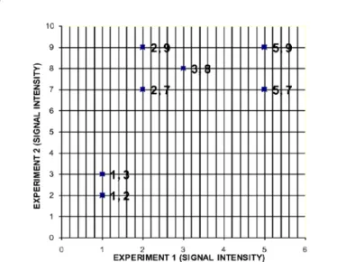
In table 1, experiment 1 expression values represent the X-axis, while experiment 2 represents the Y-axis, and each data point represents a gene. All the data points are plotted against each other using a scattered plot as in figure 2. However, if the third experiment is incorporated, it will form the Z-axis, and so on.

Results and Discussion

Task I: Choosing initial centroid at iteration 0

The algorithm starts at Iteration 0 with the initialization step of k-means. We make a guess of 3 clusters to be a good representative of the given expression data. Since 3 clusters are required i.e k=3, the first 3 data points with coordinates [(5,7), (3,8), (2,7)] forms the centre of the clusters to be formed. This is shown in red, green and yellow, respectively, as in table 2 and plotted in figure 3.

For simplicity, we choose our initial centroid (centre of a cluster of data points) based on the data sequence as each initial entry for the first three (3) data will form a centroid at first iteration 0. However, some authors choose initial centroid randomly, while other researchers engage in series of re-sampling. This is responsible for the problem of slight differences in results obtained as output by researchers at different runs of the k-means algorithm, using same data set and parameter k.

Task II: Computing for cluster membership using Euclidian

distance metric

Having identified the 3 centroids, it means that we have only

3 clusters, each of which the expression data can belong. Euclidian distance is calculated individually for all points to determine which point is closest to each of the 3 centroids.

For example: Euclidean distance for two 2D points, say:

Table 2: Coordinates of Centroids at Iteration 0. The centroid initially chosen,

are the first k number items, i.e. 1-3 from the ordered data set.

ITERATION 0

CENTROID 1 (Ct10)-Red CENTROID 2 (Ct20)-Blue CENTROID 3 (Ct30)-Yellow

X Y X Y X Y

5 7 3 8 2 7

Exp. 1 Exp. 2 Exp. 3 … Exp m-1 Exp m G1 0.5 2.9 2.1 … 3.5 2.3 G2 1.2 3.8 0.3 … 0.7 0.8 G3 1.5 2.6 1.0 … 1.1 2.6 G4 2.1 0.2 0.7 … 1.6 1.4 G5 0.7 4.5 2.1 … 2.8 3.3 … … … … … … … Gn-1 2.2 2.0 3.2 … 2.7 1.8 Gn 1.5 1.8 0.1 … 1.5 0.2

Figure 1: A simplified view of a typical microarray gene expression Matrix. Each experiment (Exp.1-Exp.m) represents a condition, while G1-Gn

represents each gene under study. To study each gene at all conditions, then analysis will be done from x, y, z …m as a coordinate.

GENES Experiment 1 Experiment 2

Gene 1 5 7 Gene 2 3 8 Gene 3 2 7 Gene 4 2 9 Gene 5 1 3 Gene 6 5 9 Gene 7 1 2

Table 1: Hypothetical Gene Expression data (Experiment 1 and Experiment 2). This is an example of 2×2 dimensional array containing two experiments carried out with seven genes.

Figure 2: Scattered graph of gene expression of hypothetical microarray data. The data layout is seen using this graph plot type. Experiment 1 is taken as the x-axis, while Experiment 2 is taken as the y axis.

( , )x y

P= P P and Q=( , )Q Qx y

Is given by _{( )}2 _{( )}2

x x y y

P Q− + P Q−

Where P is the centroid coordinate and Q represents coordinates of each gene data point.

If Centroid 1 Euclidean Distance at zero iteration=(Ct1ED₀) Centroid 2 Euclidean Distance at zero iteration=(Ct2ED₀) Centroid 3 Euclidean Distance at zero iteration=(Ct3ED₀) Then from table 2 above providing centroid coordinates: When Q= 5, 7 Ct1ED₀ =SQRT((5-5)2_+(7-7)2₎₌₀ Ct2ED₀=SQRT((3-5)2_+(8-7)2_)=2.24 Ct3ED₀=SQRT((2-5)2_+(7-7)2 _=3.00 When Q=3, 8 Ct1ED₀ =SQRT((5-3)2_+(7-8)2_)=2.24 Ct2ED₀=SQRT((3-3)2_+(8-8)2₎₌₀ Ct3ED₀=SQRT((2-3)2_+(7-8)2 _=1.41 When Q=2, 7 Ct1ED₀ =SQRT((5-2)2_+(7-7)2_)=3.00 Ct2ED₀=SQRT((3-2)2_+(8-7)2_)=1.41 Ct3ED₀=SQRT((2-2)2_+(7-7)2 ₌₀ When Q=2, 9 Ct1ED₀ =SQRT((5-2)2_+(7-9)2_)=3.61 Ct2ED₀=SQRT((3-2)2_+(8-9)2_)=1.41 Ct3ED₀=SQRT((2-2)2_+(7-9)2 _=2.00 When Q=1, 3 Ct1ED₀ =SQRT((5-1)2_+(7-3)2_)=5.66 Ct2ED₀=SQRT((3-1)2_+(8-3)2_)=5.39 Ct3ED₀=SQRT((2-1)2_+(7-3)2 _=4.12 When Q=5, 9 Ct1ED₀ =SQRT((5-5)2_+(7-9)2_)=2.00 Ct2ED₀=SQRT((3-5)2_+(8-9)2_)=2.20 Ct3ED₀=SQRT((2-5)2_+(7-9)2 _=3.61 When Q=1, 2 Ct1ED₀ =SQRT((5-1)2_+(7-2)2_)=6.40 Ct2ED₀=SQRT((3-1)2_+(8-2)2_)=6.32 Ct3ED₀=SQRT((2-1)2_+(7-2)2 _=5.10

At each value of Q above, we need to choose the smallest value among Ct1ED₀, Ct2ED₀ or Ct3ED₀. This is because we want to assign each gene expression data point (Q) to its closest cluster based on its minimum Euclidean distance, such that the choice of Ct1ED₀, Ct2ED₀ or Ct3ED₀ means that (5,7), for example belongs to one of Cluster 1(CLt1₀), Cluster 2(CLt2₀), or Cluster 3(CLt3₀), respectively at zero iteration.

However, the notation “Yes” value is used here in table 3 to denote the assignment of gene to a particular cluster that ‘win’ based on the smallest Euclidian distance, while “No” value for the centroid that ‘lost’ the assignment.

Task III: Taking decisions based on boolean variable

re-arrangement of gene-cluster assignment

Re-arranging the gene-cluster assignment of table 3 and

representing “Yes” with “1” and “No” with “0”, we have the following Boolean table below as in table 4.

The cluster to which each gene belongs is identified at this stage of iteration 0. It is necessary to compute the mean of coordinate for members of each cluster as in table 5.

The resultant mean of coordinates obtained will direct the next move to the current location of the new centroid. K-means performs a comparison check to determine if the previous mean coordinate of cluster is same with the current computed mean. If the same mean value is obtained such that all the centroid did not move, then the algorithm terminates, otherwise the algorithm move to iteration 1.

If Cluster 1: (5,7)

≠

≠

≠

Graphically, as the algorithm enters iteration 1 which is the second iteration, the centroid moves to their new coordinate position, as shown using guided arrow in figure 4.

Euclidean distance is again computed for iteration 1 (Table 7), using Euclidian distance formula as done for iteration 0 (table 3), using the values for the current centroid coordinates shown in table 6.

Transposing the last 3 columns in table 7 and re-arranging the gene-cluster assignment, such that any value representing “YES” is replaced with “1” and “NO” with “0”, we have the following boolean table in table 8. The observation is that only gene (2,7) was re-assigned from Cluster 3 (CLt3₁) to Cluster 2 (CLt2₁), as shown in table 8. Scanning horizontally on the rows of CLt1₁, CLt2₁ and CLt3₁ in table 8, revealed genes with values of “1” that belong to that cluster. These are captured under the “Remark” column. Genes 1, 6 belong to CLt1₁, Genes 2, 3, 4 belong to CLt2₁ and Genes 5, 7 belong to CLt3₁.

Based on this new re-assignment at the end of iteration 1, mean coordinates of cluster membership is re-computed as shown in table 9. As noted in earlier iterations, if the same mean value is obtained

Figure 3: Iteration 0 graph with designated centroids. The centroids 1-3 are now designated on the scattered graph with red, blue and yellow data points, respectively.

Genes 1 2 3 4 5 6 7 Decisions

Expressions (5,7) (3,8) (2,7) (2,9) (1,3) (5,9) (1,2)

CLt10 1 0 0 0 0 1 0 Genes (5,7);(5,9) belongs to Cluster 1

CLt20 0 1 0 1 0 0 0 Genes (3,8);(2,9) belongs to Cluster 2

CLt30 0 0 1 0 1 0 1 Genes (2,7);(1,3); (1,2) belongs to Cluster 3

Decisions were taken on membership of each cluster for the next iteration. Any intersection of a row representing either Cluster 1 (CLt10), Cluster 2 (CLt20 ) or Cluster 3

(CLt30)and gene columns (1-7). “0” indicate no cluster membership, while “1” indicates cluster membership.

Table 4: Boolean representation of gene-cluster assignment.

The mean position of new centriod position is being recomputed for the next iteration

Table 5: Computation of mean coordinate for cluster members.

CLUSTER 1 (CLt10)=YES CLUSTER 2 (CLt20)=YES CLUSTER 3 (CLt30)=YES

X-AXIS Y-AXIS X-AXIS Y-AXIS X-AXIS Y-AXIS

5 7 3 8 2 7

5 9 2 9 1 3

1 2

Mean Coordinate 5 8 2.5 8.5 1.3 4

The centroid position is now obtained from the re-computed mean coordinate in table 5

Table 6: Coordinates of centroids at iteration 1.

ITERATION 1

CENTROID 1 (Ct11)-Red CENTROID 2 (Ct21)-Blue CENTROID 3 (Ct31)-Yellow

X Y X Y X Y

5 8 2.5 8.5 1.3 4

At iteration1, Ct1ED1 means Centriod 1 Euclidean distances, Ct2ED1 means Centriod 2 Euclidean distances and Ct3ED1 means Centriod 3 Euclidean distances. CLt11

means Cluster 1 at Iteration 1, CLt21 means Cluster 2 at Iteration 1, CLt31 means Cluster 3 at Iteration 1. Here genes are assigned to clusters with a “YES” or “NO” value

Table 7: Euclidean distance and gene to cluster assignment for iteration 1.

ITERATION 1 EUCLIDIAN DISTANCES FOR CENTROIDS 1-3 GENE-CLUSTER ASSIGNMENT

X-AXIS Y-AXIS (Ct1ED1) (Ct2ED1) (Ct3ED1) (CLt11) (CLt21) (CLt31)

5 7 1 2.91548 4.737583 YES NO NO 3 8 2 0.70711 4.333346 NO YES NO 2 7 3.16228 1.58114 3.073189 NO YES NO 2 9 3.16228 0.70711 5.044253 NO YES NO 1 3 6.40312 5.70088 1.054082 NO NO YES 5 9 1 2.54951 6.200378 YES NO NO 1 2 7.2111 6.67083 2.027582 NO NO YES

In places where each cluster in the rows identified as CLt11, CLt21 and CLt31 contains the value of “1” gives the summary under “Remark”, as those genes to join that cluster.

Genes 1, 6 belong to CLt11, Genes 2,3,4 belong to CLt21 and Genes 5,7 belong to CLt31

Table 8: Boolean representation of gene-cluster assignment.

Genes 1 2 3 4 5 6 7

Remarks

Expressions (5,7) (3,8) (2,7) (2,9) (1,3) (5,9) (1,2)

CLt11 1 0 0 0 0 1 0 Genes 1 (5,7);6 (5,9) belongs to Cluster 1

CLt21 0 1 1 1 0 0 0 Genes 2 (3,8); 3 (2,7); 4 (2,9); belongs to Cluster 2

CLt31 0 0 0 0 1 0 1 Genes 5 (1,3); 7 (1,2) belongs to Cluster 3

At iteration 0, Ct1ED0 means Centriod 1 Euclidean distances, Ct2ED0 means Centriod 2 Euclidean distances and Ct3ED0 means Centriod 3 Euclidean distances. CLt10

means Cluster 1 at Iteration 0, CLt20 means Cluster 2 at Iteration 0, CLt30 means Cluster 3 at Iteration 1. Here genes are assigned to clusters with a “YES” or “NO” value.

Table 3: Euclidean Distance and gene to cluster assignment for iteration 0. ITERATION 0 Euclidean Distances Gene-Cluster Assignment

X-AXIS Y-AXIS (Ct1ED0) (Ct2ED0) (Ct3ED0) CLt10 CLt20 CL30

5 7 0 2.23607 3 YES NO NO 3 8 2.23607 0 1.414214 NO YES NO 2 7 3 1.41421 0 NO NO YES 2 9 3.60555 1.41421 2 NO YES NO 1 3 5.65685 5.38516 4.123106 NO NO YES 5 9 2 2.23607 3.605551 YES NO NO 1 2 6.40312 6.32456 5.09902 NO NO YES

such that all the centroids did not move, then the algorithm terminates, otherwise the algorithm move to iteration 1. Using our example to compare earlier mean coordinate with their corresponding current mean coordinate, we have:

Cluster 1: (5,8)=(5,8); Cluster 2: (2.5, 8.5)

≠

≠

It can be observed that only Cluster 1 did not move, while other mean coordinates moved. Therefore, the algorithm enters iteration 2, which is the third iteration as the centroid moves to their new coordinate position as shown in table 10.

Furthermore, guided arrows were used to specify the current re-computed mean coordinates as the new centroid locations in preparation for the next iteration. This is shown in figure 5.

Euclidean distance is again computed for iteration 2 (Table 11), using Euclidian distance formula as done in iteration 0 (Table 3 and 7), and also using the values for the current centroid coordinates, shown in table 10.

Performing Iteration 2 like other iteration steps and generating Euclidian Distance table as in table 11, Boolean representation of gene-cluster assignment was also similarly created as in table 12. Mean The averages of the coordinate are the re-computed centroid 1-3 locations on the scattered graph

Table 10: Coordinates of centroids at iteration 2.

ITERATION 2

CENTROID 1 (Ct12)-Red CENTROID 2 (Ct22)-Blue CENTROID 3 (Ct32)-Yellow

X Y X Y X Y

5 8 2.3 8 1 1.5

At iteration2, Ct1ED2 means Centriod 1 Euclidean distances, Ct2ED2 means Centriod 2 Euclidean distances and Ct3ED2 means Centriod 3 Euclidean distances. CLt12

means Cluster 1 at Iteration 2, CLt22 means Cluster 2 at Iteration 2, CLt32 means Cluster 3 at Iteration 2. Here genes are assigned to clusters with a “YES” or “NO” value

Table 11: Euclidean distance and gene to cluster assignment for iteration 2. ITERATION 2 EUCLIDEAN DISTANCES GENE-CLUSTER ASSIGNMENT

X-AXIS Y-AXIS (Ct1ED2) (Ct2ED2) (Ct3ED2) (CLt12) (CLt22) (CLt32)

5 7 1 2.84803 6.020797 YES NO NO 3 8 2 0.6667 5.85235 NO YES NO 2 7 3.16228 1.05408 4.609772 NO YES NO 2 9 3.16228 1.05408 6.576473 NO YES NO 1 3 6.40312 5.17472 0.5 NO NO YES 5 9 1 2.84803 7.632169 YES NO NO 1 2 7.2111 6.14636 0.5 NO NO YES

In places where each cluster in the rows identified as CLt12, CLt22 and CLt32 contains the value of “1” gives the summary under “Remark” as those genes to join that cluster.

Genes 1, 6 belong to CLt12, Genes 2,3, 4 belong to CLt22 and Genes 5, 7 belong to CLt32

Table 12: Boolean representation of gene-cluster assignment.

Genes 1 2 3 4 5 6 7 Remarks

Expressions (5,7) (3,8) (2,7) (2,9) (1,3) (5,9) (1,2)

CLt12 1 0 0 0 0 1 0 Genes (5,7);(5,9) belongs to Cluster 1

CLt22 0 1 1 1 0 0 0 Genes(3,8); (2,7); (2,9); belongs to Cluster 2

CLt32 0 0 0 0 1 0 1 Genes (1,3); (1,2) belongs to Cluster 3

Mean coordinates are re-computed to determine if current centroid position has shifted from previous position

Table 13: Computation of mean coordinate for cluster members at the end of iteration 2.

ITERATION 2

CENTROID 1 (Ct11)-Red CENTROID 2 (Ct21)-Blue CENTROID 3 (Ct31)-Yellow

X Y X Y X Y 5 7 3 8 1 3 5 9 2 7 1 2 2 9 Mean Coordinate 5 8 2.3 8 1 1.5 ITERATION 1

CENTROID 1 (Ct11)-Red CENTROID 2 (Ct21)-Blue CENTROID 3 (Ct31)-Yellow

X Y X Y X Y

5 7 3 8 1 3

5 9 2 7 1 2

2 9

Mean Coordinate 5 8 2.3 8 1 1.5

The averages of each coordinate are re-computed separately to obtain a new mean coordinate

Coordinates of Cluster was computed for iteration 2, it is however observed that all the mean coordinates of Iteration 1 remained unchanged at Iteration 2.

Invariably, cluster membership remain the same from the last iteration 1, meaning that no individual data point shifted from one cluster to the other at the end of iteration 2 (Table 13). This shows that convergence point has been reached and the algorithm terminates at Iteration 2. This therefore terminates the algorithm, successfully indicating that cluster 1 has 2 data points clustered together, cluster 2 has 3 data points clustered together and cluster 3 has 2 data points clustered together. Figure 6 precisely shows the gene members of the final clusters identifying the specific cluster they belong.

Conclusion

From the foregoing, we can define k-means clustering as an algorithm used to group objects or data points into user-defined number

of classes called clusters based on certain attributes, whereby each data point presented is allocated to a cluster, whose centroid maintains the shortest distance to that data point. The k-means algorithm does not necessarily provide a global optimum, and depending on the starting values used, the algorithm terminates at a local optimum that is never verifiably globally optimal [20]. There could be numerous local optima for a data set, the choice of starting values for the k-means algorithm is all the more crucial, and several alternatives have been proposed in an attempt to avoid locally optimal solutions. It is suggested that local optima, can be avoided by performing the k-means method several times, with different starting values, accepting the best solution with less standard error. However, the method of different starting values is clumpsy, and will not permit ease of quick and rough comparison of k-means cluster membership. Interestingly, there are three possible ways to select your initial centroids: first k instances, random sampling or random partition. In all, data are assigned to their nearest centroid and new k centroids are computed for the next iteration iteratively, till convergence is reached. It is due to the clumsy nature of using different starting that we propose a specific use of k initial data points, as centroid for the different runs of k-means.

Our laboratory developed a C++ and MATLAB-based Metric Matrices k-means (MMk-means) clustering algorithm [1,29], to cluster genes to their functional roles with a view of obtaining further knowledge on many P. falciparum genes [33]. We now successfully follow this recent algorithm development with a demonstration and analysis of the operational and iterative mechanism of k-means clustering. A Step-by-step k-means walk approachwas applied using a simplified view of high throughput microarray data as a test case. This will help to provide a better knowledge of the computational framework of the k-means algorithms and its variants, as commonly applied by biologists and bioinformaticians. Interestingly, only two columns depicting two experimental conditions of microarray data has been used for various graphic-centric tasks for purpose of clarity, the result outcome as discussed in this work is unique in its simplicity, this is because the display of an entire microarray data Figure 4: Iteration 1 graph with designated centroid shift to new location.

The arrow specifies the shift in position of centroids.

Figure 5: K-mean iteration 2 plot showing centroid movement. Ct11 (Centroid 1 at 1st iteration) move to Ct12 (Centroid 1 at 2nd iteration)

Ct21 (Centroid 2 at 1st iteration) move to Ct22 (Centroid 2 at 2nd iteration)

Ct31 (Centroid 3 at 1st iteration) move to Ct32 (Centroid 3 at 2nd iteration)

Figure 6: Iteration 2 plot showing convergence & final clusters.

Ct11 (Centroid 1 at 1st iteration) move to Ct12 (Centroid 1 at 2nd iteration)

Ct21 (Centroid 2 at 1st iteration) move to Ct22 (Centroid 2 at 2nd iteration)

points will be too cluttered and more clumsy to show concisely. It is imperative to state that if the number of genes and dimension of the data concerned is large, the same process occurs but it is likely that the number of iterations will also be large. With good understanding of k-means operational mechanisms, investigators may need clever ways of obtaining desired result through flexibility in design and its application. In addition, this paper serves as an invaluable resource for algorithm designers, programmers and investigators that requires the application of k-means clustering in their work.

References

1. Osamor VC, Adebiyi EF, Oyelade JO, Doumbia S (2012) Reducing the time requirement of k-means algorithm. PLoS One 7: e49946.

2. Yona G, Dirks W, Rahman S (2009) Comparing algorithms for clustering of expression data: how to assess gene clusters. Methods Mol Biol 541: 479-509. 3. Osamor VC (2009) Experimental and computational applications of microarray

technology for malaria eradication in africa. Scientific Research and Essays4: 652-664.

4. Breman JG, Egan A, Keusch GT (2001) The intolerable burden of malaria: a new look at the numbers. Am J Trop Med Hyg 64: iv-vii.

5. Le Roch KG, Zhou Y, Batalov S, Winzeler EA (2002) Monitoring the chromosome 2 intraerythrocytic transcriptome of Plasmodium falciparum using oligonucleotide arrays. Am J Trop Med Hyg 67: 233-243.

6. Le Roch KG, Zhou Y, Blair PL, Grainger M, Moch JK, et al. (2003) Discovery of

gene function by expression profiling of the malaria parasite life cycle. Science

301: 1503-1508.

7. Hayward RE, Derisi JL, Alfadhli S, Kaslow DC, Brown PO, et al. (2000)

Shotgun DNA microarrays and stage-specific gene expression in Plasmodium falciparum malaria. Mol Microbiol 35: 6-14.

8. Bozdech Z, Llinás M, Pulliam BL, Wong ED, Zhu J, et al. (2003) The transcriptome of the intraerythrocytic developmental cycle of Plasmodium falciparum. PLoS Biol 1: E5

9. Bozdech Z, Zhu J, Joachimiak MP, Cohen FE, Pulliam B, et al. (2003)

Expression profiling of the schizont and trophozoite stages of Plasmodium falciparum with a long-oligonucleotide micrarray. Genome Biol 4: R9. 10. Daily JP, Le Roch KG, Sarr O, Fang X, Zhou Y, et al. (2004) In vivo transcriptional

profiling of Plasmodium falciparum. Malar J 3: 30.

11. Daily JP, Scanfeld D, Pochet N, Le Roch K, Plouffe D, et al. (2007) Distinct physiological states of Plasmodium falciparum in malaria-infected patients. Nature 450: 1091-1095.

12. Llinás M, Bozdech Z, Wong ED, Adai AT, DeRisi JL (2006) Comparative whole genome transcriptome analysis of three Plasmodium falciparum strains. Nucleic Acids Res 34: 1166-1173.

13. Tarun AS, Peng X, Dumpit RF, Ogata Y, Silva-Rivera H, et al. (2008) A combined transcriptome and proteome survey of malaria parasite liver stages. Proc Natl Acad Sci U S A 105: 305-310.

14. Kissinger JC, Brunk BP, Crabtree J, Fraunholz MJ, Gajria B, et al. (2002) The

Plasmodium genome database. Nature 419: 490-492.

15. Bahl A, Brunk B, Crabtree J, Fraunholz MJ, Gajria B, et al. (2003) PlasmoDB: the Plasmodium genome resource. A database integrating experimental and computational data. Nucleic Acids Res 31: 212-215.

16. Clements FE (1954) Use of cluster analysis with anthropological data. Am Anthropol 56: 180-199.

17. Sneath PH (1957) The application of computers to taxonomy. J Gen Microbiol 17: 201-226.

18. Sokal RR, Michener CD (1958) A statistical method for evaluating systematic relationships (Vol 38). University of Kansas, Kansas.

19. Lloyd SP (1957) Least squares quantization in PCM. IEEE Trans Inf Theory 28: 129-137.

20. MacQueen J (1967) Some methods for classification and analysis of multi-variate observations. In: Proceedings of the fifth Berkeley Symposium on

mathematical statistics and probability, LeCam LM, Neyman J (eds). University of California Press, Berkeley.

21. Heyer LJ, Kruglyak S, Yooseph S (1999) Exploring expression data:

identification and analysis of coexpressed genes. Genome Res 9: 1106-1115.

22. Tamayo P, Slonim D, Mesirov J, Zhu Q, Kitareewan S, et al. (1999) Interpreting patterns of gene expression with self-organizing maps: methods and application to hematopoietic differentiation. Proc Natl Acad Sci U S A 96: 2907-2912. 23. Pelleg D, Moore A (2000) X-means: Extending K-means with efficient estimation

of the number of clusters. In: Proceedings of the Seventeenth International Conference on Machine Learning. Morgan Kaufmann, San Francisco. 24. Hamerly G, Elkan C (2003) Learning the k in k-means. In: proceedings of the

seventeenth annual conference on neural information processing systems (NIPS).

25. Feng Y, Hamerly G (2006) PG-means: learning the number of clusters in data. In:Proceedings of the twentieth annual conference on neural information processing systems (NIPS).

26. Fahim AM, Salem AM, Torkey FA, Ramadan MA (2006) An efficient enhanced

k-means clustering algorithm.Journal of Zhejiang UniversitySCIENCE A 7: 1626-1633.

27. Wicker N, Dembele D, Raffelsberger W, Poch O (2002) Density of points clustering, application to transcriptomic data analysis. Nucleic Acids Res 30: 3992-4000.

28. Dembélé D, Kastner P (2003) Fuzzy C-means method for clustering microarray data. Bioinformatics 19: 973-980.

29. Osamor VC (2010) Simultaneous and Single Gene Expression: Computational Analysis for Malaria Treatment Discovery. VDM Publishing, Saarbruken. 30. Kanungo T, Mount DM, Netanyahu NS, Piatko CD, Silverman R, et al. (2004)

A local search approximation algorithm for k-means comput geom 28: 89-112. 31. Teknomo K (2006) K-means clustering tutorials.

32. Sammy L (2012) k-Means clustering & finding k.

33. Osamor VC, Adebiyi E, Doumbia S (2010) Clustering Plasmodium falciparum

genes to their functional roles using k-means. IACSIT Int J Eng Technol 2: 215-225.

Citation: Osamor VC, Adebiyi EF, Enekwa EH (2013) k-Means Walk: Unveiling Operational Mechanism of a Popular Clustering Approach for Microarray Data. J Comput Sci Syst Biol 6: 035-042. doi:10.4172/jcsb.1000098

Submit your next manuscript and get advantages of OMICS Group submissions

Unique features:

• User friendly/feasible website-translation of your paper to 50 world’s leading languages • Audio Version of published paper

• Digital articles to share and explore

Special features:

• 250 Open Access Journals • 20,000 editorial team • 21 days rapid review process

• Quality and quick editorial, review and publication processing

• Indexing at PubMed (partial), Scopus, DOAJ, EBSCO, Index Copernicus and Google Scholar etc • Sharing Option: Social Networking Enabled

• Authors, Reviewers and Editors rewarded with online Scientific Credits • Better discount for your subsequent articles