Author: Daniel Monzon´ıs Laparra
Facultat de F´ısica, Universitat de Barcelona, Diagonal 645, 08028 Barcelona, Spain. Advisor: Tristan Cantat-Gaudin
Abstract: The aim of this work is to study several open clusters previously identified in other studies, but using the newer and more precise data from the Gaia DR2 catalogue, trying to verify their existence and use the photometry included in the catalogue to estimate their age and the total interstellar extinction.
I. INTRODUCTION
Open clusters are groups of stars formed from the same molecular cloud simultaneously, and therefore the stars in the cluster share many properties like age, position, proper motion and composition. Because of this, many of these properties can be estimated much more easily from a cluster than from a single star. This information can then be used to trace the structure of the Milky Way, and makes open clusters very interesting for studying stellar evolution and stellar structure, since the only parameter that varies is the mass of each star.
Over 1200 open clusters have been identified within the Milky Way, but it is thought that there exist around 105 open clusters in the galaxy, since most open clusters form near the galactic plane, where the interstellar extinction is higher due to the higher amount of dust, making their observation much harder [3].
With the new release of data from Gaia, we can study open clusters with more precision than ever before. This data includes positions in the sky, proper motions, par-allaxes, and magnitudes in three different photometric filters for over 1 billion stars.
Using the data from the UCAC4 catalogue, Sampedro et al. reported the existence of 1876 open clusters, using three different membership methods [1]. With the release of the Gaia DR2 catalogue, which contains more precise astrometric data, it is now possible to find and verify the existence of clusters more accurately. There have already been attempts to identify open clusters using the Gaia DR2 catalogue, for instance, in the study of Cantat-Gaudin et al., 1229 clusters were identified with the new data [2].
As a first step, we will crossmatch the data from both studies to find the clusters that haven’t already been ver-ified. We will then use the data from Gaia to find some cases from the list which are clearly clusters. Finally, we will estimate the age and total interstellar extinction of these clusters.
II. THE GAIA DR2 CATALOGUE
The second release of data from Gaia, in the form of the Gaia DR2 catalogue, introduces high-precision measure-ments of various astrometry parameters, like proper
mo-tions and parallaxes, as well as photometric information for about 1.7 billion sources [4]. The catalogue contains a 5-parameter astrometric solution for over 1.3 billion stars, which include the position in the sky given by the right ascension and declination, the proper motion and the parallax. For the rest of the stars, which are the very faint ones (G >21), a 2-parameter astrometric solution is given instead, with only the positions in the sky.
For bright stars (G <15) the uncertainty in the posi-tions and parallax is about 0.02−0.04 mas, and the un-certainty in the proper motions is about 0.07 mas yr−1. We will only be working with stars of at mostG= 17, for which the uncertainty in the positions and parallax is of 0.1 mas and of 0.2 mas yr−1 in the proper motions. Fig-ure 1 illustrates the improvement in precision of the as-trometric parameters, by comparing the proper motions of a well known cluster with the data from the PPMXL catalogue [5] and Gaia DR2.
The catalogue also lists valuable information on the photometry of most of its sources on the G, GBP and
GRP photometric passbands.
III. IDENTIFYING OPEN CLUSTERS As a first measure to reduce the number of clusters that need to be verified, we will only check the clusters whose name is not present in the data from both studies. By applying said filter, we end up with a list of 890 clusters, which more than the 647 we expected, due mainly to naming inconsistencies and possibly to one study having found some clusters that the other has not. However, our main focus will be the 647 clusters that Sampedro found with the less precise data from UCAC4.
For each of these 890 clusters, we compute the mean right ascensionαand declinationδ, which we will use as the center point of a circle with radius max(δ)−min(δ)
2 ,
where we consider the set of declinations of the stars in each cluster. Then, we query the data from the Gaia DR2 catalogue for the region encompassed by this circle. We get stars with a magnitude G < 17, since the data from the UCAC4 catalogue does not show stars fainter than G ≈ 17. This gives us the data for all the stars in the queried region, so we crossmatch this data with the data from the original study to leave only the stars
FIG. 1: Comparison of the data from PPMXL and Gaia DR2 for the proper motions of the cluster Ivanov 2 [6]. We can see that the proper motions also look more compact with the data from Gaia, confirming that it is in fact an open cluster.
that are listed in Sampedro’s study as being part of the cluster.
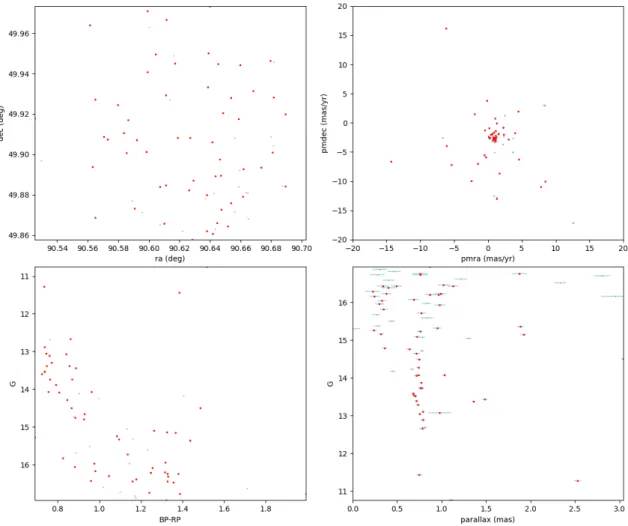
Figure 2 shows one example of the plots that were made for each of the clusters, for the case of NGC 2126, which will be studied in the next section. Note that, in this case, the proper motion space is pretty compact, showing that the stars are moving together, and there is a clear straight line in the parallax versus magnitude plot, showing that the stars are at the same distance. Note that if we just look at the position plot of the stars, it is not clear that it is in fact a cluster, as it does not appear as a compact overdensity. However, looking at the proper motion and parallax plots, it becomes clear that the stars are moving together and are at the same distance, confirming that this is in fact a cluster. In the color-magnitude diagram, we can see that some stars have already left the main sequence. We will study this in more detail in the following section.
To filter out the repeated cases due to name inconsis-tencies, the cluster positions from the study of Cantat-Gaudin were also added to the plots, so in the case of a repeated cluster, we would see it near the center in the position plot, which corresponds to the first plot as shown in Figure 2.
After examining the plots for all 890 clusters, excluding repetitions, we found that only 14 of them were really compact in proper motion, leading us to believe that the rest of them probably are not actually clusters. These 14 cases confirmed to be clusters are studied further in the next section.
IV. ESTIMATING THE AGE AND INTERSTELLAR EXTINCTION OF THE
CLUSTER
In this section we discuss the procedure followed to estimate the age and interstellar extinction of some clus-ters. We applied this method to a total of 14 clusters, some of which are taken from the list of verified clusters in the study of Cantat-Gaudin, and the rest are cases from the study of Sampedro which we have verified in the previous section. The complete list of investigated clusters is given in Table I, along with some parameters. To obtain the list of probable members, the UPMASK classification method [2] was applied. Note that a lower parallax means a greater distance.
Cluster Position (deg) Parallax (mas) Members
Alessi 3 (109.95,−46.05) 3.5619 243 Berkeley 100 (351.48,63.78) 0.1461 57 Collinder 421 (305.83,41.69) 0.8169 283 ESO 332 08 (253.80,−40.96) 0.5332 417 Herschel 1 (116.72,0.15) 3.3385 149 NGC 752 (29.24,37.77) 2.2245 263 NGC 1039 (40.51,42.74) 1.9350 659 NGC 2126 (90.65,49.91) 0.7490 151 NGC 2169 (92.12,13.94) 0.9863 133 NGC 2287 (101.51,−20.70) 1.3503 673 NGC 2360 (109.44,−15.63) 0.8994 695 NGC 2479 (118.76,−17.73) 0.6311 159 Ruprecth 8 (105.41,−13.56) 0.4278 138 Stock 6 (35.93,63.79) 0.9536 144
TABLE I: List of clusters that have been studied, includ-ing their mean position (given in (α,δ)) and mean parallax, computed using the data from Gaia DR2, and the number of member stars of the cluster.
To determine the age and interstellar extinction of the clusters, we make use of the theoretical stellar evolution model. Stars enter the main sequence soon after their birth, where they stay most of their life burning hydro-gen. When their hydrogen cores deplete, they leave the main sequence and start burning the helium in their core resulting from the fusion of hydrogen atoms. When this happens, the stars maintain a similar brightness, but be-come much redder in color. The brighter a star is, the faster it will burn through its hydrogen core and leave the main sequence.
If we represent the stars in an open cluster in a colour-magnitude diagram (CMD), one can see the brightness at which the stars are starting to leave the main sequence.
FIG. 2: Data from the candidate cluster NGC 2126. The red dots correspond to stars from the Gaia DR2 catalogue that match a star from Sampedro’s study. Top left: Plot of the star positions; Top right: Plot of the proper motions; Bottom left: Colour-magnitude diagram; Bottom right: Plot of the parallax against the total magnitude, where we can see a straight vertical line showing that the stars are at the same distance.
This is called the turnoff point, and it can be used to estimate the age of the cluster.
To be able to represent the data from Gaia in a CMD, we need to shift from apparent to absolute magnitude, and we also need to take into account the interstellar extinction, which makes the stars appear redder and less bright than what they actually are.
LetM be the absolute magnitude, andmthe apparent magnitude without any corrections due to the interstellar reddening. Then, we define the distance modulus asµ= m−M. Since we don’t have the absolute magnitude, we need to relate this to the distance of the stars in the cluster, which is given by the parallax.
Remember that
m=−2.5 log10
F(d)
F0
where F is the observed flux density of the star, and F0 is the reference flux. The absolute magnitude M is the apparent magnitude of the star if it was placed at a distance of 10 parsecs. The fluxF and luminosityLof a
star are related by the distance to the stardby
F = L 4πd2
and since the luminosity is an intrinsic property of a star, we find the relation
F1 F2 = d 2 d1 2 (1)
Then, using this relation in the expression m−M =
−2.5 log10F(Fd(=10)d) , one can rewrite the distance mod-ulus in terms of the distance as
µ=m−M = 5 log10
d
10
(2)
where d is in parsecs. We can use equation 2 with the data from Gaia, since the relation between the parallax pgiven in arcseconds and the distancedgiven in parsecs is justd=p−1.
Given that the stars in an open cluster are relatively close together, we shift every star in the plot by the dis-tance modulus of the mean parallax of the cluster. We chose this approach instead of using shifting each star by its individual distance modulus because for more distant stars the error in the parallax is higher, so there might be a lot of discrepancy between the parallaxes of some of the stars in the cluster and the CMD would be less clear. Another option would have been to treat the dis-tance modulus as a third free parameter to estimate via isochrone fitting, which would also avoid this problem but would make the process harder.
An isochrone is the line that would be drawn in a CMD if we varied the mass of the star at a fixed age. Since the stars in an open cluster have the same age, we can find an isochrone that fits the CMD of the stars in the cluster to determine its age. The isochrones used are from PAR-SEC [7], with the photometric system from Gaia DR2, and including the interstellar extinctionAV on a
star-to-star basis [8]. The metallicity of the star-to-stars, which mea-sures the abundance of heavy elements, is also included in the isochrones used, with a value ofZ= 0.0152, which is the metallicity of the Sun. An example of the result of fitting an isochrone to the cluster data can be seen in Figure 3.
FIG. 3: CMD of the cluster NGC 752, with an isochrone of age 1.78Gyr and AV = 0.1, with a shift in total magnitude
given by the mean distance modulus ¯µ= 8.264.
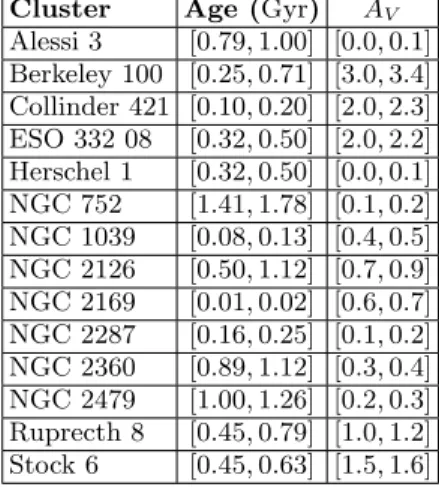
The estimated ages and interstellar extinctionAV for
all the clusters studied is shown in Table II.
Cluster Age (Gyr) AV
Alessi 3 [0.79,1.00] [0.0,0.1] Berkeley 100 [0.25,0.71] [3.0,3.4] Collinder 421 [0.10,0.20] [2.0,2.3] ESO 332 08 [0.32,0.50] [2.0,2.2] Herschel 1 [0.32,0.50] [0.0,0.1] NGC 752 [1.41,1.78] [0.1,0.2] NGC 1039 [0.08,0.13] [0.4,0.5] NGC 2126 [0.50,1.12] [0.7,0.9] NGC 2169 [0.01,0.02] [0.6,0.7] NGC 2287 [0.16,0.25] [0.1,0.2] NGC 2360 [0.89,1.12] [0.3,0.4] NGC 2479 [1.00,1.26] [0.2,0.3] Ruprecth 8 [0.45,0.79] [1.0,1.2] Stock 6 [0.45,0.63] [1.5,1.6]
TABLE II: Estimated ages and interstellar extinctionAV for
the clusters studied via isochrone fitting, given in ranges.
V. ISSUES WHEN FITTING ISOCHRONES A. Unresolved binary stars
Many stellar systems are binary stars, systems formed by two stars orbiting each other. If they are distant, some these systems may be unresolved and seen as a single object. In a CMD, unresolved binary stars would appear as a secondary line in the main sequence which is brighter than the rest. A clear example of this can be seen in Figure 3. This can make the main sequence line in the CMD appear wider than it actually is, and can be a problem when fitting isochrones.
To avoid this problem, when we find a wide main se-quence line, we try to fit the isochrone near the less lu-minous stars, which should be single star systems.
B. Differential extinction
In this work, the reddening due to the interstellar extinction had a fixed value and was included in the isochrones used to estimate the parameters of the clus-ters. However, in some cases, like for instance Stock 6, the extinction is not the same for all stars in the clus-ter. In the case of Stock 6, more distant stars appeared to have significantly more extinction, and this makes the stars appear more scattered in the CMD, making the fit-ting harder. To avoid this problem, we would have to estimate the extinction for each star individually, and apply the corrections on each of the stars, instead of ap-plying a global extinction for all the stars in the cluster.
C. Blue stragglers
Blue stragglers are stars in open clusters that appear to be brighter and bluer than the stars at the turnoff point in the CMD. They can make the turnoff point unclear,
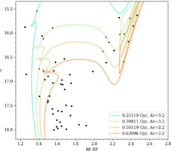
especially if we also have other effects which make the plots less clear, like the ones discussed previously. In Figure 4 we can see some stars which are likely to be blue stragglers, and add uncertainty to the location of the turnoff point.
FIG. 4: CMD of the cluster Berkeley 100 with various
isochrones, and AV = 3.2, with a shift in total magnitude
given by the mean distance modulus ¯µ= 14.177.
The reason as to why blue stragglers exist is still not well known, but one plausible theory is that they are formed from binary stars, in which one of the stars merges with the other by transferring its mass [9].
VI. CONCLUSIONS
We have identified various open clusters listed in other studies, using the more recent and precise data from the Gaia DR2 catalogue. For some of these clusters, we have also estimated their ages and total interstellar extinction, while explaining in detail the methodology followed to do
so, using the isochrones made from the theoretical models of stellar evolution.
Distant clusters have generally been harder to study for various reasons, mainly due to the error in the astromet-ric and photometastromet-ric parameters. However, these errors are still much lower than what we had before, so the Gaia data has allowed us to characterise them in greater detail. This will allow future works to study many open clusters for which there was not precise enough data before, and to further our understanding of the stellar content of the galaxy.
VII. APPENDIX
Throughout this work, we mention the interstellar ex-tinction and its reddening effect without getting into the details of what it is. Interstellar extinction is an effect produced by dust clouds, which absorb and scatter light. This extinction, however, is selective, meaning that light of different wavelengths is affected differently. In gen-eral, extinction is stronger at shorter wavelengths, which causes a reddening of the light. We can define the total extinction at a certain wavelength λ, Aλ, by adding a
term in equation 2, mλ−Mλ= 5 log10 d 10 +Aλ (3)
which is defined as the total extinction for the visual photometric band V, AV. The reddening effect due to
the extinction is then defined as
EB−V =AB−AV (4)
Acknowledgments
I would like to thank my advisor Tristan Cantat-Gaudin, who guided me through the process of this work and provided very useful knowledge. I would also like to thank Miriam for her support during all these years.
[1] L. Sampedro, W. S. Dias, E. J. Alfaro, H. Monteiro, and A. Molino, (2017), arXiv:1706.05581 [astro-ph.SR]. [2] T. Cantat-Gaudin, C. Jordi, A. Vallenari, et al., (2018),
arXiv:1805.08726 [astro-ph.GA]
[3] K. Janes,Star Clusters, Encyclopedia of Astronomy and Astrophysics, (Nature Publishing Group, 2001)
[4] A.G.A. Brown, A. Vallenari, T. Prusti et al., (2018), arXiv:1804.09365 [astro-ph.GA]
[5] S. Roeser, M. Demleitner and E. Schilbach, (2010), arXiv:1003.5852 [astro-ph.GA]
[6] A. L. Tadross, R. Bendary, (2014), arXiv:1403.3014 [astro-ph.GA]
[7] A. Bressan, P. Marigo, L. Girardi, B. Salasnich, C. Dal Cero, S. Rubele, and A. Nanni, (2012), arXiv:1208.4498 [astro-ph.SR]
[8] L. Girardi, J. Dalcanton, B. Williams, et al., (2008), arXiv:0804.0498 [astro-ph]
[9] Aaron M. Geller, Robert D. Mathieu, (2011),
![FIG. 1: Comparison of the data from PPMXL and Gaia DR2 for the proper motions of the cluster Ivanov 2 [6]](https://thumb-us.123doks.com/thumbv2/123dok_us/25146.3003941/2.892.126.403.78.553/fig-comparison-ppmxl-gaia-proper-motions-cluster-ivanov.webp)