Bayesian Semiparametric Stochastic Volatility Modeling

(1)

WP 23-09

Mark J. Jensen

Federal Reserve Bank of Atlanta, USA

John M. Maheu

University of Toronto, Canada

and

The Rimini Centre for Economic Analysis, Italy

BAYESIAN SEMIPARAMETRIC

STOCHASTIC VOLATILITY MODELING

Copyright belongs to the author. Small sections of the text, not exceeding three paragraphs, can be used provided proper acknowledgement is given.

The Rimini Centre for Economic Analysis (RCEA) was established in March 2007. RCEA is a private, non-profit organization dedicated to independent research in Applied and Theoretical Economics and related fields. RCEA organizes seminars and workshops, sponsors a general interest journal The Review of Economic Analysis, and organizes a biennial conference: Small Open Economies in the Globalized World

(SOEGW). Scientific work contributed by the RCEA Scholars is published in the RCEA Working Papers series.

The views expressed in this paper are those of the authors. No responsibility for them should be attributed to the Rimini Centre for Economic Analysis.

The Rimini Centre for Economic Analysis

(2)

Bayesian semiparametric stochastic volatility modeling

∗

Mark J. Jensen John M. Maheu

Federal Reserve Bank of Atlanta University of Toronto and RCEA

[email protected] [email protected]

June 2009

Abstract: This paper extends the existing fully parametric Bayesian literature on stochastic volatility to allow for more general return distributions. Instead of specifying a particular distribution for the return innovation, nonparametric Bayesian methods are used to ﬂexibly model the skewness and kurtosis of the distribution while the dynamics of volatility continue to be modeled with a parametric structure. Our semiparametric Bayesian approach provides a full characterization of parametric and distributional uncertainty. A Markov chain Monte Carlo sampling approach to estimation is presented with theoretical and computational issues for simulation from the posterior predictive distributions. An empirical example compares the new model to standard parametric stochastic volatility models.

∗_{We would like to thank the seminar participants at the 24th Canadian Econometric Study Group}

Con-ference held in Montreal, the 7th All-Georgia ConCon-ference held at the Federal Reserve Bank of Atlanta, the RCEA conference on Econometrics 2007, held in Rimini, Italy, the 15th Annual Symposium of the Society for Nonlinear Dynamics and Econometrics held at the Federal Reserve Bank of San Francisco, the 2009 Seminar on Bayesian Inference in Econometrics and Statistics held at Washington University in Saint Louis, and the Department of Economics at New York University and Oregon State University. In addition, we express our appreciation for the comments and suggestions from John Geweke, Thanasis Stengos and George Tauchen. Maheu is grateful to the SSHRC for ﬁnancial support. The views expressed here are ours and not necessarily those of the Federal Reserve Bank of Atlanta or the Federal Reserve System.

(3)

1 Introduction

This paper proposes a model of asset returns that draws from the existing literature on autoregressive stochastic volatility (SV) models and the advances made in Bayesian non-parametric modeling and sampling to create a seminon-parametric SV model. By applying both parametric and nonparametric features to the return process, an estimable SV model with a flexible nonparametric innovation distribution is provided. The nonparametric portion of the model consists of an infinitely ordered mixture of normals whose component probabil-ities and parameters are modeled with a particular Bayesian prior - the Dirichlet process mixture prior (DPM). Under the DPM representation of the returns conditional distribu-tion, our model produces a more robust predictive density of returns than parametric SV models. The paper takes a likelihood based approach to model inference and provides exact finite sample properties, including a full characterization of parametric and distributional uncertainty.

There exists a long history of modeling asset returns with a mixture of normals (see Press (1967); Praetz (1972); Clark (1973); Gonedes (1974); Kon (1984)). These early mixture models produced fat-tailed behavior but could not capture the dynamic clustering observed in the conditional variance of returns. SV models were designed to ﬁt this time-varying behavior (see Taylor (1986); Harvey et al. (1994)). They consist of a continuous mixture of normals where their variances follow a dynamic stochastic process. However, parametric SV models have not fully captured the asymmetries and leptokurtotic behavior present in return data (see Gallant et al. (1997); Mahieu & Schotman (1998); Liesenfeld & Jung (2000); Meddahi (2001); and Durham (2006)). These characteristics play an important role in the pricing of derivatives, the measuring and managing of risk, and in portfolio selection. A ﬂexible nonparametric version of the SV model will be useful to risk and portfolio managers alike.

The DPM consists of modeling the probabilities and parameters of an inﬁnitely ordered mixture model with the Dirichlet process prior of Ferguson (1973). As a Bayesian nonpara-metric estimator of a unknown distribution, the DPM oﬀers a number of attractive features;

i) the DPM spans the class of continuous distributions (Escobar & West (1995) and Ghosal et al. (1999)), ii) the DPM is more ﬂexible and realistic than a mixture model with a prede-termined number of components,iii) the Dirichlet process prior helps determine the number of mixture clusters that best ﬁts the data, iv) as an almost surely discrete prior it is parsi-monous, v) as a conjugate prior it is easy to use and facilitates Gibbs sampling, and vi) it works well in practice.1

1_{Examples of the DPM being used in economics include Chib & Hamilton (2002), Conley et al. (2008),}

Griﬃn & Steel (2004), Hirano (2002), Jensen (2004), Kacperczyk et al. (2005), and Tiwari et al. (1988). Jensen (2004) uses a DPM to model the distribution of additive noise of log-squared returns while in this paper we are concerned with the conditional distribution of returns.

(4)

This paper provides a flexible semiparametric stochastic volatility, Dirichlet process mix-ture model (SV-DPM) by combining a nonparametric independently identically distributed DPM model of innovations scaled by a autoregressive model of the return’s latent conditional variance process.2 The SV-DPM will nest within it parametric versions of the SV model. A Markov chain Monte Carlo (MCMC) sampler is constructed to estimate the unknown pa-rameters of the SV-DPM. Our MCMC algorithm extends the DPM samplers of West et al. (1994) and MacEachern & Müller (1998) to the time-varying structure of the SV model. Due to the independence between the volatility process and the DPM, a tractable efficient posterior sampler is possible. Conditional on the value of the other unknowns, one block of our sampler consists of drawing the parameters of the clusters, while the other blocks draw the parameters and volatilities for the SV model’s latent volatility process (see Chib et al. (2002); Eraker et al. (2003); Jacquier et al. (1994 2004); and Kim et al. (1998)). In addition to providing smoothed estimates of the latent volatility process, the sampler also generates the predictive density and likelihood of returns that fully accounts for the uncertainty in the latent volatility process as well as the unknown return distribution.

A second contribution of the paper is a simple random block sampler of latent volatility. We extend Fleming & Kirby (2003) block sampler of volatility by including the return data in the proposal distribution. This results in better candidate draws to the Metropolis-Hasting sampler resulting in lower correlation, leading to fewer sweeps being required. Our simple random block sampler of volatility can be used for all the SV models discussed in the paper. We evaluate our SV-DPM model against standard SV models found in the literature; the SV model with normal innovations (SV-N) and the SV model with Student-t innovations (SV-t). In an empirical application with daily CRSP return data over the period 1980-2006, the predictive distribution for the SV-DPM model is very diﬀerent from the parametric SV models. The SV-DPM model’s predictive density displays negative skewness and kurtosis whereas neither the SV-N nor SV-t do. The estimate of the variance of log-volatility is considerably smaller for the semiparametric model indicating that some tail thickness in conditional returns is better captured by the DPM.

The results highlight important diﬀerences in the predictive density and parameter esti-mates of the SV-DPM model relative to parametric alternatives in a large sample setting. Next we consider what the model can oﬀer in a small sample analysis. We compare the relative quality of the density forecasts of the new models by pooling the log predictive score function (Geweke & Amisano 2008) over a shorter sample of daily return data from 2006-2008. The models in the pool are the SV-DPM, SV-N, SV-t, and a SV-DPM model with the means of its mixture set to zero but its variance governed by the DPM prior. This latter

2_{The Dirichlet process prior has been used in autoregressive time-series models (Lau & So 2008, Muller}

et al. 1997) and in models with ARCH eﬀects (Lau & Siu 2008). A time-dependent Dirichlet process is introduced in Griﬃn & Steel (2006).

(5)

model displays the largest weight of 0.70 in the optimal pooling score function. Dropping this speciﬁcation from the pool results in a decrease of 8 points in the log predictive score. We conclude that the SV-DPM models can provide improvements in both large and small samples.

The paper is organized as follows. The SV-DPM model is constructed in Section 2. Section 3 present Bayesian inference for the SV-DPM model and Section 4 discusses features of the model. An application to daily return data is found in Section 5. Section 6 contain our conclusions and suggestions for possible future extensions for our Bayesian semiparametric SV model. The working paper version (Jensen & Maheu 2008) includes additional details and simulation results.

2 SV-DPM Model

We model the return of an asset with a stochastic volatility model whose unconditional return distribution is modeled nonparametrically with the Dirichlet process mixture prior. The stochastic volatility, Dirichlet process mixture model (SV-DPM), is deﬁned as:

yt|fN, ht, ηt, λ2t ⊥ ∼ N(ηt, λ−t2exp{ht} ) , (1) ht₍|ht−1, δ, σv2 ∼ N(δht−1, σ2v), andht⊥yt, (2) ηt λ2_t )¯¯ ¯¯G iid∼ G, (3) G|G0, α ∼ DP(G0, α), (4) G0(ηt, λ2t) ≡ N ( m,(τ λ2_t)−1)−Γ(v0/2, s0/2), (5) where ∼⊥ denotes independently distributed.

At time t= 1, . . . , n the continuously compounded return from holding a ﬁnancial asset equals yt and the latent log-volatility ht follows the ﬁrst-order autoregressive (AR) process

defined by Equation (2) with the AR-parameter δ. Identification of the SV-DPM model requires the unconditional mean of ht to equal zero with its effect subsumed into λ2t.

Sta-tionary returns are ensured by restricting δ to the interval (−1,1). This guarantees a ﬁnite mean and variance for the volatility process, ht. In Equation (2), ht⊥yt assumes away any

leverage eﬀects (see Jacquier et al. (2004); Yu (2005); Omori et al. (2007)).3

Equation (3)-(5) places a nonparametric prior on the random unconditional return dis-tribution. It consists of a inﬁnite ordered mixture of normals, a basis that is dense over the entire class of continuous distributions.4 _{Equation (3)-(4) assumes the mixture’s} probabil-ities and parameters ηt and λ2t follow the Dirichlet process prior (DP) of Ferguson (1973).

3_{Leverage eﬀects can included but the DPM portion of the model becomes computationally challenging.}

As a result, we choose to focus on a SV model without leverage eﬀects and leave this a topic for future research.

4_{See Lo (1984), Ghosal et al. (1999) and Ghosal & van der Vaart (2007) for a discussion on the posterior}

(6)

The DP prior consists of the base distributionG0, deﬁned in Equation (5) as a conjugate con-ditional normal-gamma distribution, and a nonnegative precision parameter α. In another nonparametric DPM representation of the unconditional return distribution, we will use a mixture of normals centered at zero with a DP prior placed only on the mixture probabilities and the mixture precision parameter λ2_t. Under this alternative SV-DPM model G0 will be the conjugate Γ(v0/2, s0/2) distribution.

Our SV-DPM model also has the Sethuraman (1994) representation:

yt|fN, ht∼⊥ ∞ ∑ j=1 VjfN ( · |ηj, λ−j2exp{ht} ) , (6) where fN ( · |ηj, λ−j2exp{ht} )

is a normal density with mean ηj and variance λ−j2exp{ht},

with the mixture weights distributed as V1 =W1, and Vj =Wj

∏j−1

s=1(1−Ws), where Wj ∼

Beta(1, α). The mixture parameters (ηj, λ2j), have the same prior - the normal-gamma

distribution of Equation (5).

The discrete nature of Equation (6) implies clustering in the mixture parameters ηj

and λ2

j. Except for some pathological cases analytical expressions of the DPM’s posterior

expectations are not possible. Fortunately, there are Gibbs sampling techniques based on Escobar & West (1995) that exploit Blackwell & MacQueen (1973) Polya urn representation of the DP prior to integrate out the mixture probabilities Vj and draw the ﬁnite clusters

θ = (θ1, . . . , θk)0, where k < n and θj = (ηj, λ2j), and cluster weights nj/n, where nj is the

number of observations assigned to the jth cluster.

The SV-DPM is more ﬂexible than the existing class of parametric SV models in modeling the distribution of yt. In the terminology of M¨uller & Quintana (2004), the SV-DPM model

“robustiﬁes” the class of parametric SV models. By modeling the innovation distribution of

yt with a Dirichlet process mixture, diagnostics and sensitivity analysis can be conducted

by nesting parametric SV models within the SV-DPM model. For example, when V1 = 1,

Vj = 0 forj >1, andφt≡(η, λ2) fort = 1, . . . , n, Equation (6) equals the the autoregressive,

stochastic volatility model of Jacquier et al. (1994). The SV-t model of Harvey et al. (1994) with ν degrees of freedom is also nested within the SV-DPM model by setting α → ∞,

φt ≡(0, λ2t) and G0(λ2t)≡Γ(ν/2, ν/2).

Geweke & Keane (2007) also model the return of an asset as a mixture with their smoothly mixing regression model. But unlike the inﬁnite ordered mixture representation of the SV-DPM model, the smoothly mixing regression model sets the number of mixture clusters a priori. Probabilities of a particular cluster are then determined by a multinomial probit whose covariates are a nonlinear combination of lagged and absolute returns.

(7)

2.1 SV-DPM with Fixed Mixture Mean (SV-DPM-

λ

)

As previously mentioned the SV-DPM nests within it the SV-t model by setting ηt = 0 and

lettingλ2

t be a draw from Γ(ν/2, ν/2) for every value oft. By applying the Dirichlet process

prior to a inﬁnite ordered mixture of normals with random λ2

t, but ﬁxed means equal to

zero, we obtain a parsimonious version of the SV-t model. As explained above in Equation (6) with the Sethurman representation of the SV-DPM, the Dirichlet process prior ensures a discrete ﬁnite number of mixture clusters. Our SV-DPM with a ﬁxed mean will have fewer clusters of λ2_j, j = 1, . . . , k, and, thus, less parameters than the SV-t model.

Formally, our SV-DPM with ﬁxed mixture means of zero model (SV-DPM-λ) has the following hiarchical representation:

yt|fN, ht, µ, λ2t ⊥ ∼ N(µ, λ−_t2exp{ht} ) , (7) ht|ht−1, δ, σ2v ∼ N(δht−1, σv2), andht⊥yt, (8) λt|G iid ∼ G, (9) G|G0, α ∼ DP(G0, α), (10) G0(λ2t) ≡ Γ(v0/2, s0/2). (11)

3 Bayesian Inference

The inherent diﬃculty with all stochastic volatility models, regardless of the innovations being modeled parametrically or nonparametrically, is the intractability of the SV’s likelihood function. Because the log-volatility process ht enters though the variance of yt, the SV

model’s likelihood function does not have an analytical solution. Bayesian estimation of the SV model bridges this problem by augmenting the model’s unknown parameters with the latent volatilities and designing a hybrid Markov chain Monte Carlo algorithm (Tanner and Wong, 1987) to sample from the joint posterior distribution, π(ψ, h|y), where ψ = (δ, σv)0,

h = (h1, . . . , hn)0 and y = (y1, . . . , yn)0 (see Jacquier et al. (1994); Kim et al. (1998); and

Chib et al. (2002)).

In the context of the SV-DPM models the additional unknown mixture parameters φ= (φ1, . . . , φn)0, where φt = (ηt, λ2t) for the SV-DPM and φt = λ2t for SV-DPM-λ, can be

augmented with ψ and h and included in the MCMC sampler of the posterior π(ψ, h, φ|y). Since the likelihood function of SV models is intractable and because we do not know the number of mixtures of the nonparametric distribution nor their values, we are precluded from directly sampling fromπ(ψ, h, φ|y). Instead, we judiciously break up the augmented posterior distribution into tractable blocks of conditional posterior distributions and design a stylized MCMC sampler for each block. The accuracy of the sampler and its computational costs are dependent on how the blocks of the unknowns are selected, on the level of dependency

(8)

between the conditional distributions and random variables, and on the type of sampling algorithm used.

The blocking scheme we design for the SV-DPM models consists of iteratively sampling through the following conditional distributions:

1. π(ψ|h), 2. π(h|y, ψ, φ), 3. π(φ|y, h), 4. π(α|φ). (5.) π(µ|y, h, φ)

Step (5.) is only required with SV-DPM-λmodel. One full iteration through each conditional distributions denotes a sweep of the MCMC sampler.

3.1 Parameter sampler

Conditional on knowing the value of h sampling from π(ψ|h) in Step 1 is straight forward. Assume the priors forδandσ_v2 are independent, in other words,π(ψ) = π(δ)π(σ_v2), where the marginal prior distributions areπ(δ)∝N(µδ, σ2δ)I|δ|<1, a normal truncated to the stationary region ofδ’s parameter space, and π(σ2

v)∼Inv-Γ(vσ/2, sσ/2). Under this prior for ψ, draws

fromδ, σ2

v|h are made by sequentially sampling from the conditional marginal distributions,

δ|h, σ2 v ∼N(bδ,bσv2)I(|δ|<1), where: b δ=bσ_δ2 (∑n t=2ht−1ht σ2 v + µδ σ2 δ ) , bσ_δ2 = σ 2 vσ2δ σ2 δ ∑n t=2h2t−1+σ2v , andσ2 v|h, δ∼Inv-Γ((n−1 +vσ)/2,[sσ+ ∑n

t=2(ht−δht−1)2]/2). If a draw fromδ|h, σv2 results

in a realization outside the stationary set, the draw ofδ is discarded and sampling continues until a value from within the parameter space is obtained.

To perform Step 5 for the SV-DPM-λmodel we assumeπ(µ)∼N(m, τ). Conditional on

φ and h, we can rewrite the return equation as

ytexp{−ht/2}λt=µexp{−ht/2}λt+zt, zt∼N ID(0,1).

Given the conjugate nature of π(µ), draws of µ are made fromN(¯µ,τ¯) where:

¯ µ= m/τ + ∑ tytexp{−ht}λ 2 t 1/τ +∑_texp{−ht}λ2t , ¯τ = ( 1/τ +∑ t exp{−ht}λ2t )₋1 .

(9)

3.2 Latent volatility sampler

Drawing the latent volatilities is diﬃcult and has attracted the attention of the profession (see Jacquier et al. (1994); Pitt & Shephard (1997); Kim et al. (1998); Chib et al. (2002), and Fleming & Kirby (2003)). One option for drawing the volatilities of the SV-DPM model is to apply a element-by-element volatility sampler. Conditional on φ, the entire suite of existing element-by-element samplers by Geweke (1994), Pitt & Shephard (1997), Kim et al. (1998), and Jacquier et al. (2004) can be directly applied toyet≡λt(yt−ηt) for the SV-DPM

model and yet≡λt(yt−µ) for SV-DPM-λ.

Element-by-element samplers, however, are known to be very ineﬃcient and require throwing away a large number of initial draws of h to reduce dependency on the starting values. Highly persistenthts also leads to strong correlation between the sampled volatilities.

As a result, a large number of sweeps must be carried out. This becomes very taxing for the SV-DPM models since each additional sweep also requires sampling from φ|y, h.

Ideally one would like to sample from h|y, ψ, φ in a single draw (see Kim et al. (1998); and Chib et al. (2002)). This approach eliminates the correlation between the drawn hs, but requires approximating the log chi-square distribution of log(yt−ηt)2 + logλ2t with a ﬁnite

order mixture of normals. While the approximating mixtures order, weights, means and variances are known a priori, each observations cluster assignment is not. Because we are already modeling the unconditional return distribution nonparametrically we believe adding another layer of complexity with another mixture of normals takes away from the DPM prior ﬂexibility to model the unconditional return distribution.

Fortunately, less correlated draws of the volatilities can be found by sampling random length blocks of volatilities instead of the entire vector (see Pitt & Shephard (1997); Elerian et al. (2001) and Fleming & Kirby (2003)). Our random length block sampler divides h

into blocks of subvectors {h(t,τ)}, where h(t,τ) = (ht, ht+1, . . . , hτ)0, 1 ≤ t ≤ τ ≤ n, and the

length of the subvector lt = τ −t+ 1 is randomly drawn from a Poisson distribution with

hyperparameter λh = 3; i.e., E[lt] = 4.5 By letting the length be random we ensure that

with each sweep diﬀerent subblocks of h are sampled. Thus, helping to reduce the degree of dependency that exists if lt were ﬁxed. By lowering the level of correlation in the draws of

the h(t,τ), we reduce the number of sweeps needed to produce reliable estimates of the model parameters.

Because the desired density:

π(h(t,τ)|y, ht−1, hτ+1, ψ, φ ) ∝f(y¯¯h(t,τ), φ, ψ ) π(h(t,τ)¯¯ht−1, hτ+1, ψ ) ,

does not come from a standard distribution, we design a Metropolis-Hastings (MH) sampler for the above target density where we extend the sampler of Fleming & Kirby (2003) to

5_λ

hwas selected to minimize the numerical ineﬃciency values of the model parameters based on several

(10)

include the return data, y. Fleming & Kirby (2003) show that if the log-volatility process is approximated by the random walkht =ht−1+σvvtthen a reasonable proposal for the target

distribution is: h(t,τ)|ht−1, hτ+1, σv2 ∼N ( m(t,τ),Σ(t,τ) ) , (12)

where the lt × 1 vector m(t,τ) = (mt, . . . , mτ)0, and lt × lt covariance matrix Σ(t,τ) =

{

σ_i,j(t)

}

i,j=t,...,τ, are deﬁned by their elements:

mt+i = (lt−i)ht−1+ (i+ 1)hτ+1 lt+ 1 , i= 0, . . . , lt−1, (13) σ_i,j(t) = σ_v2min(i, j)(1 +lt)−ij lt+ 1 , i= 1, . . . , lt, and, j = 1, . . . , lt. (14)

The inverse of the covariance matrix to the proposal distribution has the convenient tridi-agonal form: Σ−₍_t,τ1₎=       2/σ2 v −1/σ2v 0 . . . −1/σ2_v 2/σ2_v −1/σ_v2 . .. 0 −1/σ2_v 2/σ_v2 . .. .. . . .. . .. . ..       (15)

making evaluation of the proposal density’s quadratic term (h(t,τ)−m(t,τ))0Σ−₍_t,τ1₎(h(t,τ)−m(t,τ)) quick and easy.

Since the proposal distribution in Equation (12) ignores the information found in the return vector,y(t,τ)= (yt, . . . , yτ)0, a better proposal distribution would be one that

incorpo-rates this data. Such a distribution would help the MH sampler converge more quickly and result in a better mixture of draws from the latent volatility’s target distribution.

Once again the desired target density is:

π(h(t,τ)|y(t,τ), ht−1, hτ+1, ψ, φ) ∝ f(y(t,τ)|h(t,τ), φ)π(h(t,τ)|ht−1, hτ+1, ψ), ≈ f(y(t,τ)|h(t,τ), φ(t,τ))fN ( h(t,τ)¯¯m(t,τ),Σ(t,τ) ) , (16)

where the random walk approximation of Fleming & Kirby (2003) has been applied to

π(h(t,τ)|ht−1, hτ+1, ψ). The likelihood function:

f(y(t,τ)|h(t,τ), φ(t,τ))∝exp { −0.5 ( ι0h(t,τ)+ye2 0 (t,τ)exp{−h(t,τ)} )} , (17)

withιbeing alt×1 vector of ones,ey(2t,τ) = (ye 2

t, . . . ,ye2τ)0, and exp{−h(t,τ)}= (exp{−ht}, . . . ,exp{−hτ})0.

Replacing the exp{−h(t,τ)} vector in Equation (17) with its ﬁrst-order, Taylor series ap-proximation, exp{−h(t,τ)} ≈ D(t,τ)(ι + m(t,τ) − h(t,τ)), where the lt × lt diagonal matrix

D(t,τ)= diag{exp(−m(t,τ))}, results in: exp { −0.5 ( ι0h(t,τ)+ye2 0 (t,τ)exp{−h(t,τ)} )} ≤exp { −0.5 ( ι0−ye2₍_t,τ0 ₎D(t,τ) ) h(t,τ) } . (18)

(11)

Substituting the righthand side of Equation (18) for thef(y(t,τ)|h(t,τ), φ(t,τ)) term in Equation (16) and collecting terms in the quadratic form ofh(t,τ) leads to our MH sampler’s fat-tailed proposal density: fSt(h(t,τ)|ζ(t,τ),Σ(t,τ), ν)∝ [ 1 + (h(t,τ)−ζ(t,τ))0Σ₍−_t,τ1₎(h(t,τ)−ζ(t,τ))/ν ]₋(lt+ν)/2 (19) wherefSt(h(t,τ)|ζ(t,τ),Σ(t,τ), ν) is the density of alt-variate Student-t distribution with mean,

ζ(t,τ)=m(t,τ)−0.5Σ(t,τ)(ι−D(t,τ)ey₍2_t,τ₎), covariance, Σ(t,τ)ν/(ν−2), andν degrees of freedom (in the empirical example of Section 5 we set ν equal to 10). For the endpoints h1 and hn,

we generate h0 and hn+1 according to the volatility dynamics and use the same proposal density.

Given the previous sweeps MCMC draw ofh(t,τ), the candidate draw,bh(t,τ) ∼St(ζ(t,τ),Σ(t,τ), ν), will be accepted as a realization from the target distribution with MH probability:

min { f(y(t,τ)|φ(t,τ),bh(t,τ))π(bh(t,τ)|ht−1, hτ+1, ψ) f(y(t,τ)|φ(t,τ), h(t,τ))π(h(t,τ)|ht−1, hτ+1, ψ) fSt(h(t,τ)|ζ(t,τ),Σ(t,τ), ν) fSt(bh(t,τ)|ζ(t,τ),Σ(t,τ), ν) ,1 } , where f(y(t,τ)|φ(t,τ), h(t,τ)) = ∏τ j=tfN(yj|ηj, λ− 2 j exp{hj}) and: π(h(t,τ)|ht−1, hτ+1, ψ) = τ+1 ∏ j=t exp { −(hj −δhj−1)2 2σ2 v } .

3.3 DPM sampler

Although the the SV-DPM model in (6) implies an infinite number of clusters, for a finite dataset each sweep of the Gibbs sampler will divide the data into a finite set of clusters. Conditional on a draw of ψ and h, sampling from the posterior distribution φ|y, h is done through a variant of West et al. (1994) and MacEachern & Müller (1998) Gibb samplers. To improve the efficiency of sampling fromφ|y, h, West et al. (1994) and MacEachern & Müller (1998) appeal to draws from the equivalent distribution θ, s|y, h, where θ = (θ1, . . . , θk)0,

k ≤ n, contains the unique elements from the vector φ. The n-length vector s contains the indicator variables st, t = 1, . . . , n, where st = j when φt = θj, j = 1, . . . , k. Together, θ

and scompletely identify φ. In the following θ(t) _{denotes the unique elements of}_φ _{when the} element φt is deleted. The number of clusters in θ(t) is indexed from j = 1 to K(t).

To describe the sampler forθ, s|y, hwe rewrite Equation (1), the compound return equa-tion, as:

y_t∗ = ηtexp{−ht/2}+λ−t1²t, ²t iid

∼N(0,1), (20)

where y_t∗ ≡ ytexp{−ht/2}. Draws are now made from θ, s|y∗ with the following two step

(12)

Step 1. Sample s and k by drawing φt= (ηt, λ2t) for t= 1, . . . , n from: φt|yt∗, θ (t)_{, s}(t) _∼ _c α α+n−1g(y ∗ t)G(dφt|yt∗) + c α+n−1 K(t) ∑ j=1 n(_jt)f(y∗_t|θj)δθj(dφt), (21)

setting st = j when φt = θj, or st = k + 1 and k = k + 1 when φt is drawn from

G(dφt|yt∗).

Step 2. Given the s and k from Step 1, discard φ and sample θj = (ηj, λ2j), j = 1, . . . , k

from: θj|{yt∗ :st=j} ∝ ∏ t:st=j fN ( y_t∗|ηjexp{−ht/2}, λ−j2 ) G0(dθj). (22)

In Step 1 the probability ofst equaling thejth cluster is proportional to n

(t)

j , the number

of other times thejth cluster occurs after droppingφt, times the likelihoodyt∗ belongs to the

jth cluster, f(y∗_t|θj) ≡fN(yt∗|ηjexp{−ht/2}, λ−j2). On the other hand, the probability of st

being assigned to a new cluster is proportional to the predictive density:

g(y_t∗) ≡ ∫ f(y∗_t|φt)G0(dφt)dφt, = ∫ 1 √ 2πexp{ht}λ−t2 exp { −(yt∗−ηtexp{−ht/2})2 2λ−_t2 } G0(dφt)dφt, = fSt(y∗t|mexp{−ht/2},(exp{ht}+τ)s0/(τ v0), v0), = fSt(yt|m,(1 +τexp{ht})s0/(τ v0), v0), (23) wherefSt(.|m, s, v) denotes the probability density function of a Student-t distribution with

mean m, variance vs/(v−2), and v degrees of freedom. If a new cluster is drawn, φt equals

the new cluster parameter θk+1 sampled from the posterior distribution:

G(dφt|yt∗)≡

f(y_t∗|φt)G0(dφt)

g(y_t∗) .

By the conjugate nature of the normal-gamma prior,G0, and the normality of the likelihood function, f(y∗_t|φt), G(dφt|y∗t), equals the normal-gamma distribution:

λ2_t|y∗_t ∼ Γ(v/2, st/2), (24) ηt|yt∗, λ 2 t ∼ N ( µ_t,(τtλ2t)− 1)_, ₍₂₅₎

wherev =v0+1,st=s0+(µt−yt∗)2exp{−ht}+(µt−m)2τ, withµt=τ−

1

t (τ m+y∗texp{−ht/2})

(13)

Step 2 consists of generating a new draw ofφ, conditional on thesandk sampled in Step 1, by sampling the unique mixture parameters, θj, j = 1, . . . , k, from the linear regression

model:

y_t∗|st, ηj, λ2j ∼ N(ηjexp{−ht/2}, λ−j1), (26)

where t ∈ {t0 : st0 = j}, and the prior of ηj and λ2j is distributed according to the base

distribution, G0. Conjugacy between the normal-gamma base distribution, G0, and the likelihood function in Equation (26) leads to the posterior distribution θj|y∗, s, k being the

normal-gamma distribution: λ2_j|y∗, s, k ∼ Γ(vj/2, sj/2), (27) ηj|y∗, s, k, λ2j ∼ N ( µ_j,(τjλ2j)− 1) , (28) where vj = v0 +nj, sj = s0 +sj + (µj −bj)2 ∑ t:st=jexp{−ht} + (µj −m)2τ, and µj = τ−_j1 ( τ m+bj ∑ t:st=jexp{−ht} ) , withτj =τ+ ∑

t:st=jexp{−ht}, andbj being the ordinary

least square estimate from regressing y_t∗ on exp{−ht/2} over the set of observations {t :

st =j}. Lastly, sj =

∑

t:st=j(yt∗−bjexp{−ht/2})2; i.e., the sum of squares errors from the

regression over the same set of observations where st=j.

3.4 DPM-

λ

Sampler

For the SV-DPM-λ model draws of φ are again made from θ, s|y but with θ = (λ2

1, . . . , λ2k).

The two step DPM-λ sampler involves: Step 1. Sampling s and k by drawing λ2

t for t= 1, . . . , nfrom: λt|yt, λ(t), s(t) ∼ c α α+n−1g(yt)G(dλ 2 t|yt) + c α+n−1 K(t) ∑ j=1 n(_jt)f(yt|µ,exp{ht}λ−j2)δλ2 j(dλ 2 t), (29)

whereg(yt) =fSt(yt|µ,exp{ht}v0/s0, v0), andG(dλt|yt) is the distribution Γ(¯v/2,s¯t/2)

with ¯v =v0+ 1 and ¯st=s0+ (yt−µ)2/exp{ht}.

Step 2. Given s and k from Step 1, sampleλ2

j for j = 1, . . . , k, from:

λ2_j|{yt:st=j} ∝

∏

t:sj=j

fN(yt|µ,exp{ht}λ−j2)G0(dλj) (30)

which is the Γ( ¯vj/2,¯sj/2) distribution with ¯vj = v0 +nj and ¯sj = s0 +

∑

t:st=j(yt−

µ)2_/_exp_{_h

(14)

3.5 α

Sampler

The DPM precision parameterαis sampled for both both models with the two step algorithm of Escobar & West (1995). Sinceyis conditionally independent ofαwhen the mixture order,

k, parameter vector, φ, and state indicator vector, s, are all known, and because φ is also conditionally independent of α when both k and s are known, the posterior of α is only dependent on k; i.e., π(α|φ) = π(α|k) ∝ π(α)f(k|α). Assuming the gamma distribution, Γ(a, b), where a >0 andb >0, is the prior for α, exact draws fromπ(α|k) are made by ﬁrst sampling the random variable ξ from π(ξ|α, k) ∼ Beta(α + 1, n), and secondly, sampling

α from the mixture π(α|ξ, k) ∼ πξΓ(a+k, b−lnξ) + (1−πξ)Γ(a+k−1, b−lnξ), where

πξ/(1−πξ) = (a+k−1)/[n(b−lnξ)].

4 Features of the SV-DPM Model

After an initial burn-in phase, our MCMC algorithm for the SV-DPM model produces a set of draws, {ψ(r)_{, h}(r)_{, θ}(r)_{, s}(r)_{, α}(r)}R

r=1, from the desired posterior density, π(ψ, h, θ, s, α|y). Given these draws we can produce simulation consistent estimates of posterior quantities. For example, the posterior mean of the AR parameter for volatility isE[δ|y]≈R−1∑R

r=1δ (r) where this approximation can be made more precise by increasing the number of draws, R.6 In a similar way various quantities of the predictive density and likelihood can be estimated.

4.1 Predictive density and likelihood

The key quantity of interest in density estimation is the predictive density. Gelfand & Mukhopadhyay (1995) discuss this and more generally the estimation of linear functionals for DPM models. Drawing on their ﬁndings, the in-sample predictive posterior density for the SV-DPM model equals:

f(Yt|y) = ∫ f(Yt|θ, ht, α)π(θ, ht, α|y)dθ dhtdα, (31) ≈ 1 R R ∑ r=1 f ( Yt|θ(r), h (r) t , α(r) ) , (32)

where Yt, t= 1, . . . , n, is the unobserved random return at time t, θ(r), h(tr) and α(r) are the

rth draw from the posterior simulator.7 The conditional posterior density in Equation (32) equals: f ( Yt¯¯¯θ(r), h (r) t , α (r)) ₌ α(r) α(r)₊_ng ( Yt|h (r) t ) + k(r) ∑ j=1 n(_jr) α(r)₊_nfN ( Yt¯¯¯θ (r) j , h (r) t ) . (33)

6_{For a full treatment on MCMC methods see Robert & Casella (1999).} 7_{To minimize notation we have omitted conditioning on}_n

1, ..., nk which is the number of observations in

(15)

For the SV-DPM modelg(Yt|h (r) t ) = fSt(Yt|m,(1+τexp{h (r) t })s0/(τ v0), v0), andfN(Yt|θ (r) j , h (r) t ) = fN(Yt|η (r) j , λ −2(r) j exp{h (r) t }). In the SV-DPM-λmodelg(Yt|h (r) t ) =fSt(Yt|µ,exp{h (r) t }v0/s0, v0), and fN(Yt|θ (r) j , h (r) t ) = fN(yt|µ(r), λ− 2(r) j exp{h (r) t }).

Equation (33) shows the ﬂexiblility of modeling the SV return innovation distribution with the nonparametric DPM prior. In our semiparametric SV model the conditional pre-dictive density is a weighted mixture of normals and Student-t densities, enabling it to ﬁt multi-modal distributions, negatively or positively skewness distributions, and other non-Gaussian type behavior like fat tails.

Except for the additional structure of the stochastic volatility process, the one-step-ahead, out-of-sample predictive density for the SV-DPM model is the same as the predictive density of Escobar & West (1995), p. 580. The SV-DPM model’s one-step-ahead predictive return density is: f(Yn+1|y) = ∫ f(Yn+1|θ, hn+1, α)π(θ, hn+1, α|y)dθ dhn+1dα, (34) ≈ 1 R R ∑ r=1 f ( Yn+1¯¯¯θ(r), h(nr+1) , α (r)) , (35)

where the conditional density:

f ( Yn+1|θ(r), h (r) n+1, α(r) ) = α (r) α(r)₊_ng ( Yn+1|h (n) n+1 ) + k(r) ∑ j=1 n(_jr) α(r)₊_nfN ( Yn+1¯¯¯θ (r) j , h (r) n+1 ) , (36)

has the same form as Equation (33) but h(_nr₊₁) is a draw from N

(

δ(r)_h(r)

n , σv2(r)

)

.

The SV-DPM models time t one-step-ahead predictive likelihood equals Equation (35) evaluated at the observed return yt with {θ(r), ht(r), α(r)} representing the draws from a full

MCMC draw on the posterior θ, ht, α|y1, . . . , yt−1.

4.2 Conditional Moments

Using Equation (32) in-sample moments of the equity return can be computed. For instance, the ﬁrst and second moments of the SV-DPM models return can be approximated as:

E[Yt|y] ≈ 1 R R ∑ r=1   α(r) α(r)₊_nm+ k(r) ∑ r=1 n(_ir) α(r)₊_nη (r) i  , (37) E[Y_t2|y] ≈ 1 R R ∑ r=1   α(r) α(r)₊_n   ( 1 +τexp{h(_tr)} ) s0 τ(v0−2) +m2   + k(r) ∑ i=1 n(_ir) α(r)₊_n [ η_i2(r)+λ_i−2(r)exp{h(_tr)} ] , (38)

(16)

and the returns posterior conditional variance equals Var(Yt|y)≡E[Yt2|y]−E[Yt|y]2.

4.3 Label switching

Mixture models in general suﬀer from what is referred to as “label switching”; a short-coming where the mixture parameters are unidentiﬁed. In Equation (33), the conditional density is symmetrical over the k clusters, in other words, it will equal the same value regardless of the particular permutation of the mixture parameters, {ng(j), ηg(j), λg(j)}j=1,...,k, where g(j)

is the permutation function of k elements. As a result the mixture parameters of the jth cluster in one sweep of the sampler may be assigned a diﬀerent cluster label,g(j)6=j, during another sweep of the sampler (see Richardson & Green (1997)). The DPM clusters, therefore, cannot be used to identify time periods where markets are in a particular state such as an expansionary or recessionary economic state. Since our only purpose for using the DPM is to model the distribution of²t nonparametrically, label switching will not present a problem in

making inferences concerning the parameters or forecasts of the stochastic volatility model. For a more detailed discussion of this in the context of ﬁnite mixture models see Geweke (2007) and Fr¨uhwirth-Schnatter (2006).

5 Empirical example

In this section we report the results from applying the SV-DPM model to daily stock return data. More speciﬁcally, we apply the SV-DPM and SV-DPM-λmodels and the MCMC sam-pler developed in Section 3 to 6815 compounded daily returns from the Center for Research in Security Prices (CRSP) value-weighted portfolio index over the trading days January 2, 1980 to December 29, 2006. Figure 1 plots the percentage returns (the return series multiplied by 100). CRSP portfolio returns average 0.0529 during this time period with a variance of 0.9225. Non-Gaussian behavior is seen in the return processes signiﬁcantly negative skewness of -0.9837 and highly elevated kurtosis measure of 22.9538.

In addition to modeling the CRSP returns with the SV-DPM, we also apply a stochastic volatility model with normal innovations (SV-N):

yt = µ+ exp(ht/2)zt, zt∼N(0,1), (39)

ht = γ+δht−1+σvvt, vt∼N(0,1).

Priors are µ ∼ N(0,0.1), γ ∼ N(0,100), δ ∼ N(0,100)I_|δ|<1, and σ2v ∼ Inv-Γ(10/2,0.5/2).

We also estimate a stochastic volatility model with Student-t return innovations (SV-t):

yt = µ+ exp(ht/2)zt, zt∼St(0,(ν−2)/ν, ν), (40)

(17)

whereSt(0,(ν−2)/ν, ν) is a Student-t density standardized to have variance 1, andνdegrees of freedom. Priors are the same as in the SV-N model withν ∼U(2,100).

The priors for the SV-DPM and SV-DPM-λ models are chosen to match the parametric SV models with δ ∼ N(0,100)I_|δ|<1, σ2v ∼ Inv-Γ(10/2,0.5/2). The speciﬁc DPM prior is

the base distribution, G0 ∼N(0,(10λ2t)−1)−Γ(10/2,10/2), and precision parameter prior,

α∼Γ(2,8).

Estimation of the SV-N and SV-t models is carried out with the hybrid Gibbs, Metropolis-Hastings sampler of Jacquier et al. (2004) except that we use the random block sampler of Section 3.2 for h. Sampling of the degree of freedom parameter for the SV-t uses a tailored proposal density based on a quadratic approximation of the conditional posterior density at its mode.

To eliminate any dependencies on the initial volatilities 1,000 sweeps of the step-by-step volatility sampler of Kim et al. (1998) is carried out for each model while holding the initial parameter values constant. 30,000 sweeps of the sampler for the SV-N and SV-t model are then conducted of which we keep the last 10,000 draws for inference of the two models.

We increase the efficiency of the SV-DPM sampler and reduce the samplers total com-puting time by respectively taking every tenth draw while running three independent chains simultaneously (consisting of 110,000 sweeps each) of the SV-DPM model’s sampler. To reduce the samplers dependency on the starting parameters and volatilities, the first 1000 thinned draws of each chain are discarded, leaving a total of 30,000 thinned draws for in-ference (10,000 from each chain). Independence between the chains is ensured by using a different random number generator for each chain. The three random number generators are the maximally equidistributed combined Tausworthe generator by L’Ecuyer (1999), a variant of the twisted generalized feedback shift-register algorithm known as the Mersenne Twister generator by Matsumoto & Nishimura (1998), and a lagged-fibonacci generator by Ziff (1998). Moreover, a different set of starting values is used with each chain; one is ini-tialized at δ = 0.9, σ_v2 = 0.05 and h = 0, another with δ = 0.95, σ_v2 = 0.02 and h = lny2, and lastly, δ= 0.1,σ_v2 = 0.01 and h= 1/(1−δ).

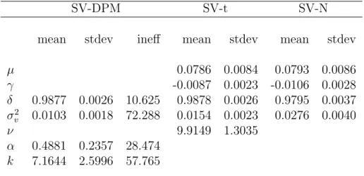
Table 1 reports the MCMC sample means and standard deviations for the parameters of the SV-DPM, SV-t, and SV-N models. We report the observed serial correlation in the draws of the SV-DPM models parameters with the ineﬃciency measure:

1 + 2 L ∑ τ=1 L−τ L ρ(τ),

where ρ(·) is the sample autocorrelation function of the parameter draws, L = 1000 is the largest lag at which the autocorrelation function is computed. The ineﬃciency measure quantiﬁes the loss associated with using correlated draws from the sampler, as opposed to truely independent draws, in computing the posterior mean. The numerical standard

(18)

error equals the square root of the product between the ineﬃciency measure and the sample variance of the draws (Geweke (1992)).

The posterior estimate of the variance of volatility parameter, σ_v2, is the smallest with the SV-DPM model. The posterior estimate of σ_v2 is 0.0103 with a standard deviation of 0.0018. This mean and standard deviation for σ2_v is substantially smaller than the SV-N models mean of 0.0276 and standard deviation of 0.004. For the SV-N model this is to be expected, given that the SV-N model requires a larger value of σ2

v in order to capture the

excess kurtosis found in the return data.

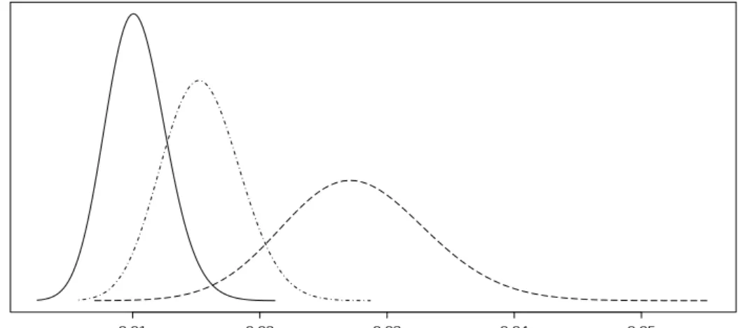
Excess kurtosis is still, however, unaccounted for by the SV-N return process (Bakshi et al. (1997), Chib et al. (2002)). A better characterization of the kurtosis is found in the SV-DPM and SV-t models where the distribution of the return process is ﬁt by a fat-tailed mixture of normals. Mixture models assign volatile time periods to draws from the tail of the return distribution rather than to a more volatile volatility process. As a resultσ_v2 in the SV-t model is smaller in value than in the SV-N model, but slightly larger than the SV-DPM, with a mean and standard deviation of 0.0154 and 0.0023. In Fig. 2 the posterior densities of σ_v2 are consistent with these observations. Notice the upper tail of the SV-DPM model’s density forσ_v2 barely overlaps with the lower tail of the SV-N model’s density, whereas there is considerable overlap with the lower tail of the SV-t model.

Dynamic behavior in volatility as captured by the AR-parameterδis nearly indistinguish-able between the three SV models. First-order dynamics in the volatility of the SV-DPM model is precisely estimated at 0.9887 with the tight posterior standard deviation of 0.0026. This estimate of δ is only slightly smaller than the SV-t estimate of 0.9878, but with the same posterior standard deviation. The volatility in the SV-N model reverts to its mean at a slightly faster pace with a posterior estimate of δ equal to 0.9795.

For the daily portfolio return the average SV-DPM mixture order isk = 7.16 and suggests that the SV-DPM not only captures the daily stock returns leptokurtotic behavior, but its skewness too. Because of the SV-N models symmetrical Gaussian innovations, it is unable to account for this asymmetrical behavior. Instead, it compensates for this skewness behavior by increasing its level of volatility during those periods where volatile is highest.

This increase in the volatility of the SV-N and SV-t model relative to the SV-DPM model is apparent in Figure 3 where the SV-DPM posterior conditional variance of returns is plotted in Panel (a) and the SV-DPM models diﬀerence from the conditional variances of the SV-N model are graphed in Panel (b) and the SV-t model in Panel (c). During those periods where the SV-DPM models conditional daily variance is greater than 2, the SV-N conditional variance is on the order of 2 to 14 points larger. The conditional variances of the SV-t model, while still greater than the SV-DPM model, only range from approximately 1 to 4 points larger than the SV-DPM variances.

(19)

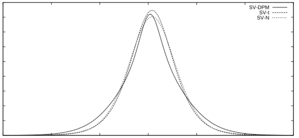
SV-N nor SV-t model is able to capture the skewness of daily returns. This is borne out in the one day ahead, out of sample, predictive density plots of Figure 4. The SV-DPM predictive density is clearly diﬀerent from the N or t models. For example, the SV-DPM predictive density is more centered around 0 and exhibits the asymmetry associated with the negative skewness of returns. In addition, the log-predictive densities plots of Figure 5 shows the SV-DPM producing fatter tails than either of the SV-N or SV-t model.

5.1 Robustness to DP hyperparameters

Using the same empirical data set of CRSP portfolio returns we estimate the SV-DPM model under five different prior specifications of π(α)≡ Γ(a, b) and G0 ≡N(m,(τ λ2t)−1)−

Γ(v0/2, s0/2) to test the robustness of the posterior estimates of the SV-DPM model to different priors. Table 2 reports these robustness findings for the posterior estimates of the SV-DPM model for the different priors.

To determine the impact the prior of the precision parameter has on the estimates of the SV-DPM model we evaluate the model under the prior speciﬁcation:

• Prior 2 : π(α)∼Γ(0.1,20),

whereE[α] = 0.005 and Var[α] = 0.00025, and leave the other priors exactly as before. These hyperparameter values cause the prior distribution for α to be more tightly distributed and centered closer to zero than did the original prior. As a result the posterior estimate of α

is found to be closer to zero at 0.1217. Since a smaller value for α lowers the probability of selecting a new cluster from the Polya urn, under Prior 2 the estimate of k is smaller at 4.4465. Though the mixture representation for the distribution of returns now on average consists of fewer clusters, notice that the posterior estimates of the volatility parameters, δ

and σ_v2, and their standard deviations are nearly the same as under the original prior. The only diﬀerence being the estimate ofσ2_v is slightly larger at 0.0112 with a standard deviation of 0.0019.

In the other four priors we allow the DP prior’s base distribution N(m,(τ λ2

t)−1) −

Γ(v0/2, s0/2) to change in order to explore how sensitive the posterior estimates of the SV-DPM model are to prior’s mean and spread. The four priors are:

• Prior 3 : G0 ≡N(0,(5∗λ2)−1)−Γ(10/2,10/2),

• Prior 4 : G0 ≡N(0,(15∗λ2)−1)−Γ(10/2,10/2),

• Prior 5 : G0 ≡N(0,(10∗λ2)−1)−Γ(5/2,5/2),

• Prior 6 : G0 ≡N(0,(10∗λ2)−1)−Γ(15/2,15/2),

where Prior 3 & 4 change the variance of the mixture mean, η, and Prior 5 & 6 tests for the robustness to changes in the prior of the mixture variance, λ2. In the posterior results reported in Table 2 neither of the changes in the hyperparameters to η nor λ2 base

(20)

distribution affect the posterior estimates of the SV-DPM model. Under each of the four priors the estimates of δ are the same up to the third decimal place at 0.978, and the estimates ofσ2_v are equal out to the second decimal place at 0.01. Subtle differences between the estimates of α can be found under the different priors, with the posterior estimates α

ranging from 0.4730 under Prior 4 to 0.4881 for the original prior. Similar results are found for k, where Prior 4 produces an estimate ofk = 6.9221, while k = 7.1644 for Prior 1.

5.2 Robustness to number of draws

Because the DPM sampler is a step-by-step algorithm, making 30,000 thinned draws from the SV-DPM model requires a considerable number of computing cycles. This is understandable given the level of ineﬃciency associated with the posterior draws of the SV-DPM model. It would, however, be preferable if a fewer number of draws could be used in making inference concerning the SV-DPM model. To determine if this is possible, the SV-DPM model for the CRSP portfolio return data is reestimated with a MCMC sample of 10,000 thinned draws. The posterior results of the SV-DPM model from these 10,000 draws are reported in Table 3. The table also includes the results from Table 1 where 30,000 draws were made. Notice that there is little diﬀerence between the posterior means of the parameters. The volatility parameters, δ and σ2

v, have comparable posterior means and exactly the same standard

deviations. The DP parametersα and k are also very similar.

5.3 Model comparison

The previous large sample analysis highlighted features of the predictive density that the standard parametric SV models could not account for. In this section we investigate the forecasting value of the predictive densites of the SV-DPM speciﬁcations in a small sample setting using 755 daily CRSP returns over the period January 3, 2006 to December 31, 2008. Given the existing results on the good performance of the basic parametric SV models we focus on the relative value that the new models contribute to density forecasts. To do this we use the model pooling approach of Geweke & Amisano (2008). This approach recognizes that none of the models may be the true DGP and advocates a linear prediction pool based on the log score function (predictive likelihood) from a set of models.

Given a set of predictive densities {f(yt|y1, . . . , yt−1, Mi)}Ki=1 from the set of models

{Mi}Ki=1 consider the combined predictive density of the form:

K ∑ i=1 wif(yt|y1, . . . , yt−1, Mi), K ∑ i=1 wi = 1, wi ≥0, i= 1, ..., K. (41)

Weights are chosen to maximize the log pooled, predictive score function: max wi,i=1,...,K τ2 ∑ t=τ1 log [ _K ∑ i=1 wif(yt|y1, . . . , yt−1, Mi) ] , (42)

(21)

where the predictive densities are evaluated at the realized data point yt.

For each of the models we run a MCMC simulation consisting of 11,000 draws of which the ﬁrst 1,000 draws are thrown away to obtain 10,000 posterior draws conditional on the return data up to time periodt−1; i.e.,y1, ..., yt−1. These draws are then used to estimate the predictive likelihoodf(yt|y1, . . . , yt−1, Mi).8 For the SV-DPM model the predictive likelihood

is estimated using Equation (35). MCMC draws of this size are carried out for each SV model and data sety1, . . . , yt−1 wheret =τ1, . . . , τ2. Given a history of predictive likelihood values for each model we can estimate the weights in Equation (42).

The pool of models considered are: SV-DPM; SV-DPM-λ; SV-t and SV-N; i.e., K = 4. Recall that in the SV-DPM-λ model of Section 2.1 only the return precision parameter λ2

t

is governed by the DP prior and the intercept is assumed to be the unknown constant µ. Conditional on return data back to January 3, 2006 (t = 1), we compute the log pooled predictive score function over the period of May 30, 2006 (τ1 = 105) to December 31, 2008 (τ2 = 755).9

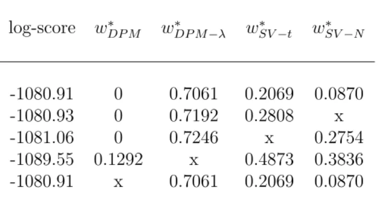
Table 4 displays the optimal log score and the weights for the linear pool of models. Using all four models the log score is −1080.91. The SV-DPM-λ model dominates with a weight of 0.71 followed by the SV-t model with 0.21. Each of the subsequent table entries drop one of the models from the pool to assess the deleted models relative importance towards forecasting as measured by the models contribution to the log score. As long as the SV-DPM-λ model is in the pool a similar log score is achieved but once this model is dropped the log score declines by over 8 points. The SV-DPM-λ nests both the SV-N and the SV-t model. The SV-t models a distinct precision parameter value for each observation, whereas the SV-DPM-λ models prior leads to a clustering of distinct precision parameter values that are fewer in number than the sample size.10 _{The zero or near zero weight and} lack of contribution to the pooled predictive likelihood function by the SV-DPM model is likely due to the fact that to learn about asymmetry in the return distribution requires more observations than our data series of 755 returns aﬀords.

6 Conclusion

This paper proposed a new Bayesian, semiparametric, autoregressive, stochastic volatility model where the conditional return distribution is modeled nonparametrically with an

in-8_{Because of the large number of predictive likelihoods that are required in the pooled predictive score}

function, the number of MCMC draws is smaller than the sampling performed in Section 5. For the largest series (745 observations) the SV-DPM sampler’s compiled C-code takes just over 6 minutes on a 3 GHz Intel Xeon quad-core computer running Linux.

9_{We decrease the computing time involved in calculating the pooled predictive score function by}

dis-tributing the calculation of each models 650 predictive likelihoods, f(yt|y1, . . . , yt−1), t = 105, . . . ,755, to

25-30 separate processors each using the same initial values.

(22)

ﬁnite ordered mixture of normal distributions. The unknown number of mixture clusters, their probability of occurrence, and their mean and variance are ﬂexibly modeled a prior

with a Dirichlet process prior. Conditional on a draw of the log-volatilities, an efficient MCMC algorithm has been constructed to produce posterior draws of the unknown number of mixture clusters and the clusters mean and variance. The sampler has been stress tested against existing parametric stochastic volatility models on real world daily return data. The semiparametric stochastic volatility model performed well on empirical return data, fitting both the negative skewness and leptokurtotic properties of returns, while still capturing the time-varying conditional heteroskedastic dynamics of returns. The semiparametric mod-els increased flexibility and robustness to non-Gaussian behavior and its superior forecasts makes it an appealing specification for risk and portfolio managers. The SV-DPM models can provide improvements in both large and small samples.

Important questions remain to be answered with the Bayesian semiparametric, stochastic volatility model. For instance, is it possible to attach structural meaning to the mixture parameters, such as a particular mixture cluster being identiﬁed with jumps in returns or to time periods where the economy is in a particular state of the business cycle? Placing such structural meaning on the mixture clusters is possible by assigning a prior rank ordering to the clusters within the Dirichlet process prior. Doing so overcomes the label switching problem discussed earlier.

Another area of potential research is that of leverage effects. Leverage effects have been used effectively with symmetrically distributed stochastic volatility models to produce neg-ative skewness in returns. A natural question one could ask is whether it is possible to introduce leverage effects into this paper’s semiparametric, stochastic volatility model. If so, how do leverage effects affect the skewness of the mixture distribution. These and other interesting questions remain for future research.

(23)

References

Bakshi, G., Cao, C. & Chen, Z. (1997), ‘Empirical performance of alternative options pricing models’, Journal of Finance 52(5), 2003–2049.

Blackwell, D. & MacQueen, J. (1973), ‘Ferguson distributions via polya urn schemes’, The Annals of Statistics 1, 353–355.

Chib, S. & Hamilton, B. (2002), ‘Semiparametric bayes analysis of longitudinal data treat-ment models’, Journal of Econometrics 110, 67–89.

Chib, S., Nardari, F. & Shephard, N. (2002), ‘Markov chain monte carlo methods for stochas-tic volatility models’,Journal of Econometrics 108(2), 281–316.

Clark, P. K. (1973), ‘A subordinated stochastic process model with ﬁnite variance for spec-ulative prices’, Econometrica 41(1), 135 – 155.

Conley, T., Hansen, C., McCulloch, R. & Rossi, P. (2008), ‘A semi-parametric bayesian approach to the instrumental variable problem’, Journal of Econometrics 144, 276– 305.

Durham, G. B. (2006), ‘Monte carlo methods for estimating, smoothing, and ﬁltering one-and two-factor stochastic volatility models’,Journal of Econometrics 133(1), 273–305. Elerian, O., Chib, S. & Shephard, N. (2001), ‘Likelihood inference for discretely observed

non-linear diﬀusions’,Econometrica 69(959–993).

Eraker, B., Johannes, M. S. & Polson, N. G. (2003), ‘The impact of jumps in volatility and returns’, Journal of Finance 58(3), 1269–1300.

Escobar, M. D. & West, M. (1995), ‘Bayesian density estimation and inference using mix-tures’, Journal of the American Statistical Association 90(430), 577–588.

Ferguson, T. (1973), ‘A bayesian analysis of some nonparametric problems’, The Annals of Statistics 1(2), 209–230.

Fleming, J. & Kirby, C. (2003), ‘A closer look at the relationship between garch and stochas-tic autoregressive volatility’, Journal of Financial Econometrics 1, 365–419.

Fr¨uhwirth-Schnatter, S. (2006),Finite Mixture and Markov Switching Models, Springer Series in Statistics. New York/Berlin/Heidelburg.

Gallant, A. R., Hsieh, D. & Tauchen, G. (1997), ‘Estimation of stochastic volatility models with diagnostics’, Journal of Econometrics 81, 159–192.

(24)

Gelfand, A. E. & Mukhopadhyay, S. (1995), ‘On nonparametric bayesian inference for the distribution of a random sample’, The Canadian Journal of Statistics 23(4), 411–420. Geweke (1994), ‘Comment on jacquier, polson and rossi’s ”bayesian analysis of stochastic

volatility models”’, Journal of Business & Economic Statistics 12, 389–392.

Geweke, J. (1992), Evaluating the accuracy of sampling based approaches to the calculation of posterior moments, in Bernardo, Berger, Dawid & Smith, eds, ‘Bayesian Statistics’, Vol. 4, Oxford: Clarendon Press.

Geweke, J. (2007), ‘Interpretation and inference in mixture models: Simple mcmc works’,

Computational Statistics & Data Analysis 51(7), 3529 – 3550.

Geweke, J. & Amisano, G. (2008), ‘Comparing and evaluating bayesian predictive distribu-tions of asset returns’, European Central Bank Working Paper 969.

Geweke, J. & Keane, M. (2007), ‘Smoothly mixing regressions’, Journal of Econometrics

138, 252–290.

Ghosal, S., Ghosh, J. & Ramamoorth, R. (1999), ‘Posterior consistency of dirichlet mixtures in density estimation’, Annals of Statistics 27(1), 143–158.

Ghosal, S. & van der Vaart, A. (2007), ‘Posterior convergence rates of dirichlet mixtures at smooth densities’, Annals of Statistics 35(2), 697–723.

Gonedes, R. C. B. N. J. (1974), ‘A comparison of the stable and student distributions as statistical models for stock prices’, The Journal of Business 47(2), 244–280.

Griﬃn, J. E. & Steel, M. (2006), ‘Order-based dependent dirichlet processes’, Journal of the American Statistical Association 101(473), 179–194.

Griﬃn, J. E. & Steel, M. F. J. (2004), ‘Semiparametric bayesian inference for stochastic frontier models’, Journal of Econometrics 123(1), 121–152.

Harvey, A., Ruiz, E. & Shephard, N. (1994), ‘Multivariate stochastic variance models’, The Review of Economic Studies 61(2), 247–264.

Hirano, K. (2002), ‘Semiparametric bayesian inference in autoregressive panel data models’,

Econometrica 70, 781–799.

Jacquier, E., Polson, N. G. & Rossi, P. E. (1994), ‘Bayesian analysis of stochastic volatility models’, Journal of Business & Economic Statistics 12, 371–417.

Jacquier, E., Polson, N. G. & Rossi, P. E. (2004), ‘Bayesian analysis of stochastic volatility models with fat-tails and correlated errors’, Journal of Econometrics 122, 185–212.