Syracuse University Syracuse University
SURFACE
SURFACE
Center for Policy Research Maxwell School of Citizenship and Public Affairs
1-2020
Forecasting with Unbalanced Panel Data
Forecasting with Unbalanced Panel Data
Badi Baltagi[email protected] Long Liu
University of Texas at San Antonio, [email protected]
Follow this and additional works at: https://surface.syr.edu/cpr
Part of the Economic Policy Commons, and the Economics Commons
Recommended Citation Recommended Citation
Baltagi, Badi and Liu, Long, "Forecasting with Unbalanced Panel Data" (2020). Center for Policy Research. 253.
https://surface.syr.edu/cpr/253
This Working Paper is brought to you for free and open access by the Maxwell School of Citizenship and Public Affairs at SURFACE. It has been accepted for inclusion in Center for Policy Research by an authorized administrator
Forecasting with Unbalanced
Panel Data
Badi Baltagi and Long Liu
Paper No. 221
CENTER FOR POLICY RESEARCH – Spring 2020
Leonard M. Lopoo, Director
Professor of Public Administration and International Affairs (PAIA) Associate Directors
Margaret Austin
Associate Director, Budget and Administration John Yinger
Trustee Professor of Economics (ECON) and Public Administration and International Affairs (PAIA) Associate Director, Center for Policy Research
SENIOR RESEARCH ASSOCIATES Badi Baltagi, ECON
Robert Bifulco, PAIA Leonard Burman, PAIA Carmen Carrión-Flores, ECON Alfonso Flores-Lagunes, ECON Sarah Hamersma, PAIA
Madonna Harrington Meyer, SOC Colleen Heflin, PAIA
William Horrace, ECON Yilin Hou, PAIA
Hugo Jales, ECON
Jeffrey Kubik, ECON Yoonseok Lee, ECON Amy Lutz, SOC Yingyi Ma, SOC
Katherine Michelmore, PAIA Jerry Miner, ECON
Shannon Monnat, SOC Jan Ondrich, ECON David Popp, PAIA Stuart Rosenthal, ECON Michah Rothbart, PAIA
Alexander Rothenberg, ECON Rebecca Schewe, SOC
Amy Ellen Schwartz, PAIA/ECON Ying Shi, PAIA
Saba Siddiki, PAIA Perry Singleton, ECON Yulong Wang, ECON Michael Wasylenko, ECON Peter Wilcoxen, PAIA Maria Zhu, ECON GRADUATE ASSOCIATES
Rhea Acuña, PAIA
Mariah Brennan, SOC. SCI. Jun Cai, ECON
Ziqiao Chen, PAIA Yoon Jung Choi, PAIA Dahae Choo, PAIA Stephanie Coffey, ECON Brandon De Bruhl, PAIA Giuseppe Germinario, ECON Myriam Gregoire-Zawilski, PAIA Emily Gutierrez, PAIA
Jeehee Han, PAIA Mary Helander, Lerner Hyoung Kwon, PAIA Mattie Mackenzie-Liu, PAIA Maeve Maloney, ECON
Austin McNeill Brown, SOC. SCI. Qasim Mehdi, PAIA
Claire Pendergrast, SOC Jonathan Presler, ECON Krushna Ranaware, SOC
Christopher Rick, PAIA David Schwegman, PAIA Saied Toossi, PAIA Huong Tran, ECON Joaquin Urrego, ECON Yao Wang, ECON Yi Yang, ECON Xiaoyan Zhang, ECON Bo Zheng, PAIA
Dongmei Zhu, SOC. SCI.
STAFF Joanna Bailey, Research Associate
Joseph Boskovski, Manager, Maxwell X Lab Katrina Fiacchi, Administrative Specialist
Emily Minnoe, Administrative Assistant Candi Patterson, Computer Consultant Samantha Trajkovski, Postdoctoral Scholar
Abstract
This paper derives the best linear unbiased prediction (BLUP) for an unbalanced panel data model. Starting with a simple error component regression model with unbalanced panel data and random effects, it generalizes the BLUP derived by Taub (1979) to unbalanced panels. Next it derives the BLUP for an unequally spaced panel data model with serial correlation of the AR(1) type in the remainder disturbances considered by Baltagi and Wu (1999). This in turn extends the BLUP for a panel data model with AR(1) type remainder disturbances derived by Baltagi and Li (1992) from the balanced to the unequally spaced panel data case. The derivations are easily implemented and reduce to tractable expressions using an extension of the Fuller and Battese (1974) transformation from the balanced to the unbalanced panel data case.
.JEL No.: C33
Keywords: Forecasting, BLUP, Unbalanced Panel Data, Unequally Spaced Panels, Serial Correlation
Authors: Badi H. Baltagi, Department of Economics, Center for Policy Research, 426 Eggers Hall, Syracuse University, Syracuse, NY 13244-1020, [email protected]; Long Liu, Department of Economics, College of Business, University of Texas at San Antonio, 1 UTSA Circle, TX 78249-0633, [email protected]
1
Introduction
Panel data is usually unbalanced or unequally spaced due to lack observations on house-holds not interviewed in certain years or firms not filing their data survey forms for a particular period. Even daily stock price data has no observations when the market is closed due to holidays or weekends. The unequally spaced pattern is also useful for re-peated sales of houses that are not sold each year but at irregularly spaced intervals. It is also a common problem for longitudinal surveys and household surveys in developed as well as developing countries, see examples of these in Table 1 of McKenzie (2001) as well as Table 1 of Millimet and McDonough (2017). Unbalanced panel data estimation and testing has been studied in econometrics, see Chapter 9 of Baltagi (2013a) and the references cited there. This paper focuses on forecasting with unbalanced panel data. In particular, the paper starts by extending the best linear unbiased predictor (BLUP) derived by Taub (1979) for the random effects error component model from balanced to unbalanced panel data models. Next, the BLUP for the unequally spaced panel data with serial correlation of the AR(1) type in the remainder disturbances, considered by Baltagi and Wu (1999) is derived. This extends the BLUP for the random effects model with serial correlation of the AR(1) type derived by Baltagi and Li (1992) from balanced panels to unequally spaced panels. Unbalanced panel data can be messy. This paper keeps the derivations simple and easily tractable, using the Fuller and Battese (1974) transformation extended from the balanced to the unbalanced panel data case.
2
The Best Linear Unbiased Predictor
Consider an unbalanced panel data regression model:
yit=Xit0β+uit (1)
for i = 1, . . . , N; t = 1. . . , Ti. The i subscript denotes, say, individuals in the
cross-section dimension and t denotes years in the time-series dimension. The panel data is unbalanced since there areN unique individuals and individualiis only observed overTi
time periods.1 The regressor X
it is a K×1 vector of the explanatory variables and β is
a K ×1 vector of coefficients. In an earnings equation in economics, for example, yit is
log wage for theith worker in the tth time period. Xit may contain a set of variables like
age, experience, tenure, and whether the worker is male, black, etc. In most of the panel data applications, the disturbances follow a simple one-way error component model with
uit=µi+vit (2)
whereµi denotes theunobservable time-invariant individual specific effect, such as ability.
vit denotes the remainder disturbance that varies with individuals and time, see Baltagi
P
(2013a) . Let n= Ni=1Ti. In vector notation, Equations (1) and (2) can be written as
y =Xβ+u (3)
and
u=Zµµ+v (4)
where y = (y11,. . . , y1T1, y , . . . , y21 2T2, . . . , yN1, . . . , yN TN) is an0 n× 1 vector of ,obser-vations stacked such that the slower index is over individuals and the faster index is over time.2 Other vectors or matrices including X, u and v are similarly defined. µ = (µ1, . . . , µN)0 is anN×1 vector. The selector matrixZµ =diag[ιTi] is a matrix of ones and zeros, where ιTi is a vector of ones of dimension Ti. It is simply the matrix of individual dummies that one may include in the regression to estimate the µi if they are assumed
1The data is assumed to be missing at random. This in turn allows the missingness of the data scheme
to be ignorable in the language of Little and Rubin (2002).
2This pattern of unbalancedness does not have to be from 1,2, .., T
i. In fact, theseTiobservations can
be for any subset of the observed time series period. This pattern is used to make the derivation easy and tractable and follow similar derivations for the balanced case. A more general pattern of unbalancedness can be used. In fact, section 2 extends this to the unequally spaced panel data with serial correlation across time considered by Baltagi and Wu (1999). A two-way error component model with a general type of missing data is considered in Wansbeek and Kapteyn (1989).
to be fixed parameters. Define P = Zµ(Zµ0Zµ)−1Zµ0, which is the projection matrix on
Zµ. In this case, ZµZµ0 = diag[JTi], where JT is a matrix of ones of dimension Ti. Let
i
¯ ¯
JTi =JTi/Ti. Hence P reduces to diag JTi , which averages the observation across time for each individual over their Ti observations. Similarly, Q=IN T −P is a matrix which
obtains the deviations from individual means. For example, if we regress yon the matrix
P
of dummy variables Zµ, the predicted values P y have a typical elementyi. = Ti
t=1yit/Ti
repeatedTitimes for each individual. Qygives the residuals of this regression with typical
element yit−yi..
For therandom effects model,µi ∼IID(0, σ2µ),vit ∼IID(0, σν2) and theµi are
indepen-dent of thevit and Xit for all iand t. The variance-covariance matrix of the disturbances
is given by Ω =E(uu0) = σ2µdiag[JTi] +σ 2 vdiag[ITi] =diag ωi2J¯Ti +σ 2 νETi (5) ¯ ¯
whereωi2 =Tiσµ2+σν2,andETi =ITi−JTi. Using the fact thatJTi andETi are idempotent matrices that sum to the identity matrix I ,Ti it is easy to verify that
Ω−1 =diag 1 ω2 i ¯ JTi + 1 σ2 ν ETi (6) and Ω−1/2 =diag 1 ωi ¯ JTi+ 1 σν ETi (7) see Wansbeek and Kapteyn (1982). Now a GLS estimator can be obtained as a weighted least squares following Fuller and Battese (1974). In this case one premultiplies the
h i
¯ ¯
regression model in Equation (3) by σνΩ−1/2 = diag σωνiJTi +ETi = diag ITi−θiJTi where θi = 1−(σν/ωi). GLS becomes OLS on the resulting transformed regression of y∗
on X∗ with y∗ =σνΩ−1/2y having a typical element yit∗ =y
∗ −1/2
it−θiy¯i.,and X =σνΩ X
defined similarly.
(1962), the best linear unbiased predictor (BLUP) of yi,Ti+S for the GLS model is ˆ yi,Ti+S =X 0 i,Ti+SβGLS +w 0 Ω−1uˆGLS, ˆ (8) ˆ
forS >1, whereβGLS is the GLS estimator ofβ from equation (3),w=E(ui,T+Su), Ω is
the variance-covariance structure of the disturbances, andubGLS =y−XβˆGLS. Note that
we haveui,Ti+S =µi+ν
0 2 0
i,Ti+S for period Ti+S and hencew =σµ(0, .., ιTi,0, ..,0). In this case w0Ω−1 =σ2µ(0, .., ι0T i,0, ..,0)diag 1 ω2 i ¯ JTi + 1 σ2 ν ETi = σ2µ ω2 i (0, .., ι0T i,0, ..,0) (9) since ι0T i ¯ JTi =ι 0 Ti and ι 0
TiETi = 0. The last term of BLUP becomes
w0Ω−1buGLS = Tiσ2µ ω2 i b ui.,GLS, (10) P
where bui.,GLS = Ti−1 tT=1i ubit,GLS. Therefore, the BLUP for yi,T+S corrects the GLS
prediction by a fraction of the mean of the GLS residuals corresponding to that ith individual over the Ti observed periods. This BLUP was derived by Taub (1979) for the
balanced panel data case. Note that it is based on the true variance components. In practice, we need to estimate the variance components to get feasible GLS and a feasible BLUP. Methods for estimating the variance components for the unbalanced panel data model are described in more details in Baltagi (2013a). To account for the additional uncertainty introduced by estimating these variance components, Kackar and Harville (1984) proposed inflation factors for the predictor.
Although this derivation has albeit a restrictive form of missing observations, for example, the time series has no gaps, the results still hold for the Fuller and Battese (1974) transformation and the Goldberger (1962) BLUP derivation even with time series gaps. This is because the individual effects are independent and the idiosyncratic error terms are not correlated across time. Also, as footnote 2 states, the pattern of missing observations can be more general, all that matters is that individual i be observed for only Ti periods and these can be any subset of the observed sample period.
For a recent survey of the BLUP literature mostly for balanced panel data in economet-rics, see Baltagi (2013b). The BLUP methodology in statistics has been used extensively
in biometrics, see Henderson (1975). Harville (1976) showed that BLUP is equivalent to Bayesian posterior mean predictors with a diffuse prior. Robinson (1991) has an extensive review of how BLUP can be used for example to remove noise from images and for small-area estimation. It can be also used to derive the Kalman filter. For several applications of forecasting with panel data in economics and related disciplines, see the handbook of forecasting chapter by Baltagi (2013b) and the references cited there.
In the next section, we revisit the unequally spaced panel data model with AR(1) type remainder disturbances, considered by Baltagi and Wu (1999). While the Fuller and Battese (1974) transformation for that model was derived in that paper, the Goldberger (1962) BLUP was not given. For forecasting purposes, we derive a simple to compute expression of this predictor and show that it reduces to the usual BLUP under several special cases.
3
Unequally Spaced Panel Data Model with AR(1)
type remainder disturbances
Baltagi and Wu (1999) considered an unequally spaced panel data model withbothrandom effects and serial correlation of the AR(1) type in the remainder disturbances. To be specific, µi ∼ IID(0, σµ2) and is assumed to be independent of the remainder disturbances
vit. In this case, vit follows an AR(1) process given by
vit =ρvi,t−1+it (11)
for t = 1, .., Ti, where it ∼ IID(0, σ2) and |ρ| <1. For the initial value, we assume vi0 ∼
(0, σ2
/(1−ρ2)). For each individuali, one observes the data at timesti,j forj = 1, . . . , ni.
Furthermore, we have 1 = ti,1 < · · · < ti,ni = Ti for i = 1, . . . , N with ni > K. This is a general form of unbalanced panel data which encompasses the case in Section 1. For
i= 1, . . . , N, we have
whereu0i = ui,ti,1, . . . , u
0
i,ti,ni , vi = vi,ti,1, . . . , vi,ti,ni and ιni is a vector of ones of dimen-sion ni. In vector forms, the disturbance term in Equation (12) can be written as
u=diag[ιni]µ+ν, (13) where u= (u1, . . . , uN), µ= (µ1, . . . , µN) and v0 = (v10, . . . , v
0
N). The variance-covariance
matrix of u is Ω = E(uu0) =diag[Λi], where Λi =E(uiu0i) =σµ2Jni +Vi, Jni is a matrix of ones of dimension ni, and Vi =E(vivi0). For any two observed periods, say ti,j and ti,l,
| |
the covariance term is given bycov v , vi,ti,l =σ
2 ti,j−ti,l
i,ti,j ρ /(1−ρ2) forj, l = 1, . . . , ni.
To remove the serial correlation in vit and keep it homoskedastic, Baltagi and Wu (1999)
introduced an ni×ni transformation matrix Ci∗(ρ), which is given by
Ci∗(ρ) = 1−ρ2 1/2 (14) × 1 0 · · · 0 0 −ρti,2−ti,1 1−ρ2(ti,2−ti,1)1/2 1 1−ρ2(ti,2−ti,1)1/2 · · · 0 0 .. . ... . .. ... ... 0 0 · · · −ρti,ni−ti,ni−1 1−ρ2(ti,ni−ti,ni−1) 1/2 1 1−ρ2(ti,ni−ti,ni−1) 1/2 .
Premultiplying Equation (12) byCi∗(ρ), we get the transformed error
u∗i =Ci∗(ρ)ui =µigi+Ci∗(ρ)νi, (15) where gi =Ci∗(ρ)ιni = 1−ρ 21/2 1, 1−ρti,2−ti,1 1−ρ2(ti,2−ti,1)1/2 ,· · · , 1−ρ ti,ni−ti,ni−1 1−ρ2(ti,ni−ti,ni−1)1/2 . (16) Baltagi and Wu (1999) showed that C∗(ρ)ν ∼ (0, σ2I ), i.e., C∗(ρ)V C∗ 0
i i ni i i i (ρ) = σ2Ini. The variance-covariance matrix for the transformed disturbance u∗ = (u∗1, . . . , u∗N) is Ω∗ =diag[Λ∗i], where Λ∗i =Ci∗(ρ) ΛiCi∗(ρ) 0 =σµ2gigi0+σ2Ini =ω 2 iPgi +σ 2 Qgi, (17) with ω2 i = g 0 igiσµ2 +σ2, P 0 −1 0
gi = gi(gigi) gi, Qgi = Ini −Pgi and Ini is an identity matrix of dimension ni. Using the fact that Pgi and Qgi are idempotent matrices which are
orthogonal to each other, we have Λ∗−1i /2 = ωi2 −1/2Pgi+ σ 2 −1/2 Qgi = σ 2 −1/2 Ini− σ 2 −1/2 − ω2i −1/2 Pgi. h i (18) h ∗− Hence, σ /2 1 Ω∗−1 1/2 ∗− /2
= diag σΛi , where σΛi = Ini − θiPgi and θi = 1 −σ/ωi. Premultiplying y∗ = diag[Ci∗(ρ)]y by σΩ∗−1/2, one gets y∗∗=σΩ∗−1/2y∗. The elements
of y∗∗ are given by
i
yi,t∗∗i,j =yi,t∗i,j −θigi,j ni s=1gi,sy ∗ i,ti,s Pni s=1gi,s2 . P (19) Baltagi and Wu (1999) proposed estimating σ2
µ and σ2 by ˆ σ2µ= u ∗0diag[P gi]u ∗−Nσˆ2 PN i=1g 0 igi and ˆσ2 = u ∗0diag[Q gi]u ∗ PN i=1(ni−1) . (20)
Since the true disturbances u∗ are unknown, we use u˜∗OLS instead, which are the OLS residuals from the (*) transformed equation. In order to make the (*) transformation operational, we need an estimate of ρ. Let v˜ be the within residuals from y on X. Inserting zeros between v˜i,ti,j and v˜i,ti,j+1 if the data between these two periods are not
available, one gets a new T ×1 residual ei. An estimate of ρ can be obtained as
ˆ ρ= 1 m N i=1 T t=2eitei,t−1 1 n i=1 t=1 it P
where m = Ni=1mi, mi is the number of observed consecutive pairs for each individual
P i and n= Ni=1ni. PN PT e2 , P P (21)
Theorem 1 Assume that (i) it ∼ iid(0, σ2); (ii) i=1v
2 i0 = O(1); (iii) N N i=1µ 2 i = We have ρˆ−ρ=op(1). 1 PN 1 PN O(1); (iv) Nm →0.
The proof is given in the Appendix. Assumptions (i), (ii) and (iii) were used in Hahn
P
and Kuersteiner (2002). Assumption (iv) Nm →0 is equivalent to mN = N1 Ni=1mi → ∞.
The consistency of ρˆ requires the average number of observed consecutive pairs to be large. For balanced panel data, this condition reduces to T → ∞. Using this estimator
of ρ, one gets a feasible GLS estimator of β. Detailed steps can be found in Baltagi and Wu (1999).3
Now, we return to prediction. Using the fact that the disturbances are independent across different individuals, we havew0 =E(ui,T+Su0) = (0, .., E(ui,Ti+Su0i),0, ..,0), which is a vector of zeros except for the ith position. Therefore,
0 − 0 wΩ 1 = (0, .., E(ui,Ti+Sui),0, ..,0)diag Λ −1 i = 0, .., E(u 0 −1 i,Ti+Sui) Λi ,0, ..,0 (22) and w0Ω−1uˆGLS = 0, .., E(ui,Ti+Su 0 i) Λ −1 i ,0, ..,0 ˆ u1 ˆ u2 .. . ˆ uN =E(ui,Ti+Su 0 i) Λ −1 i uˆi, (23)
whereu0i = ui,ti,1, . . . , ui,ti,ni andubidenote the GLS residuals. Sinceui,Ti+S =µi+νi,Ti+S, we can decompose equation (23) into two terms:
E(ui,Ti+Su 0 i) Λ −1 i uˆi =E(µiu0i) Λ −1 i uˆi+E(vi,Ti+Su 0 i) Λ −1 i uˆi. (24) Since Λ∗i =Ci∗(ρ) ΛiCi∗(ρ) 0 , we have Λ−1i =Ci∗(ρ)0Λ∗−1i Ci∗(ρ) =Ci∗(ρ)0 ωi−2Pgi +σ −2 Qgi Ci∗(ρ) (25) using Equation (18). Since µi and vi are independent of each other, we have E(µiu0i) =
E µiµiι0ni =σ
2
µι
0
ni. The first term in equation (24) can be rewritten as:
E(µiu0i) Λ −1 i uˆi = σµ2ι0n iC ∗ i (ρ) 0 ω−2i Pgi+σ −2 Qgi Ci∗(ρ) ˆui = σ 2 µ ω2g 0 iuˆ ∗ i, i (26)
3It is important to note that this is easily programmable. In fact, the Baltagi and Wu (1999) feasible
GLS procedure has been implemented in Stata using xtregar, so it is easy to derive the BLUP from these results.
where Ci∗(ρ)uˆi =uˆ∗i, using the fact C ∗ i (ρ)ιni =gi, g 0 iPgi =g 0 i and g 0 iQgi = 0.By continu-ous substitution, we have
vi,Ti+S =ρ Sv i,Ti+ρ S−1 i,Ti+1+· · ·+i,Ti+S and
E(vi,Ti+Su0i) = E(vi,Ti+S iv0) =E ρSvi,Ti+ρS−1i,Ti+1+· · ·+
0 i,Ti+S vi =ρ SE(v i,Tiv 0 i) since E[i,Ti+1v 0 i] = · · · = E[i,Ti+Sv 0 i] = 0. Because E(vi,Tiv 0
i) is the last column of the
covariance matrix E(viv0i) =Vi, we have
E(vi,T+Su0i) = ρ
S(0,· · · ,0,1)V i.
Also,Λ−1i in Equation (25) reduces to Λ−1i = Ci∗(ρ)0 ωi−2Pgi +σ −2 Qgi Ci∗(ρ) = Ci∗(ρ)0 σ−2Ini− σ −2 −ω −2 i Pgi Ci∗(ρ) = Ci∗(ρ)0 σ−2Ini− g0 igiσµ2 σ2 ωi2 gi(gi0gi) −1 g0i Ci∗(ρ) = σ−2Ci∗(ρ)0Ci∗(ρ) Ini − σµ2 ω2 i ιnig 0 iC ∗ i (ρ)
using the fact thatQgi =Ini−Pgi,ω
2
i =g
0
igiσµ2+σ2 and gi =Ci∗(ρ)ιni. The second term in equation (24) becomes: E(vi,Ti+Su 0 i) Λ −1 i uˆi = ρS(0,· · · ,0,1)Viσ−2 C ∗ i (ρ) 0 Ci∗(ρ) Ini− σ2 µ ω2 i ιnig 0 iC ∗ i (ρ) ˆ ui = ρS(0,· · · ,0,1) ˆ ui − σ2 µ ω2 i ιnig 0 iuˆ ∗ i = ρSuˆi,Ti − ρSσ2 µ ω2 g 0 iuˆ ∗ i i (27) −1
using the fact that σ−2V = C∗(ρ)0C∗ ∗ ∗ 0 2
equations (26) and (27), one gets w0Ω−1uˆGLS = ρSuˆi,Ti + 1−ρS σ2 µ ω2 i gi0uˆ∗i = ρSuˆi,Ti + 1−ρS (1−ρ2)1/2σ2 µ ω2 i " ˆ u∗i,ti,1 + ni X j=2 1−ρti,j−ti,j−1 1−ρ2(ti,j−ti,j−1)1/2 ˆ u∗i,ti,j # . (28) Special case 1: No missing observations. This is the balanced panel data model with AR(1) remainder disturbance terms considered by Baltagi and Li (1992). In this case, we haveti,j−ti,j−1 = 1, Ti =ni =T,
gi = 1−ρ2 1/2 1, 1−ρ (1−ρ2)1/2,· · · , 1−ρ (1−ρ2)1/2 = (1−ρ)ι α T, ! p where ια T = (α,1,· · · ,1) withα = (1 +ρ)/(1−ρ). gi0gi = (1−ρ) 2 d2,
and d2 =α2+T −1. Henceωi2 =σ2α, where σα2 = (1−ρ)2d2σµ2 +σ2. 1−ρti,j−ti,j−1 1−ρ
1/2 = ,
1−ρ2(ti,j−ti,j−1) (1−ρ2)1/2
ub∗i =Cubi, whereC is the T ×T Prais-Winsten (PW) transformation matrix
C = (1−ρ2)1/2 0 0 · · · 0 0 −ρ 1 0 · · · 0 0 .. . ... ... . .. ... ... 0 0 0 · · · 1 0 0 0 0 · · · −ρ 1 .
Therefore, Equation (28) reduces to
w0Ω−1ubGLS =ρSbui,T + (1−ρ) 1−ρS σ2 µ σ2 αub ∗ i1+ T t=2ub ∗ it . α
This is Goldberger’s BLUP extra term derived by Baltagi and Li (1992). So, the unbal-anced panel Goldberger’s BLUP correction term reduces to its balunbal-anced panel counterpart in the case of AR(1) remainder disturbance terms.
Special case 2: No random effects. This reduces to a panel data model without individual effects, but with AR(1) remainder disturbances. In this case σµ2 = 0, and equation (28) reduces to
w0Ω−1uˆGLS =ρSuˆi,Ti. (29) This is Goldberger’s BLUP extra term for the unbalanced panel data model with AR(1) remainder disturbances but no random individual effects. Goldberger (1962) actually con-sidered a simple time series regression (not a panel) with AR(1) remainder disturbances. Special case 3: No serial correlation. This is the unbalanced random effects model without serial correlation in Section 1. In this caseρ= 0,gi =ιni,g
0
igi =ni,ωi2 =niσµ2+σ2
and uˆ∗it =uˆit. Equation (28) in this case reduces to
w0Ω−1uˆGLS = σ2 µ ω2 i ni X j=1 ˆ ui,ti,j = niσµ2 ω2 i b ui.,GLS, (30) where ubi.,GLS =n−1 ni
i j=1uˆi,ti,j. This is Goldberger’s BLUP extra term for the unequally spaced panel data model with no serial correlation. This encompasses the case derived in Section 1 with ni = Ti, ωi2 = Tiσµ2 +σ2 and the extra BLUP Goldberger (1962) term
reduces to the one given in Equation (10).
P
4
Monte Carlo Simulation
To study the finite sample performance of the proposed estimator of ρ as well as the performance of the corresponding predictors, we perform Monte Carlo experiments in this section. Following Baltagi, Chang and Li (1992) but with random effects, we generate the following panel model
yit= 1 +xit+µi+vit, (31)
for i= 1, . . . , N; t= 1. . . , T + 1, where xit= 0.1t+ 0.5xi,t−1+wit. wit follows a uniform
distribution [−0.5,0.5] and xi0 = 5 + 10wi0. The individual specific effects are generated
iid
as µi ∼ N(0,10) and the remainder error follows an AR(1) process vit = ρvi,t−1 +it, iid
et al. (1992), one can translate this starting date into an “effective” initial variance assumption regardless of when the AR(l) process started. More specifically, to check
iid
the impact the of the initial condition, we let vi0 ∼ N(0, τ /(1−ρ2)) where τ varies over the set {0.2,1,5}. We generate the estimation sample such that the average time
¯
period observed is T = 1 PN
i=1Ti = 5, 10, 20 or 40. As shown in Table 1, we consider
N
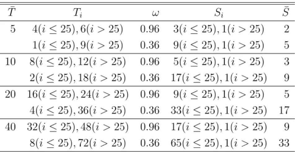
four different unbalanced panel data designs that are similar to those in Bruno (2005). In each design, the Ahrens and Pincus (1981) index ω, which measures the extent of unbalancedness, is set to be 0.36 or 0.96.4 In all experiments, the number of individuals is always N = 50. We perform 1,000 replications for each experiment.
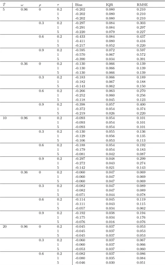
Table 2 reports the bias, interquantile range (IQR), and root mean squared error (RMSE) of the estimator of ρ. Following Kelejian and Prucha (1999), bias is calculated as the difference between the median and the true parameter value;IQR is the difference
1/2
between the 0.75 and 0.25 quantiles; and RM SE = bias2+ (IQR/1.35)2
. These measures are always assured to exist, see Kelejian and Prucha (1999) for details. As
¯ ¯
shown in Table 2, when T is small, ρˆ has negative bias. However, the bias shrinks as T
increases. Whenρ >0, the bias, IQR and RMSE all decrease when τ increases.
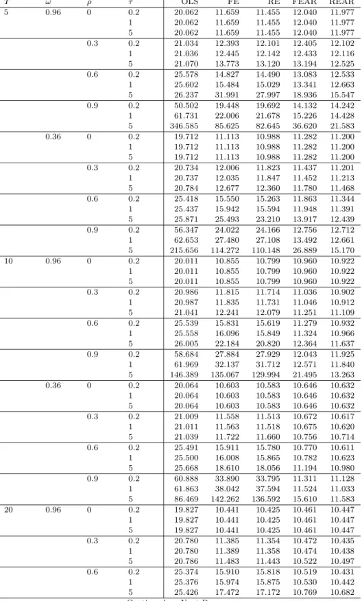
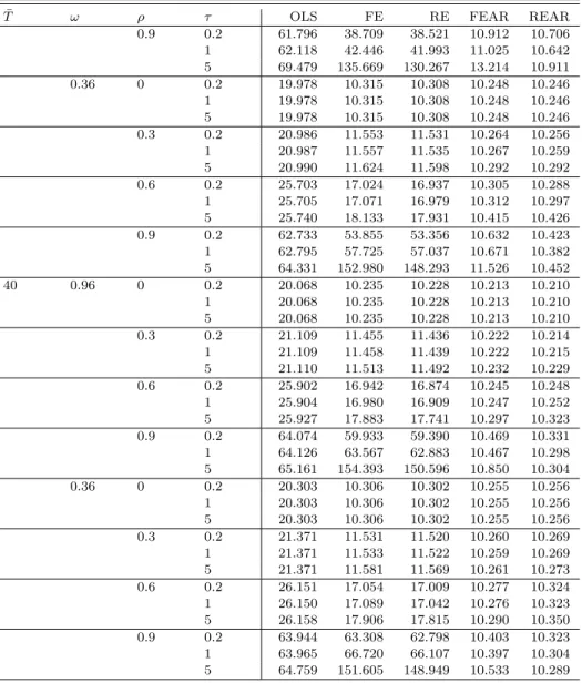
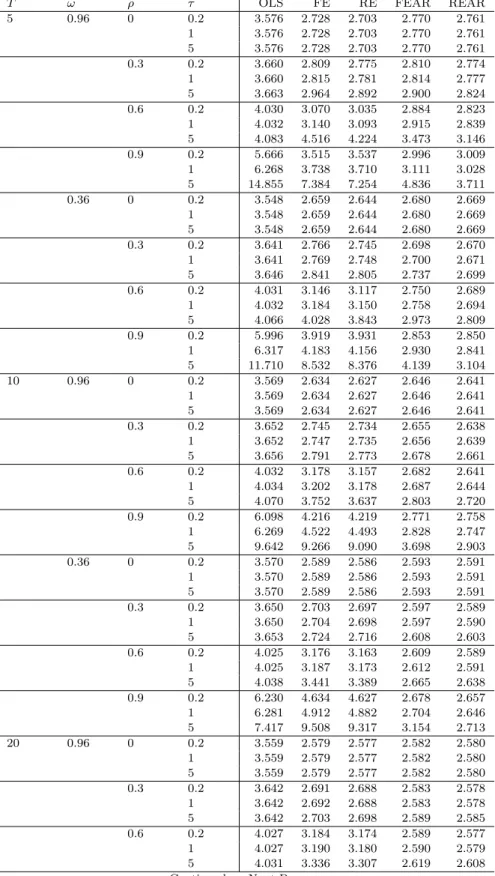
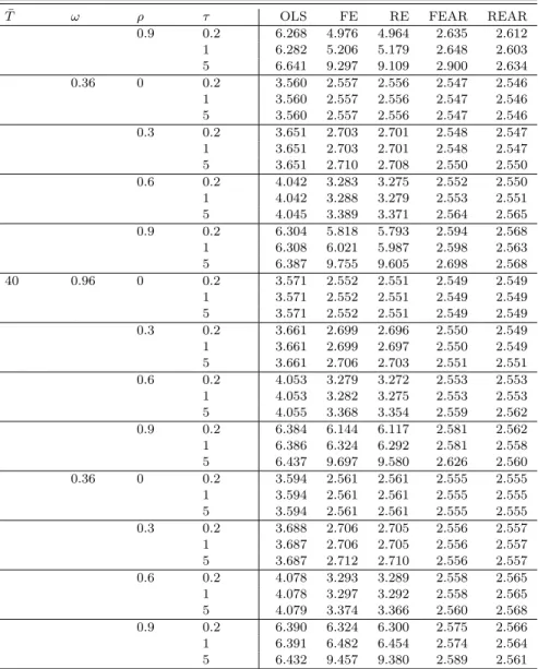
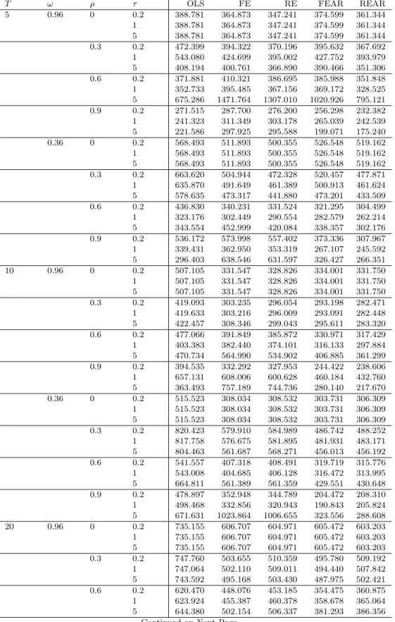
Tables 3-5 report the prediction performance of the following estimators: the pooled ordinary least squares (OLS), panel fixed-effects (FE) and random effects (RE) estimators that ignore autocorrelations in the error terms, and the fixed-effects and random effects estimators with AR(1) term, which are denoted as FEAR and REAR respectively. To summarize the accuracy of the forecasts, following Baltagi and Liu (2013a), we report the sampling mean square error (MSE), the mean absolute error (MAE) and the mean absolute percentage error (MAPE), which are computed as
M SE= 1 N R R X r=1 N X i=1 d2i,Ti+Si, (32)
4See also Baltagi and Chang (1995) for more discussion on incomplete panels and this Ahrens and
P
¯ N
Pincus measure. Note that ω = N/(T i=1Ti−1), with 0< ω ≤ 1. When the panel data is balanced
M AE = 1 N R R X r=1 N X i=1 |di,Ti+Si| (33) and M AP E = 100 N R R X r=1 N X i=1 di,Ti+Si yi,Ti+Si , (34)
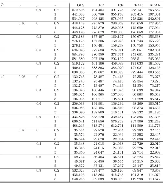
where di,Ti+Si = yˆi,Ti+Si −yi,Ti+Si, R = 1,000 replications and we forecast the last year available for individual i.5 As shown in Tables 3-5, REAR usually has the smallest MSE and MAE when ρ > 0. However, FEAR sometimes has a smaller MAPE than REAR even though the true DGP is created to be a random effect model with an AR(1) error term.
5
Application
In this section we illustrate the BLUP forecasts using an extract from the National Lon-gitudinal Study data set employed by Drukker (2003). This is an unbalanced panel data over the years 1968-1988 with gaps. The data is used to illustrate the xtreg command in Stata and includes observations on wages for 4711 young working women who were 14–26 years of age in 1968, some with only one observation. We regressed the loga-rithm of wage (lnwage) on the woman’s age and its square (age, age2), total working experience (exp), tenure at current position and its square (tenure, tenure2), current grade completed (grade), a dummy variable for not living in a standard metropolitan statistical area (nsmsa), a dummy variable for living in the south (south) and a dummy variable for black (black).6 we estimate the model by using the pooled OLS, FE, RE,
5It is worth pointing out that forecasting is not always one period ahead, as it varies by individual
depending on the missing observations. In fact, the last available year for a particular individual could sometimes be several years ahead due to irregular gaps of missing data between years. This is why we gave the expression for the BLUP forecast forSi periods ahead for individuali.
6Drukker (2003) uses this data to estimate an earnings equation to illustrate a test for serial correlation
proposed by Wooldridge (2002). Experience squared was not significant and was dropped from the regression. Zero serial correlation of the first order was rejected.
FEAR and REAR respectively. In order to compute the forecasts, we focus on women who had records for at least three years. For each estimator, we compute the forecast of the logarithm of wage for the last available year for that individual. This year is not used in the estimation but is used in the computation of the three forecast performance measures. To summarize the accuracy of the forecasts, we report MSE, MAE and MAPE, which are defined in Equation (32)-(34) with R = 1. As shown in Table 6, the random effects model with an AR(1) term has the smallest MSE or MAE. While, the fixed-effects model with an AR(1) term has the smallest MAPE. This is consistent with the findings in the simulation results. For time series data sets, Diebold and Mariano (1995) derived a test to compare prediction accuracy. Recently, Timmermann and Zhu (2019) extend the Diebold and Mariano (1995) test to panel data to compare the significance of pairwise forecasts averaged over all cross-sectional units. The results of this panel data test of equal predictive accuracy is reported in Table 7. Overall, the random effects model with an AR(1) term predicts significantly better than all other models.
6
Conclusion
This paper derives the BLUP for the unbalanced panel data model and the unequally spaced panel data model with AR(1) remainder disturbances and illustrates these with an earnings equation using the NLS young women data over the period 1968-1988 em-ployed by Drukker (2003) using Stata. These results can be extended to the unbalanced panel data model with AR(p) remainder disturbances, see Baltagi and Liu (2013a) for the corresponding balanced panel data case. Also, the unbalanced panel data model with MA(q) remainder disturbances, see Baltagi and Liu (2013b) for the corresponding balanced panel data case. Another extension is for the autoregressive moving average ARMA(p, q) remainder disturbances, see Galbraith and Zinde-Walsh (1995) for the bal-anced panel data case.
Data Availability Statement
The data used in the paper are available on the Stata web site for all Stata users.
References
Ahrens, H. and R. Pincus, 1981, On two measures of unbalancedness in a one-way model and their
relation to efficiency, Biometric Journal, 23, 227-235.
Baltagi, B.H., 2013a. Econometric analysis of panel data, Wiley and Sons, Chichester.
Baltagi, B.H., 2013b, Panel data forecasting, chapter 18 in the handbook of economic forecasting,
Volume 2B, edited by Graham Elliott and Allan Timmermann, North Holland, Amsterdam,
995-1024.
Baltagi, B.H. and Y.J., Chang, 1995, Incomplete panels, Journal of Econometrics, 62, 67–89.
Baltagi, B.H., Chang, Y.J., and Q. Li, 1992, Monte Carlo evidence on panel data regressions with AR
(1) disturbances and an arbitrary variance on the initial observations, Journal of Econometrics,
52(3), 371-380.
Baltagi, B.H. and Q. Li, 1992, Prediction in the one-way error component model with serial correlation,
Journal of Forecasting 11, 561–567.
Baltagi, B.H. and L. Liu, 2013a, Estimation and prediction in the random effects model with AR(p)
remainder disturbances, International Journal of Forecasting 29, 100-107.
Baltagi, B.H. and L. Liu, 2013b, Prediction in the random effects model with MA(q) remainder
distur-bances, Journal of Forecasting 32, 333-338.
Baltagi, B.H. and P.X. Wu, 1999, Unequally spaced panel data regressions with AR (1) disturbances,
Econometric Theory 15, 814–823.
Bruno, G.S., 2005, Approximating the bias of the LSDV estimator for dynamic unbalanced panel data
Diebold, F.X. and R.S. Mariano, 1995, Comparing predictive accuracy, Journal of Business and
Eco-nomic Statistics 13, 253–264.
Drukker, D.M. 2003, Testing for serial correlation in linear panel-data models, Stata Journal, 3(2),
168-177.
Fuller, W.A. and G.E. Battese, 1974, Estimation of linear models with cross-error structure, Journal of
Econometrics 2, 67–78.
Galbraith, J.W. and V. Zinde-Walsh, 1995, Transforming the error-component model for estimation
with general ARMA disturbances, Journal of Econometrics 66, 349–355.
Goldberger, A.S., 1962, Best linear unbiased prediction in the generalized linear regression model,
Journal of the American Statistical Association 57, 369–375.
Hahn, J. and G. Kuersteiner, 2002, Asymptotically unbiased inference for a dynamic panel model with
fixed effects when both n and T are large, Econometrica, 70(4), 1639-1657.
Harville, D.A., 1976, Extension of the Gauss-Markov theorem to include the estimation of random
effects, Annals of Statistics 4, 384-395.
Henderson, C.R., 1975, Best linear unbiased estimation and prediction under a selection model,
Bio-metrics 31, 423-447.
Kackar, R.N. and D. Harville, 1984, Approximations for standard errors of estimators of fixed and
random effects in mixed linear models, Journal of the American Statistical Association 79,
853-862.
Kelejian, H.H. and I.R. Prucha, 1999, A generalized moments estimator for the autoregressive parameter
in a spatial model, International economic review, 40(2), 509-533.
Little, R. J. A., and D. B. Rubin, 2002, Statistical Analysis with Missing Data, John Wiley, New Jersey.
McKenzie, D.J., 2001, Estimation of AR(1) models with unequally-spaced pseudo-panels, Econometrics
Millimet, D. L. and I.K. McDonough, 2017, Dynamic panel data models with irregular spacing: with
an application to early childhood development, Journal of Applied Econometrics 32, 725–743.
Robinson, G.K., 1991, That BLUP is a good thing: the estimation of random effects, Statistical Science
6, 15-32.
Taub, A.J., 1979, Prediction in the context of the variance-components model, Journal of Econometrics
10, 103–108.
Timmermann, A. and Y. Zhu, 2019, Comparing forecasting performance with panel data, SSRN paper
3380755.
Wansbeek, T.J. and A. Kapteyn, 1982, A simple way to obtain the spectral decomposition of variance
components models for balanced data, Communications in Statistics A11, 2105–2112.
Wansbeek, T.J. and A. Kapteyn, 1989, Estimation of the error components model with incomplete
panels, Journal of Econometrics 41, 341–361.
Table 1: Unbalanced Design ¯ T Ti ω Si S¯ 5 4(i≤25),6(i >25) 1(i≤25),9(i >25) 0.96 0.36 3(i≤25),1(i >25) 9(i≤25),1(i >25) 2 5 10 8(i≤25),12(i >25) 2(i≤25),18(i >25) 0.96 0.36 5(i≤25),1(i >25) 17(i≤25),1(i >25) 3 9 20 16(i≤25),24(i >25) 4(i≤25),36(i >25) 0.96 0.36 9(i≤25),1(i >25) 33(i≤25),1(i >25) 5 17 40 32(i≤25),48(i >25) 8(i≤25),72(i >25) 0.96 0.36 17(i≤25),1(i >25) 65(i≤25),1(i >25) 9 33 P ¯ N
Note: N = 50 for all experiments. Ti is the available years for each individualiandT = N1 i=1Ti.
P
¯ N
ω=N/(T i=1Ti−1) is the Ahrens and Pincus (1981) measure of unbalancedness. We forecastSi years
P
¯
ahead for each individualiandS= 1 N N i=1Si.
Table 2: Bias, IQR, and RMSE of the Estimator ofρ
¯
T ω ρ τ Bias IQR RMSE
5 0.96 0 0.2 -0.202 0.080 0.210 1 -0.202 0.080 0.210 5 -0.202 0.080 0.210 0.3 0.2 -0.297 0.084 0.303 1 -0.291 0.084 0.297 5 -0.220 0.079 0.227 0.6 0.2 -0.433 0.084 0.437 1 -0.411 0.080 0.416 5 -0.217 0.052 0.220 0.9 0.2 -0.595 0.072 0.597 1 -0.570 0.067 0.572 5 -0.390 0.034 0.391 0.36 0 0.2 -0.130 0.066 0.139 1 -0.130 0.066 0.139 5 -0.130 0.066 0.139 0.3 0.2 -0.183 0.066 0.189 1 -0.182 0.067 0.188 5 -0.143 0.062 0.150 0.6 0.2 -0.266 0.063 0.270 1 -0.252 0.060 0.256 5 -0.118 0.045 0.123 0.9 0.2 -0.398 0.057 0.400 1 -0.372 0.054 0.374 5 -0.219 0.026 0.220 10 0.96 0 0.2 -0.093 0.054 0.101 1 -0.093 0.054 0.101 5 -0.093 0.054 0.101 0.3 0.2 -0.130 0.055 0.136 1 -0.129 0.056 0.135 5 -0.106 0.053 0.113 0.6 0.2 -0.188 0.054 0.192 1 -0.179 0.054 0.183 5 -0.081 0.042 0.087 0.9 0.2 -0.297 0.048 0.299 1 -0.272 0.043 0.274 5 -0.142 0.021 0.143 0.36 0 0.2 -0.060 0.047 0.069 1 -0.060 0.047 0.069 5 -0.060 0.047 0.069 0.3 0.2 -0.082 0.047 0.089 1 -0.082 0.047 0.089 5 -0.071 0.044 0.078 0.6 0.2 -0.114 0.045 0.119 1 -0.111 0.043 0.115 5 -0.057 0.034 0.062 0.9 0.2 -0.192 0.038 0.194 1 -0.175 0.034 0.176 5 -0.076 0.016 0.076 20 0.96 0 0.2 -0.045 0.037 0.053 1 -0.045 0.037 0.053 5 -0.045 0.037 0.053 0.3 0.2 -0.060 0.037 0.067 1 -0.060 0.037 0.066 5 -0.053 0.037 0.060 0.6 0.2 -0.082 0.037 0.086 1 -0.080 0.035 0.084 5 -0.046 0.030 0.051
Table 2 – Continued ¯
T ω ρ τ Bias IQR RMSE
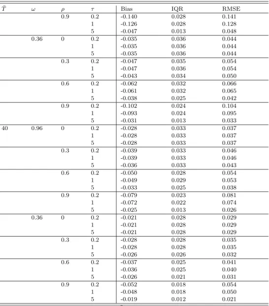
0.9 0.2 -0.140 0.028 0.141 1 -0.126 0.028 0.128 5 -0.047 0.013 0.048 0.36 0 0.2 -0.035 0.036 0.044 1 -0.035 0.036 0.044 5 -0.035 0.036 0.044 0.3 0.2 -0.047 0.035 0.054 1 -0.047 0.036 0.054 5 -0.043 0.034 0.050 0.6 0.2 -0.062 0.032 0.066 1 -0.061 0.032 0.065 5 -0.038 0.025 0.042 0.9 0.2 -0.102 0.024 0.104 1 -0.093 0.024 0.095 5 -0.031 0.013 0.033 40 0.96 0 0.2 -0.028 0.033 0.037 1 -0.028 0.033 0.037 5 -0.028 0.033 0.037 0.3 0.2 -0.039 0.033 0.046 1 -0.039 0.033 0.046 5 -0.036 0.033 0.043 0.6 0.2 -0.050 0.028 0.054 1 -0.049 0.029 0.053 5 -0.033 0.025 0.038 0.9 0.2 -0.079 0.023 0.081 1 -0.072 0.022 0.074 5 -0.025 0.013 0.026 0.36 0 0.2 -0.021 0.028 0.029 1 -0.021 0.028 0.029 5 -0.021 0.028 0.029 0.3 0.2 -0.028 0.028 0.035 1 -0.028 0.028 0.035 5 -0.026 0.026 0.032 0.6 0.2 -0.037 0.025 0.041 1 -0.036 0.025 0.040 5 -0.026 0.021 0.031 0.9 0.2 -0.052 0.018 0.054 1 -0.048 0.018 0.050 5 -0.019 0.012 0.021
Table 3: MSE of the Predictors
¯
T ω ρ τ OLS FE RE FEAR REAR
5 0.96 0 0.2 1 5 20.062 20.062 20.062 11.659 11.659 11.659 11.455 11.455 11.455 12.040 12.040 12.040 11.977 11.977 11.977 0.3 0.2 1 5 21.034 21.036 21.070 12.393 12.445 13.773 12.101 12.142 13.120 12.405 12.433 13.194 12.102 12.116 12.525 0.6 0.2 1 5 25.578 25.602 26.237 14.827 15.484 31.991 14.490 15.029 27.997 13.083 13.341 18.936 12.533 12.663 15.547 0.9 0.2 1 5 50.502 61.731 346.585 19.448 22.006 85.625 19.692 21.678 82.645 14.132 15.226 36.620 14.242 14.428 21.583 0.36 0 0.2 1 5 19.712 19.712 19.712 11.113 11.113 11.113 10.988 10.988 10.988 11.282 11.282 11.282 11.200 11.200 11.200 0.3 0.2 1 5 20.734 20.737 20.784 12.006 12.035 12.677 11.823 11.847 12.360 11.437 11.452 11.780 11.201 11.213 11.468 0.6 0.2 1 5 25.418 25.437 25.871 15.550 15.942 25.493 15.263 15.594 23.210 11.863 11.948 13.917 11.344 11.391 12.439 0.9 0.2 1 5 56.347 62.653 215.656 24.022 27.480 114.272 24.166 27.108 110.148 12.756 13.492 26.889 12.712 12.661 15.170 10 0.96 0 0.2 1 5 20.011 20.011 20.011 10.855 10.855 10.855 10.799 10.799 10.799 10.960 10.960 10.960 10.922 10.922 10.922 0.3 0.2 1 5 20.986 20.987 21.041 11.815 11.835 12.241 11.714 11.731 12.079 11.036 11.046 11.251 10.902 10.912 11.109 0.6 0.2 1 5 25.539 25.558 26.005 15.831 16.096 22.184 15.619 15.849 20.820 11.279 11.324 12.364 10.932 10.966 11.637 0.9 0.2 1 5 58.684 61.969 146.389 27.884 32.137 135.067 27.929 31.712 129.994 12.043 12.571 21.495 11.925 11.840 13.263 0.36 0 0.2 1 5 20.064 20.064 20.064 10.603 10.603 10.603 10.583 10.583 10.583 10.646 10.646 10.646 10.632 10.632 10.632 0.3 0.2 1 5 21.009 21.011 21.039 11.558 11.563 11.722 11.513 11.518 11.660 10.672 10.675 10.756 10.617 10.620 10.714 0.6 0.2 1 5 25.491 25.500 25.668 15.911 16.008 18.610 15.780 15.865 18.056 10.770 10.782 11.194 10.611 10.623 10.980 0.9 0.2 1 5 60.888 61.863 86.469 33.890 38.042 142.262 33.795 37.594 136.592 11.311 11.524 15.610 11.128 11.033 11.583 20 0.96 0 0.2 1 5 19.827 19.827 19.827 10.441 10.441 10.441 10.425 10.425 10.425 10.461 10.461 10.461 10.447 10.447 10.447 0.3 0.2 1 5 20.780 20.780 20.786 11.385 11.389 11.483 11.354 11.358 11.443 10.472 10.474 10.522 10.435 10.438 10.497 0.6 0.2 1 5 25.374 25.376 25.426 15.910 15.974 17.472 15.818 15.875 17.172 10.519 10.530 10.769 10.431 10.442 10.682 Continued on Next Page. . .
Table 3 – Continued ¯
T ω ρ τ OLS FE RE FEAR REAR
0.9 0.2 1 5 61.796 62.118 69.479 38.709 42.446 135.669 38.521 41.993 130.267 10.912 11.025 13.214 10.706 10.642 10.911 0.36 0 0.2 1 5 19.978 19.978 19.978 10.315 10.315 10.315 10.308 10.308 10.308 10.248 10.248 10.248 10.246 10.246 10.246 0.3 0.2 1 5 20.986 20.987 20.990 11.553 11.557 11.624 11.531 11.535 11.598 10.264 10.267 10.292 10.256 10.259 10.292 0.6 0.2 1 5 25.703 25.705 25.740 17.024 17.071 18.133 16.937 16.979 17.931 10.305 10.312 10.415 10.288 10.297 10.426 0.9 0.2 1 5 62.733 62.795 64.331 53.855 57.725 152.980 53.356 57.037 148.293 10.632 10.671 11.526 10.423 10.382 10.452 40 0.96 0 0.2 1 5 20.068 20.068 20.068 10.235 10.235 10.235 10.228 10.228 10.228 10.213 10.213 10.213 10.210 10.210 10.210 0.3 0.2 1 5 21.109 21.109 21.110 11.455 11.458 11.513 11.436 11.439 11.492 10.222 10.222 10.232 10.214 10.215 10.229 0.6 0.2 1 5 25.902 25.904 25.927 16.942 16.980 17.883 16.874 16.909 17.741 10.245 10.247 10.297 10.248 10.252 10.323 0.9 0.2 1 5 64.074 64.126 65.161 59.933 63.567 154.393 59.390 62.883 150.596 10.469 10.467 10.850 10.331 10.298 10.304 0.36 0 0.2 1 5 20.303 20.303 20.303 10.306 10.306 10.306 10.302 10.302 10.302 10.255 10.255 10.255 10.256 10.256 10.256 0.3 0.2 1 5 21.371 21.371 21.371 11.531 11.533 11.581 11.520 11.522 11.569 10.260 10.259 10.261 10.269 10.269 10.273 0.6 0.2 1 5 26.151 26.150 26.158 17.054 17.089 17.906 17.009 17.042 17.815 10.277 10.276 10.290 10.324 10.323 10.350 0.9 0.2 1 5 63.944 63.965 64.759 63.308 66.720 151.605 62.798 66.107 148.949 10.403 10.397 10.533 10.323 10.304 10.289 Note:N= 50 for all experiments.τ /(1−ρ2) is the variance of the initial condition.
Table 4: MAE of the Predictors
¯
T ω ρ τ OLS FE RE FEAR REAR
5 0.96 0 0.2 1 5 3.576 3.576 3.576 2.728 2.728 2.728 2.703 2.703 2.703 2.770 2.770 2.770 2.761 2.761 2.761 0.3 0.2 1 5 3.660 3.660 3.663 2.809 2.815 2.964 2.775 2.781 2.892 2.810 2.814 2.900 2.774 2.777 2.824 0.6 0.2 1 5 4.030 4.032 4.083 3.070 3.140 4.516 3.035 3.093 4.224 2.884 2.915 3.473 2.823 2.839 3.146 0.9 0.2 1 5 5.666 6.268 14.855 3.515 3.738 7.384 3.537 3.710 7.254 2.996 3.111 4.836 3.009 3.028 3.711 0.36 0 0.2 1 5 3.548 3.548 3.548 2.659 2.659 2.659 2.644 2.644 2.644 2.680 2.680 2.680 2.669 2.669 2.669 0.3 0.2 1 5 3.641 3.641 3.646 2.766 2.769 2.841 2.745 2.748 2.805 2.698 2.700 2.737 2.670 2.671 2.699 0.6 0.2 1 5 4.031 4.032 4.066 3.146 3.184 4.028 3.117 3.150 3.843 2.750 2.758 2.973 2.689 2.694 2.809 0.9 0.2 1 5 5.996 6.317 11.710 3.919 4.183 8.532 3.931 4.156 8.376 2.853 2.930 4.139 2.850 2.841 3.104 10 0.96 0 0.2 1 5 3.569 3.569 3.569 2.634 2.634 2.634 2.627 2.627 2.627 2.646 2.646 2.646 2.641 2.641 2.641 0.3 0.2 1 5 3.652 3.652 3.656 2.745 2.747 2.791 2.734 2.735 2.773 2.655 2.656 2.678 2.638 2.639 2.661 0.6 0.2 1 5 4.032 4.034 4.070 3.178 3.202 3.752 3.157 3.178 3.637 2.682 2.687 2.803 2.641 2.644 2.720 0.9 0.2 1 5 6.098 6.269 9.642 4.216 4.522 9.266 4.219 4.493 9.090 2.771 2.828 3.698 2.758 2.747 2.903 0.36 0 0.2 1 5 3.570 3.570 3.570 2.589 2.589 2.589 2.586 2.586 2.586 2.593 2.593 2.593 2.591 2.591 2.591 0.3 0.2 1 5 3.650 3.650 3.653 2.703 2.704 2.724 2.697 2.698 2.716 2.597 2.597 2.608 2.589 2.590 2.603 0.6 0.2 1 5 4.025 4.025 4.038 3.176 3.187 3.441 3.163 3.173 3.389 2.609 2.612 2.665 2.589 2.591 2.638 0.9 0.2 1 5 6.230 6.281 7.417 4.634 4.912 9.508 4.627 4.882 9.317 2.678 2.704 3.154 2.657 2.646 2.713 20 0.96 0 0.2 1 5 3.559 3.559 3.559 2.579 2.579 2.579 2.577 2.577 2.577 2.582 2.582 2.582 2.580 2.580 2.580 0.3 0.2 1 5 3.642 3.642 3.642 2.691 2.692 2.703 2.688 2.688 2.698 2.583 2.583 2.589 2.578 2.578 2.585 0.6 0.2 1 5 4.027 4.027 4.031 3.184 3.190 3.336 3.174 3.180 3.307 2.589 2.590 2.619 2.577 2.579 2.608 Continued on Next Page. . .
Table 4 – Continued ¯
T ω ρ τ OLS FE RE FEAR REAR
0.9 0.2 1 5 6.268 6.282 6.641 4.976 5.206 9.297 4.964 5.179 9.109 2.635 2.648 2.900 2.612 2.603 2.634 0.36 0 0.2 1 5 3.560 3.560 3.560 2.557 2.557 2.557 2.556 2.556 2.556 2.547 2.547 2.547 2.546 2.546 2.546 0.3 0.2 1 5 3.651 3.651 3.651 2.703 2.703 2.710 2.701 2.701 2.708 2.548 2.548 2.550 2.547 2.547 2.550 0.6 0.2 1 5 4.042 4.042 4.045 3.283 3.288 3.389 3.275 3.279 3.371 2.552 2.553 2.564 2.550 2.551 2.565 0.9 0.2 1 5 6.304 6.308 6.387 5.818 6.021 9.755 5.793 5.987 9.605 2.594 2.598 2.698 2.568 2.563 2.568 40 0.96 0 0.2 1 5 3.571 3.571 3.571 2.552 2.552 2.552 2.551 2.551 2.551 2.549 2.549 2.549 2.549 2.549 2.549 0.3 0.2 1 5 3.661 3.661 3.661 2.699 2.699 2.706 2.696 2.697 2.703 2.550 2.550 2.551 2.549 2.549 2.551 0.6 0.2 1 5 4.053 4.053 4.055 3.279 3.282 3.368 3.272 3.275 3.354 2.553 2.553 2.559 2.553 2.553 2.562 0.9 0.2 1 5 6.384 6.386 6.437 6.144 6.324 9.697 6.117 6.292 9.580 2.581 2.581 2.626 2.562 2.558 2.560 0.36 0 0.2 1 5 3.594 3.594 3.594 2.561 2.561 2.561 2.561 2.561 2.561 2.555 2.555 2.555 2.555 2.555 2.555 0.3 0.2 1 5 3.688 3.687 3.687 2.706 2.706 2.712 2.705 2.705 2.710 2.556 2.556 2.556 2.557 2.557 2.557 0.6 0.2 1 5 4.078 4.078 4.079 3.293 3.297 3.374 3.289 3.292 3.366 2.558 2.558 2.560 2.565 2.565 2.568 0.9 0.2 1 5 6.390 6.391 6.432 6.324 6.482 9.457 6.300 6.454 9.380 2.575 2.574 2.589 2.566 2.564 2.561 Note: N= 50 for all experiments.τ /(1−ρ2) is the variance of the initial condition.
Table 5: MAPE of the Predictors
¯
T ω ρ τ OLS FE RE FEAR REAR
5 0.96 0 0.2 1 5 388.781 388.781 388.781 364.873 364.873 364.873 347.241 347.241 347.241 374.599 374.599 374.599 361.344 361.344 361.344 0.3 0.2 1 5 472.399 543.080 408.194 394.322 424.699 400.761 370.196 395.002 366.890 395.632 427.752 390.466 367.692 393.979 351.306 0.6 0.2 1 5 371.881 352.733 675.286 410.321 395.485 1471.764 386.695 367.156 1307.010 385.988 369.172 1020.926 351.848 328.525 795.121 0.9 0.2 1 5 271.515 241.323 221.586 287.700 311.349 297.925 276.200 303.178 295.588 256.298 265.039 199.071 232.382 242.539 175.240 0.36 0 0.2 1 5 568.493 568.493 568.493 511.893 511.893 511.893 500.355 500.355 500.355 526.548 526.548 526.548 519.162 519.162 519.162 0.3 0.2 1 5 663.620 635.870 578.635 504.944 491.649 473.317 472.328 461.389 441.880 520.457 500.913 473.201 477.871 461.624 433.509 0.6 0.2 1 5 436.830 323.176 343.554 340.231 302.449 452.999 331.524 290.554 420.084 321.295 282.579 338.357 304.499 262.214 302.176 0.9 0.2 1 5 536.172 339.431 296.403 573.998 362.950 638.546 557.402 353.319 631.597 373.336 267.107 326.427 307.967 245.592 266.351 10 0.96 0 0.2 1 5 507.105 507.105 507.105 331.547 331.547 331.547 328.826 328.826 328.826 334.001 334.001 334.001 331.750 331.750 331.750 0.3 0.2 1 5 419.093 419.633 422.457 303.235 303.216 308.346 296.054 296.009 299.043 293.198 293.091 295.611 282.471 282.448 283.320 0.6 0.2 1 5 477.066 403.383 470.734 391.849 382.440 564.990 385.872 374.101 534.902 330.971 316.133 406.885 317.429 297.884 361.299 0.9 0.2 1 5 394.535 657.131 363.493 332.292 608.006 757.189 327.953 600.628 744.736 244.422 460.184 280.140 238.606 432.760 217.670 0.36 0 0.2 1 5 515.523 515.523 515.523 308.034 308.034 308.034 308.532 308.532 308.532 303.731 303.731 303.731 306.309 306.309 306.309 0.3 0.2 1 5 820.423 817.758 804.463 579.910 576.675 561.687 584.989 581.895 568.271 486.742 481.931 456.013 488.252 483.171 456.192 0.6 0.2 1 5 541.557 543.008 664.811 407.318 404.685 561.389 408.491 406.128 561.359 319.719 316.472 429.551 315.776 313.995 430.648 0.9 0.2 1 5 478.897 498.468 671.631 352.948 332.856 1023.864 344.789 320.943 1006.655 204.472 190.843 323.556 208.310 205.824 288.608 20 0.96 0 0.2 1 5 735.155 735.155 735.155 606.707 606.707 606.707 604.971 604.971 604.971 605.472 605.472 605.472 603.203 603.203 603.203 0.3 0.2 1 5 747.760 747.064 743.592 503.655 502.110 495.168 510.359 509.011 503.430 495.780 494.440 487.975 509.192 507.842 502.421 0.6 0.2 1 5 620.470 623.924 644.380 448.076 455.387 502.154 453.185 460.378 506.337 354.475 358.678 381.293 360.875 365.064 386.356 Continued on Next Page. . .
Table 5 – Continued ¯
T ω ρ τ OLS FE RE FEAR REAR
0.9 0.2 1 5 572.536 441.088 534.917 494.404 360.780 998.425 491.723 355.768 978.935 258.131 203.415 278.228 253.562 197.831 242.891 0.36 0 0.2 1 5 448.128 448.128 448.128 275.879 275.879 275.879 280.058 280.058 280.058 175.659 175.659 175.659 177.954 177.954 177.954 0.3 0.2 1 5 276.183 276.175 276.135 157.497 157.306 156.461 160.107 159.923 159.268 150.674 150.743 150.758 156.668 156.723 156.956 0.6 0.2 1 5 585.028 584.386 581.580 277.583 280.559 297.120 275.941 278.667 293.132 249.051 251.681 265.511 232.881 235.231 245.963 0.9 0.2 1 5 519.122 469.154 690.008 461.106 388.893 612.667 459.089 388.020 600.099 171.033 127.027 279.444 164.562 126.163 300.555 40 0.96 0 0.2 1 5 132.745 132.745 132.745 73.487 73.487 73.487 74.413 74.413 74.413 72.354 72.354 72.354 73.275 73.275 73.275 0.3 0.2 1 5 195.023 195.025 195.035 106.445 106.565 107.217 107.825 107.949 108.691 90.899 90.968 91.289 94.947 95.043 95.617 0.6 0.2 1 5 206.088 206.086 206.090 134.901 135.425 138.809 136.284 136.810 140.421 98.269 98.373 98.532 103.515 103.656 104.194 0.9 0.2 1 5 434.826 660.541 488.213 338.220 571.856 618.274 339.467 570.239 612.791 125.598 237.506 111.589 127.396 231.242 111.776 0.36 0 0.2 1 5 35.574 35.574 35.574 22.870 22.870 22.870 22.934 22.934 22.934 22.393 22.393 22.393 22.445 22.445 22.445 0.3 0.2 1 5 35.348 35.348 35.350 24.015 24.015 24.047 24.068 24.068 24.101 22.729 22.726 22.714 22.919 22.916 22.908 0.6 0.2 1 5 49.704 49.697 49.672 36.403 36.458 37.131 36.511 36.565 37.237 25.224 25.215 25.147 25.842 25.838 25.813 0.9 0.2 1 5 502.623 435.106 840.215 527.477 415.868 902.339 526.176 415.743 900.909 69.947 104.319 112.293 73.859 114.070 118.572 Note:N= 50 for all experiments. τ /(1−ρ2) is the variance of the initial condition.
Table 6: Estimation and Forecasting Results using the National Longitudinal Study
OLS FE RE FEAR REAR
age 0.0405 0.0417 0.0414 0.0420 0.0415 (0.0037) (0.0033) (0.0031) (0.0031) (0.0032) age2 -0.0007 -0.0009 -0.0008 -0.0009 -0.0008 (0.0001) (0.0001) (0.0001) (0.0001) (0.0001) exp 0.0271 0.0398 0.0348 0.0399 0.0347 (0.0011) (0.0017) (0.0013) (0.0016) (0.0013) tenure 0.0450 0.0334 0.0363 0.0332 0.0363 (0.0020) (0.0018) (0.0017) (0.0017) (0.0018) tenure2 -0.0018 -0.0020 -0.0019 -0.0020 -0.0019 (0.0001) (0.0001) (0.0001) (0.0001) (0.0001) nsmsa -0.1642 -0.0815 -0.1246 -0.0791 -0.1249 (0.0054) (0.0100) (0.0075) (0.0092) (0.0074) south -0.1007 -0.0501 -0.0833 -0.0475 -0.0830 (0.0052) (0.0116) (0.0077) (0.0107) (0.0076) grade 0.0622 0.0643 0.0643 (0.0011) (0.0019) (0.0019) black -0.0697 -0.0545 -0.0548 (0.0056) (0.0103) (0.0102) Intercept 0.2248 0.1822 0.1782 (0.0520) (0.0498) (0.0504) σµ 0.3245 0.2373 0.2684 0.2308 σv 0.3594 0.2732 0.2732 0.2747 0.2721 ρ 0.1012 0.1012 LBI 1.8404 1.8404 F-statistics 107.4471 107.4471 p-value 0.0000 0.0000 MSE 0.2136 0.1647 0.1610 0.1603 0.1559 MAE 0.3328 0.2688 0.2674 0.2623 0.2609 MAPE 41.1100 31.0870 32.3895 30.6727 32.2694
Note: The sample is an unbalanced panel data of 3640 women over the years 1968-1988 with gaps. We
compute the forecasts of logarithm wage for the last available year. In-sample model coefficient
estimates are based on 22887 observations from all previous years. For the in-sample, the average ¯
available yearsT = 6.288 and the Ahrens and Pincus indexω= 0.724. On average, we are forecasting ¯
S= 2.131 years ahead. MSE, MAE and MAPE are out-of-sample forecast comparison for the last
available year. σµ andσv are the standard deviations of the individual effects and remainder
disturbances, respectively. ρis the autocorrelation parameter of the remainder disturbances. LBI is the
locally best invariant test statistic in Baltagi and Wu (1999). F-statistics and p-value are for the panel
Table 7: Panel Data Test Results of Equal Predictive Accuracy using the National Lon-gitudinal Study
OLS FE RE FEAR REAR
OLS
FE -10.9947
RE -14.4038 -3.8038
FEAR -11.8924 -11.6062 -0.6650
REAR -16.2446 -6.9276 -10.5975 -3.5953
Note: The test statistic asymptotically follows a standard normal distribution. A negative entry
Appendix
Proof of Theorem 1
Proof. Denote T (1) as the set of observations when both ti,j and ti,j−1 are observed.
Equation (21) could be rewritten as ˆ
ρ= 1
m N
i=1 ti,j∈T(1)νˆi,ti,jνˆi,ti,j−1
1 n PN i=1 Pni j=1νˆi,t2 i,j . P P where ˜ − ˆ
νˆi,ti,j =yi,ti,j βF Ex˜i,ti,j =v˜i,ti,j − βˆF E−β x˜i,ti,j,
P
with y˜i,ti,j =yi,ti,j −y¯
−
i. and y¯i. =ni 1 nj=1i yi,ti,j. Other terms such as x˜i,ti,j, x¯i.,v˜i,ti,j and
v¯i. are similarly defined. Hence,
ˆ ρ−ρ = 1 m N
i=1 ti,j∈T(1)νˆi,ti,jνˆi,ti,j−1
1 n PN i=1 Pni j=1νˆi,t2 i,j −ρ = 1 m PN i=1 P
ti,j∈T(1) νˆi,ti,j −ρνˆi,ti,j−1
ˆ νi,ti,j−1 1 n PN i=1 Pni j=1νˆ 2 i,ti,j +ρ 1 m PN i=1 P ti,j∈T(1)νˆ 2 i,ti,j−1 − 1 n PN i=1 Pni j=1νˆ 2 i,ti,j 1 n PN i=1 Pni j=1νˆ 2 i,ti,j ! , P P
First of all, we have 1 n N X i=1 ni X j=1 ˆ νi,t2 i,j = 1 n N X i=1 ni X j=1 h ˜ vi,ti,j − ˆ βF E−β ˜ xi,ti,j i = 1 n N X i=1 ni X j=1 ˜ vi,t2 i,j + 1 n h√ nβˆF E−β i2 1 n N X i=1 ni X j=1 ˜ x2i,t i,j −2 n h√ n ˆ βF E −β i 1 √ n N X i=1 ni X j=1 ˜
vi,ti,jx˜i,ti,j
Following Lemma 7 in Hahn and Kuersteiner (2002), we can show 1 N ni
i=1 j=1v˜2
n i,ti,j =
σ2
that 1 P
+o N P
(1). Similarly, we can show ni 2 Pni
2 p i=1 j=1x˜i,ti,j =Op(1), 1 PN √ i=1 j=1v˜ x˜ = (1−ρ) i,t n n i,j i,ti,j
√ ˆ
Op(1) and n βF E −β =Op(1) under the assumptions stated in the Theorem. Hence
P P 1 n N X i=1 ni X j=1 ˆ νi,t2 i,j = σ 2 (1−ρ)2 +Op 1 n .
Similarly, we can show that 1 m N X i=1 X ti,j∈T(1) ˆ νi,t2i,j−1 = σ 2 (1−ρ)2 +Op 1 m . so that 1 m N X i=1 X ti,j∈T(1) ˆ νi,t2 i,j−1 − 1 n N X i=1 ni X j=1 ˆ νi,t2 i,j =Op 1 m −Op 1 n =Op 1 m . Also, we have ˆ
νi,ti,j −ρνˆi,ti,j−1
= hv˜i,ti,j − ˆ βF E −β ˜ xi,ti,j i −ρh˜vi,ti,j−1 − ˆ βF E −β ˜ xi,ti,j−1 i
= ˜vi,ti,j −ρ˜vi,ti,j−1
−βˆF E −β
˜
xi,ti,j −ρx˜i,ti,j−1
= ˜i,ti,j − ˆ βF E−β ˜
xi,ti,j −ρx˜i,ti,j−1
,
P
where ˜i,ti,j =i,ti,j −¯i.. with ¯
−
i.=n 1 ni
i j=1i,ti,j. Hence 1 m N X i=1 X ti,j∈T(1) ˆ
νi,ti,j −ρνˆi,ti,j−1
ˆ νi,ti,j−1 = 1 m N X i=1 X ti,j∈T(1) h ˜ i,ti,j − ˆ βF E−β ˜
xi,ti,j −ρx˜i,ti,j−1
i h ˜ vi,ti,j−1 − ˆ βF E−β ˜ xi,ti,j−1 i = N m 1 N N X i=1 X ti,j∈T(1) ˜
i,ti,jv˜i,ti,j−1
−√1 nm h√ n ˆ βF E−β i 1 √ m N X i=1 X ti,j∈T(1) ˜
vi,ti,j−1 x˜i,ti,j −ρx˜i,ti,j−1
−√1 nm h√ nβˆF E−β i 1 √ m N X i=1 X ti,j∈T(1) ˜
i,ti,jx˜i,ti,j−1
+1 n h√ nβˆF E −β i2 1 m N X i=1 X ti,j∈T(1) ˜
xi,ti,j −ρx˜i,ti,j−1
˜
xi,ti,j−1
Following Lemma 6 in Hahn and Kuersteiner (2002), we can showN1 Ni=1 ti,j∈T(1)˜i,ti,jv˜i,ti,j−1 =
σ2
+o (1). Similarly, we can show that √1 PN P
−ρ p m i=1 t ∈T(1)v˜i,t
1 i,j i,j−1 x˜i,ti,j −ρx˜i,ti,j−1 =
P Op(1), 1 N P N P 1 P √ − m i=1
t ∈T(1)˜i,ti,jx˜i,ti,j−1 =Op(1),
∈ x
m i=1 t T(1) ˜i,ti,j ρx˜i,ti,j−1 x˜i,ti,j−1 =
i,j i,j
√ ˆ
Op(1) and n βF E −β =Op(1) under the assumptions stated in the Theorem. Hence
1 m N X i Therefore, we have =1 X ti,j∈T(1) ˆ
νi,ti,j −ρνˆi,ti,j−1
ˆ νi,ti,j−1 =Op N m 1 N i=1 t ∈T(1) νˆ i,j−1 νˆ P P
i,ti,j −ρνˆi,t i,t
m i,j−1 ρˆ−ρ = i,j 1 N ni νˆ2 n P i=1 j=1 i,ti,j 1 PN 2 1 PN Pn ! − i 2 m i=1 ti,j∈T(1)νˆi,t νˆ ρ i,j−1 n i=1 j=1 i,t + i,j 1 PN Pni νˆ2 n i=1 j=1 i,ti,j N 1 N = Op +Op =Op . m m m P P