TI 2012-025/4
Tinbergen Institute Discussion Paper
Evidence on Features of a DSGE Business
Cycle Model from Bayesian Model
Averaging
Rodney Strachan
1Herman K. van Dijk
21 Research School of Economics, The Australian National University;
2 Econometric and Tinbergen Institutes, Erasmus University Rotterdam, and VU University Amsterdam.
Tinbergen Institute is the graduate school and research institute in economics of Erasmus University Rotterdam, the University of Amsterdam and VU University Amsterdam.
More TI discussion papers can be downloaded at http://www.tinbergen.nl
Tinbergen Institute has two locations: Tinbergen Institute Amsterdam Gustav Mahlerplein 117 1082 MS Amsterdam The Netherlands Tel.: +31(0)20 525 1600 Tinbergen Institute Rotterdam Burg. Oudlaan 50
3062 PA Rotterdam The Netherlands Tel.: +31(0)10 408 8900 Fax: +31(0)10 408 9031
Duisenberg school of finance is a collaboration of the Dutch financial sector and universities, with the ambition to support innovative research and offer top quality academic education in core areas of finance.
DSF research papers can be downloaded at: http://www.dsf.nl/
Duisenberg school of finance Gustav Mahlerplein 117 1082 MS Amsterdam The Netherlands Tel.: +31(0)20 525 8579
Evidence on Features of a DSGE Business Cycle model from
Bayesian Model Averaging
1;2Rodney W. Strachan
Research School of Economics, The Australian National University Herman K. van Dijk
Econometric and Tinbergen Institutes, Erasmus University Rotterdam and VU University Amsterdam
ABSTRACT
The empirical support for features of a Dynamic Stochastic General Equilibrium model with two technology shocks is evaluated using Bayesian model averaging over vector autoregressions. The model features include equilibria, restrictions on long-run
1*Manuscript received October 2008; revised September 2010.
2We would like to thank Frank Schorfheide and three anonymous referees for extensive comments
which led to a substantial revision and extension of the results presented in the original working paper. A preliminary version of this paper has been presented at the US Federal Reserve Bank in 2008 and at Cambridge University in 2011. We also thank Luc Bauwens, Geert Dhaene, John Geweke, David Hendry, Lennart Hoogerheide, Soren Johansen, Helmut Lutkepohl, Christopher Sims, Mattias Villani and Anders Warne for helpful discussions on the topic of this paper. Of course, any remaining errors remain the responsibility of the authors. Van Dijk acknowledges …nancial support from the Netherlands Organization of Scienti…c Research.
responses, a structural break of unknown date and a range of lags and deterministic processes. We …nd support for a number of features implied by the economic model and the evidence suggests a break in the entire model structure around 1984 after which technology shocks appear to account for all stochastic trends. Business cy-cle volatility seems more due to investment speci…c technology shocks than neutral technology shocks.
Key Words: Posterior probability; Dynamic stochastic general equilibrium model; Cointegration; Model averaging; Stochastic trend; Impulse response; Vector autoregressive model.
JEL Codes: C11, C32, C52
1 Introduction.
In this paper we evaluate the robustness, in face of model uncertainty, of the empir-ical support for long-run equilibrium relationships implied by a Dynamic Stochastic General Equilibrium (DSGE) business cycle model subject to a investment-speci…c technology shock and a neutral technology shock. We embed these features of the DSGE model within a set of Vector AutoRegressive (VAR) models and take into ac-count model uncertainty using a Bayesian Model Averaging (BMA) approach. Our work is distinguished from most other model averaging papers since averaging over systems of variables (rather that single equation models) implies averaging over fea-tures of the model rather than averaging over sets of regressors. Averaging over model features in systems of variables adds a level of complexity compared to single equation models and requires careful consideration of prior distributions. However, the approach we propose makes such an exercise feasible and the empirical results suggest the exercise is worthwhile.
The DSGE model investigated in this paper is based upon one described by Fisher (2006). This model has several features that can be empirically weighted: for exam-ple, the economic model suggests that the Great Ratios (e.g., consumption to income, investment to income) are stationary, that only investment-speci…c technology shocks have permanent e¤ects on the real investment good price, and only technology shocks a¤ect productivity in the long run. Model uncertainty derives from uncertainty over
the number of stochastic trends, on the form of the reduced form equilibrium (cointe-grating) relations, on the form of the deterministic trends, and, …nally, on lag length. By considering the unconditional evidence, where ‘unconditional’means that the em-pirical evidence does not depend upon a single model, it is possible to identify those features that have stronger empirical support. The joint evidence for those features implied by the model will indicate its empirical support.3
The idea underlying BMA is relatively straightforward. Model speci…c estimates are weighted by the corresponding posterior model probability and then averaged over the set of models considered. Although many statistical arguments have been made in the literature to support model averaging (e.g., Leamer 1978, Hodges 1987, Draper 1995, Min and Zellner 1993 and Raftery, Madigan and Hoeting 1997), an increasing number of recent applications suggest its relevance for macroeconometrics (Fernández, Ley and Steel 2001, Sala-i-Martin, Doppelho¤er and Miller 2004, Koop and Potter 2003, Wright 2008 and Koop, León-González and Strachan 2012). There are several arguments for model averaging and only a few are mentioned here. At the simplest level, it is often attractive to report inferences robust to model speci…cation. Second, a large body of applied work has demonstrated that averaging results in gains in forecasting accuracy (Bates and Granger 1969, Diebold and Lopez 1996,
3We use the word ‘features’rather than ‘structures’to avoid confusing our work with structural
Newbold and Harvey 2001, Terui and van Dijk 2002, Hoogerheide, Kleijn, Ravazzolo, van Dijk and Verbeek 2010 and Wright 2008). Some explanation for this phenomenon in particular cases was provided by Hendry and Clements (2002). Thirdly, from a methodological point of view, averaging over models addresses to some degree the well understood pre-test problem (see, for example, Poirier 1995, pp. 519-523).
There is clear evidence from the literature that a structural break should be con-sidered around 1984 (see, for example, McConnell and Perez-Quiros 2000 and Stock and Watson 2002). This literature suggests there is evidence of a break in possibly both the variances and mean equation coe¢ cients. There is little work to date on changes in the overall structure or features of the model, such as changes in lag dy-namics or stability of variables. We …nd the empirical evidence suggests that allowing for structural changes in the models, that is allowing the process to switch from one model to another, rather than just the parameter values, is justi…ed.4 Incorporating
this model switching is a computationally challenging task. We simplify this task by considering what was the most likely model before the break and which was the most likely model after the break, rather than trying to compute the evidence of the switch from one model structure to another.
This paper makes three contributions. First, we show how to obtain posterior
4The introduction of the structural break analysis was on the suggestion of a referee to whom we
inference from model averages in which the economically and econometrically impor-tant features may have weights other than zero or one. In other words, the inferences are based on a large …nite mixture of model structures. Second, this paper treats a structural break as a change in the entire structure of the model, not just a change in parameter values. We …nd strong evidence that the entire structure, rather than just the parameter values, has changed. This extension implies a very large model set but we demonstrate how to obtain inference using some simple algebra and fast computation. Third, the proposed methodology is demonstrated with an empirical investigation of the long-run equilibrium relationships implied by the DSGE model. Important in this model are the long run responses of investment prices and pro-ductivity to technology shocks and that technology follows stochastic rather than deterministic trends.
The structure of the paper is as follows. In Section 2 the important features of the economic model used by Fisher (2006) are outlined. In Section 3 the basic econometric models of interest in this paper are introduced, including characteriza-tions of the features implied by the economic model. We present priors, likelihood and the sampling scheme used in Section 4 together with the tools for inference in this paper including the posterior predictive probabilities (Geweke 1996 and Geweke and Amisano 2011) of alternative model features and the Laplace approximation. The posterior and predictive evidence of model features are presented in Section 5
as are estimates of important functions of parameters. In Section 6 we summarize conclusions and discuss possibilities for further research.
2 Long-Run Relations from a DSGE Business Cycle Model.
In this section we outline the features of a DSGE model that is based upon the real business cycle model of Fisher (2006), which is in turn based upon the competitive equilibrium growth model of Greenwood, Hercowitz, and Krusell (1997). We impose two simpli…cations: capital is not separated into equipment and structures; and tech-nologies are given stochastic rather than deterministic trends. The general model was developed in Kydland and Prescott (1982) and detailed in King, Plosser and Rebelo (1988), and an interesting early econometric analysis is provided in King, Plosser, Stock and Watson (1991, hereafter referred to as KPSW). The reader is directed to these papers for the development of the model as we focus upon certain features that imply restrictions upon our reduced form econometric model that we want to weight using BMA.
The model suggests that a system of consumption,Ct;investment,Xt;and output,
Yt=Ct+Xt;will share a balanced growth path since each is driven by shocks to two
technologies: an investment speci…c technology, Vt; and neutral technology, At. We
The resource constraint and Cobb-Douglas production technology are given by
Ct+Xt AtKtH
1
t ; 0< <1
and period t+ 1 capital stock is given by
Kt+1 (1 )Kt+VtXt; 0< <1:
Fisher (2006) speci…es technology as having stochastic rather than deterministic trends. The log of investment-speci…c technology, vt = ln (Vt);and the log of neutral
technology, at = ln (At);are assumed to be independent simple random walks,
possi-bly with drifts. In the empirical analysis we evaluate the evidence on the importance of deterministic and stochastic trends as well as the relative contribution to business cycle volatility of investment speci…c and neutral technology shocks.
The production technology and the resource constraint imply that we can repre-sent the log real price of an investment good in consumptions goods bypt= vt and
pt =pt 1 zI;t: Since 0; this is in accordance with the downward trend we
see in the price of an investment good. Neutral technology evolves by the process at= +at 1+zN;twhere 0and(zI;t; zN;t)0 has zero mean and constant covariance
matrix.
A …rst implication of this model is that the variables ct; xt; and yt will all be
integrated of order one due to a common stochastic trend given by !at+ (1 !)pt
in the balanced growth literature (see, for example, KPSW) and it implies that we can treat the Great Ratio relationsct ytand xt ytas valid cointegrating relations.
Denote by ht = ln (Ht) the log number of hours worked which is assumed to
have no unit root. Although it may have a trend over short periods, and the evidence suggests this, it is not possible for hours worked per capita to have a permanent trend. The log price of an investment good, pt; and labour productivity, at = ln (Yt=Ht) =
yt ht, are assumed to have unit roots but pt should not cointegrate with the other
variables. Sincehtis assumed to beI(0);andct;ytandxtare all assumed to beI(1)
sharing a common stochastic trend, the above assumptions imply thatatwill beI(1)
and ct yt and xt yt will be I(0). The assumptions of Fisher (2006) preclude the
above I(0) relations having deterministic trends and this is not a feature we would expect to …nd over long samples. By allowing for structural breaks we may …nd trends in one or more subsamples, perhaps as a trend in the second period o¤-sets the e¤ect of the trend in the …rst period, but we would expect that they are inherently temporary features.
Two important …nal restrictions apply. First, Fisher (2006) assumes that the long run response of pt to zI;t will be nonzero, in fact negative, but its long run response
to all other shocks will be zero. Second, the long run response of at to both zI;t
and zN;t will be nonzero, but the long run response of at to any other shock will be
the neutral technology shock, zN;t.
3 A Set of Vector Autoregressive Models.
When a VAR process cointegrates, the model may be written in the vector error correction model (VECM) form. The VECM of the 1 n vector time series process
yt = (pt; at; ht; ct; xt); t= 1; : : : ; T; conditioning on l+ 1 initial observations is
yt =yt 1 +dt + yt 1 1+: : :+ yt l l+"t (1)
where yt =yt yt 1: The 1 n vector of errors "t are assumed to be iidN(0; ).
The matrices j j = 1; : : : ; l aren n and and 0 aren r and assumed to have
rankr 2 f0;1; :::;5g: We de…ne the deterministic termsdt below.
As the model in the previous section implies two common stochastic trends, from the two technology shocks, there will be three cointegrating relations; that is r = 3. The model is quite speci…c about the form of these cointegrating relations and
these impose overidentifying restrictions on the cointegrating vectors. Speci…cally, the model says that: pt has a unit root but does not cointegrate with the other
variables in the system; that hours worked, ht, are stationary; and the great ratios
of consumption to income and investment to income, ct yt = ct at ht and
xt yt = xt at ht, are stationary. We index the overidentifying restrictions by
o and when all of the restrictions in the previous sentence are imposed we set o = 2 and this can only occur whenr = 3: When no restrictions are imposed we set o = 0
which can occur for anyrinf0;1; :::;5g:When we only impose the restriction thatpt
has a unit root but does not cointegrate then o= 1. The restrictiono = 1 is allowed to hold for1 r 4:
We allow for …ve lag lengths, l 2 f2;3;4;5;6g. The deterministic processes are denoted by d 2 f1;2;3;4;5g and these processes are the …ve most commonly used combinations of trends inyt and trends inyt (for details see Johansen 1995, Section
5.7). The two empirically important deterministic processes in this paper are d = 2 which implies a linear trend inyt and a linear drift inyt;andd= 4 which implies no
drift in the levels and no trend in the cointegrating relations. Some models implied by the deterministic processes will be observationally equivalent. For example, if
r = 0 then di¤erent models of trends in yt will be observationally equivalent. The
treatment of a priori impossible and observationally equivalent models is explained in the next section when the prior is outlined.
Finally, the long run restriction to identify the technology shocks is employed. As discussed in the previous subsection, this restriction implies that the long run response of pt is nonzero only for the investment-speci…c technology shocks and that
the long run response ofatis nonzero only for the investment-speci…c technology shock
and the neutral technology shocks. This restriction can be parameterized using the standard Beveridge-Nelson form of the Wold representation of the VECM as
The …rst two elements of zt = 1=2"t are the investment-speci…c technology shock,
zI;t, and the neutral technology shocks, zN;t, respectively. Further, = In li=1 i:
These restrictions imply the …rst two rows of C 1=2 will have the following zero
entries5: 2 6 6 4 0 0 0 0 0 3 7 7 5: (2)
This restriction is obtained by the appropriate choice of 1=2 such that = 1=2 1=20
andC 1=2has the structure shown above. For an explanation of how such restrictions
are implemented see the Appendix, and see Chang and Schorfheide (2003) and Del Negro and Schorfheide (2010) for further examples and discussion.
Since C has rank n r; and 1=2 must have rank n; the zero restrictions on
C 1=2 and the assumption of nonzero responses of pt and at stated above imply
C must have at least rank two, then this identi…cation scheme can only apply if
r 2 f0;1; : : : ; n 2g. This is consistent with the two technology shocks entering the system as stochastic trends.
Fisher (2006) assumes a break date around 1982 Q3, although our results suggest a slightly later date. We allow for a range of 16 break dates from the …rst quarter of 1982 until the last quarter of 1985. In our sample these periods cover the observations from t = 137 tot = 152: We index these dates by 2 f ; + 1; :::; + 15; g where the …rst break is at 1982Q1 ( = 137), the second break occurs at 1982Q2, and so on
until the last break at 1985Q4 ( = 152).
In total we average using255models before the structural break, and255after the break and twelve break dates. This gives a total of over 780;000 models that need to be computed. Computation of marginal likelihoods for this many multivariate models would be computationally challenging. As our interest is in the date when the break occurs and modelling after the break date, we need only estimate 510 marginal likelihoods for 12 break dates; a total of 6120 marginal likelihoods. This is still a large number of computations, but much more readily achievable. We provide further details on how this is achieved in Section 4.2.
4 Priors, Posteriors and Model Averaging.
In this section the priors and resultant posterior are presented. For notational con-venience we collect the lag parameters into a ki n matrix = [ 01 0l]
0 and
vectorize into = vec( ): Conditional upon ; the model in (1) is linear in the equation parameters , vec( ) and , while conditional upon , vec( ) and , the model is linear in : This fact makes it relatively straightforward to elicit priors on the parameters.
4.1 The Prior.
All models included for the averaging are treated equally likely. The set of models included for the averaging is a subset of the full set of models that result from all combinations ofr; o; dand l and 16 break dates . We exclude impossible and mean-ingless models and, if two or more models are observationally equivalent, we include only one of them. To avoid notational burden, and because we use the same prior for models before and after the structural break, in this section we do not distin-guish between parameters and models before and after the break dates except where necessary.
For we use a proper inverted Wishart prior with scale matrix S = In10 and
degrees of freedom = n+ 1 as this prior is rather uninformative. The parameters in are given a normal prior with zero mean and covariance matrix 1= V where
V = (Iu+V0(1 u)) (I(1 u) +V1u) and u 2 f0;1g with prior probabilities Pr (u= 1) = Pr (u= 0) = 0:5: Here V0 = Iki and V1 is the Litterman (1980,
1986) type prior for a VECM similar to that speci…ed in Villani (2001). We use a gamma prior with mean E( ) = 5 and a relatively large variance V ( ) = 16:67 for
: The settings we use provide a reasonable degree of shrinkage towards zero which has been shown to improve estimation (see Ni and Sun 2003).
We specify a weakly informative normal proper prior for vec( ; )0 conditional upon ( ; ; Mi) (and hyperparameters discussed below) with zero mean and
covari-ance matrix 1= Va where Va = Ir.6 Further details on the speci…cation of the
full prior is given at the end of the next subsection. The matrix is given a Normal prior with zero mean and covariance matrix n 1I
nr. The theory underpinning this
speci…cation is provided in Koop, León-González and Strachan (2010). Its motivation is to induce a uniform prior on the cointegrating space and a fast, e¢ cient sampling scheme.
Let a = vec( )0; vec( )0; 0 0; b= vec( ) and V be the block diagonal matrix withVaand V on the diagonals . Introduce as the vector containing the elements of ; a; and :The full prior distribution for the parameters in a given model is then
p( ; ; ujMi)_exp =2a0V 1a n=2b0b nnr=2
j j ( +n+1+r+uki)=2exp 1=2tr 1S n(ki+2r)+1exp
f 5 =6g:
Ideally all models would be treated as a priori equally likely, however this is not a straightforward issue in VECMs.7 The priors for the individual elements of
i = (r; o; d; l) are not independent, as certain combinations are either impossible (such as whenr=nando = 2), meaningless (such as, for example, r= 0witho = 1) or observationally equivalent to another combination (such as the models withr =n
6If an informative prior is used on for the cointegrating space then we recommend the prior for
described in Koop, León-González and Strachan (2008). Further details on the development of this prior are available in an earlier working paper version of this paper: Strachan and van Dijk (2010).
7The authors are grateful to Geert Dhaene, John Geweke and an anonymous referee for useful
and d = 1 or 2). The prior probability for impossible and meaningless models is set to zero. However, the researcher must carefully consider how she wishes to treat observationally equivalent models. Treating these models as just one model and then assigning equal prior probabilities to all models biases the prior weight in favour of models with 0< r < n: This could shift the posterior weight of evidence in favour of some economic theories for which we wish to determine the support.8 Alternatively,
these could be treated as separate models. A choice must be made and in this paper, observationally equivalent models are treated as one model.
A referee raised the interesting question as to whether it is appropriate to specify independent priors for r; o; d and l: One might expect, for example, that a strong deterministic process such as d = 1 might reduce the prior expectation of …nding stochastic trends in the processes. This might imply that the probabilityPr (r < njd) may decrease as d increases. Similarly a shorter lag length, l, might be associated with a higher prior probability of …nding (more) stochastic trends. We do not pursue this idea further, but note that it might be a worthwhile topic for investigation.
4.2 Posterior Analysis.
We conduct the empirical investigation in two stages. We …rst compute the esti-mated model probabilities and the timing of the structural break. We then estimate
8This issue could be viewed as a con‡ict between the desire to be uninformative across statistical
the functions of interest such as impulse responses and variance decompositions. We estimate the model probabilities using a Laplace approximation of predictive densi-ties, and the impulse responses and variance decompositions are estimated using a Gibbs sampler.
When investigating the evidence on structural breaks we encounter two issues that need to be addressed: the strength of the prior information; and proliferation of models to compute. As we have a separate prior for the parameters before and after the break, we have e¤ectively doubled the amount of prior information in the posterior and halved the amount of data (on average) used to estimate the parameters. This introduces the problem that the prior information is strong relative to the data. We could make the priors less informative, but then that increases their in‡uence in the computation of the posterior probabilities (see discussion on Bartlett’s paradox in Geweke 2005, Section 2.6.2). This situation implies a trade o¤ between prior uncertainty about the parameters and posterior uncertainty about the models. To mitigate this issue we compute predictive probabilities (see, for example, Geweke 1996 and Geweke and Amisano 2011) from predictive densities.
The predictive densities can be derived for each model via the expression
pT0;T2 i =p y T2 T1+1jy T1 T0; Mi = R p yT2 T1+1jy T1 T0; Mi; p y T1 T0jMi; p( jMi)d R p yT1 T0jMi; p( jMi)d (3) where = ( ; u; )and yt1
t0 is the data from observationt0 tot1:For a model prior to
a model after the structural break, T0 = and T2 =T: As T2 ! 1 orT1 !0; then
p yT2
T1+1jy
T1
T0; Mi becomes the standard marginal likelihood. Thus the full predictive
density for a process that switches from model Mi to model Mj at time is the
product pi =p1i; 1pj;T:
We estimate the numerator and denominator in (3), and therefore pT0;T2
i , using
the Laplace approximation. This technique approximates the integral by a second order expansion around the mode of the log of the integrand (see Tanner 1993). Although often described as a normal approximation, the Laplace approximation has been shown to work very well with many non-normal distributions. For example, Strachan and Inder (2004) apply the approach to the VECM where the integral is over linear subspaces which have bounded supports and non-standard distributions. Denoting by the set of models and using the notationpT0;T2; =
j2 p
T0;T2
j ;then at a
given break date we can compute the posterior predictive probability of a modelMi
holding before (or after) the break using the pT0;T2
i as p MijyTT20; =pTi0;T2 pT0;T2; .
While using the Laplace approximation greatly speeds up the computation of the model probabilities, as discussed earlier, we allow the entire model structure to change at the break. This implies we have a very large number of models because the process is allowed to switch from any model before the break to any model after the break. To further reduce computation time, we make use of the fact that we are only interested in computing the probability that a break occurs at a point in time,
and not which model after the break followed a speci…c model before the break. This observation greatly reduces the number of necessary computations.
If we have K possible break dates, then the posterior probability of a break at date = is obtained by p( = jy) = p1; 1; p ;T; = K
=1 p1; 1; p ;T; :
This expression, explained in a working paper (Strachan and van Dijk 2012), reduces the required number of computations from 780,300 to 6,120. The probability of a particular feature (e.g.,d = 2) holding after the break is then obtained by summing the products of the probabilities of the models with that feature and the probabilities of their break dates.
To estimate the impulse responses we require draws from the posteriors of the models with non-negligible posterior weight. An expression for the posterior distrib-ution of the parameters for any model given the data is obtained by combining the prior, p( ; ; ujMi); with the likelihood for the data L(yj ; Mi) where y represents
all data. That is,9 p( ; ; ujMi; y) _p( ; ; ujMi)L(yj ; Mi): As the sampler uses a
Gibbs sampling scheme, it is necessary to present the conditional posterior for each parameter.
In the following results, we gather together terms to keep expressions notationally concise. Collect yt 1 and the vector z2;t = (d2;t; yt 1; : : : ; yt l) into the vector
zt= (yt 1 ; z2;t)and recall the de…nition ofa = vec( )0; vec( )0; 0 0. As the model
is linear conditional upon b = vec( ); standard results show that the posterior for
a conditional on all other parameters will be normal with mean a and covariance matrix V constructed as a = V 1 Iki+r vec T t=1zt0 yt and V = 1 Tt=1zt0zt + V 1 1 :
Next, the posterior for b conditional upon the other parameters will be normal with mean b and covariance matrix Vb which are constructed as
b = Vb 1 In vec Tt=1y0t 1( yt z2;t )
and
Vb = 1 0 Tt=1yt0 1yt 1 +nInr
1
:
The posterior for will be Gamma with degrees of freedom =n(ki+r)+3and
mean = 1= a0V 1a+ 5=3 = (see, for example, Koop 2003): Finally, uwill have
a Bernoulli conditional posterior distribution withp= Pr (u= 1ja; ; ; y) equal to
p= exp =2a0V01a = exp =2a0V01a + exp =2a0V11a :
We use the following scheme at each step q to obtain draws of(a; ; ; ; u) :
2. Draw jb; a; ; ufromIW S+u A0A+PT
t=1"0t"t; T +uki+r ;
3. Draw aj ; b; ; u fromN a; V ;
4. Draw bj ; a; ; u fromN b; Vb ;
5. Draw j ; b; a; u from Gamma( ; );
6. Draw uj ; b; a; fromBernoulli(p);
7. Repeat steps 2 to 6 for a suitable number of replications.
To end this section we outline how we implement Bayesian model averaging. Let ( ; Mi) be an economic object of interest which is a function of the parameters, ,
for a given model,Mi. Examples include estimates of impulse responses, forecasts, or
loss functions. To report the unconditional (of parameters or any particular model) expectation of this object it is necessary to estimateE( jy) =
i2 E( jy; Mi)p(Mijy)
whereE( jy; Mi)is the expectation of ( ; Mi)from modelimarginal of :Estimate
E( jy; Mi)as follows. First denote theqthdraw of the parameters from the posterior
distribution for modelMi as (q)and so theqthdraw of ( ; Mi)as (q); Mi . Using
J draws of the parameters from the posterior distribution for each of the models in , obtain estimates of E( jy; Mi) from each model by Eb( jy; Mi) = J1 Jq=1 (q); Mi .
These estimates are then averaged as Eb( jy) =
i2 Eb( jy; Mi)pb(Mijy) in which
b
5 Evidence on Model Features.
In this section we provide empirical evidence on the support for the features of the DSGE model with two technology shocks and the various restrictions that this eco-nomic model implies for the econometric model. We begin with providing evidence on the timing of the structural break, and the posterior probabilities of the features of the reduced form VECM that are implied by this DSGE model. We estimate the posterior probability of a structural break occurring at a range of dates and, in sub-sequent analysis, focus upon the results for the data after the structural break. We then report the estimates of objects of interest including impulse response functions.
The variables and the data: The variables of interest are: log real price of an investment good measured in consumptions units, pt; log labour productivity, at;
log number of hours worked, ht; log of consumption,ct; and log investment, xt. The
data, which are seasonally adjusted, start in the …rst quarter of 1948 and end in the second quarter of 2009. Where appropriate, the data are measured in 1996 dollars de‡ated using a chain-weighted index of consumption prices. For more background on the data we refer to the working paper Strachan and Van Dijk (2012).
Break Dates and Stability of Great Ratios: Three break dates receive mea-surable support, 1984Q3, 1984Q4 and 1985Q1 with probabilities of 0.01%, 57.78% and 42.21% respectively. Of the 765 models over these three dates, there were 62 post break models with measurable support and 12 pre-break models with
measur-able support. From the pre-break models, the model with one cointegrating relation, no overidentifying restrictions, no drift and two lags, (r; o; d; l) = (1;0;4;2); with a break at 1984Q4 has 57.8% of the probability mass and the same model with with a break at 1985Q1 has 41.3% posterior probability. Thus, the models prior to the break provide strong evidence against the features we would expect under the eco-nomic model. While the results prior to 1984 have important information in them, there is evidence of several breaks in the 1970. As the aim of this paper is not a comprehensive treatment of all breaks, the remainder of the discussion focuses on the post break results as this period is well represented by a single, stable model.
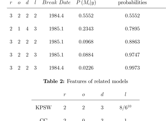
Among the post break models, one model accounted for half the posterior mass and the top …ve models accounted for 99.73% of the posterior probability mass, as presented in Table 1. The posterior probabilities of the top …ve models are presented in Table 1. Post the break, the model(3;2;2;2)with a break at 1984 Q4 and the model (2;1;4;3) with a break at 1985 Q1 capture 79% of the probability mass. Although relatively few models get any support, it is clear that support is fairly strong for the top …ve models.
As the primary aim of this paper is to investigate the degree and role of model uncertainty in the empirical evidence on technology shocks and important features of DSGE models, we discuss the results with reference to a number of important papers in the literature. In Table 2 we have summarized the relevant features of the model
by Fisher and compare this with results found in the literature in the KPSW study and the study by Centoni and Cubadda (2003, hereafter CC). We note that none of these speci…c models receive notable posterior support with our data set.
The posterior probability of having only two stochastic trends (r = 3) is 76%, although there is evidence of a third if the break is delayed until 1985 Q1. The DSGE model is driven by technology shocks which, in Fisher and KPSW, are stochastic trends. These are the only stochastic trends described in the economic model and KPSW assume a unique technology is (in the three variable model) the only stochastic trend that enters the system. The economic model of Fisher implies there are only two common stochastic trends. CC report evidence of an extra stochastic trend in a three variable system, but they then choose use the single trend model for inference. We conclude the evidence on an extra unit root is an empirical issue. It is possible the extra stochastic trend could be entering from the hours worked variable,ht. Whileht
does not display a trend, it does display a very large and slow cyclical component with peak-to-peak cycles of around 10 years duration and a sudden drop in 2009. Such large cycles and outliers are not easily captured in linear models (such as the VECM) and may be manifesting as evidence of a third unit root. An alternative explanation is provided in Chang, Doh and Schorfheide (2007), that hours may appear nonstationary if labour adjustment costs are not explicitly incorporated into the model.
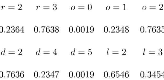
That is, there is a 76% probability that the Great Ratios are stable and that the investment price has a unit root and does not cointegrate with the other variables (o= 2). The assumptions that the price of an investment good is nonstationary and does not cointegrate with any other variable in the system, with 99% probability mass ono= 1 ando= 2, have very strong support. Since the joint posterior probability of (r= 3; o= 2) is 76%, and the posterior probability of(r = 3; o= 0 oro= 1) is zero, the evidence that the Great Ratios are stationary is positive, although not compelling. According to the model of Fisher, it might be reasonable to expect few determin-istic processes in the system and so to see d 3 as the technologies are commonly described as random walks possibly with drifts, but the economic model does not suggest we would expect trends in the cointegrating relations (d = 2) or quadratic trends in the variables (d = 1). Table 3 presents the marginal probabilities of the various features of the VECM. There is a 76% probability that there is a drift in the levels and a trend in the cointegrating relations (d = 2) and 24% probability of no drift in levels and no trend in the equilibria (d= 4). With a 76% posterior probability that the cointegrating relations are the Great Ratios of consumption to income and investment to income, the trend may be picking up the decline in the savings that occurred since the mid 1990s.
Overall the evidence in the estimated probabilities for the features of the econo-metric model suggested by the DSGE model of Fisher (2006) is positive to strong.
But, with 25% of the mass on features not supported by the economic model, the evidence is not decisive and there remains considerable model uncertainty.
Table 1: Posterior probabilities,P (Mijy), of the top …ve models.
Cumulative
r o d l Break Date P (Mijy) probabilities
3 2 2 2 1984:4 0:5552 0:5552
2 1 4 3 1985:1 0:2343 0:7895
3 2 2 2 1985:1 0:0968 0:8863
3 2 2 3 1985:1 0:0884 0:9747
3 2 2 3 1984:4 0:0226 0:9973
Table 2: Features of related models
r o d l
KPSW 2 2 3 8=610
CC 2 0 3 1
Fisher11 0 0 3 3
10KPSW use 6 lags when testing for cointegration but 8 lags to produce the variance
decomposi-tions. In our results labelled KPSW below, we average over 6 to 8 lags.
11There is a distinction between the structure of the economic model of Fisher and the econometric
model estimated by Fisher. The economic model of Fisher impliesr= 2 ando= 3:However, the
econometric model he estimates does not encompass all features of the economic model or use the
Table 3: Posterior marginal probabilities of model features after the break.
r= 2 r= 3 o = 0 o= 1 o = 2
0.2364 0.7638 0.0019 0.2348 0.7635
d = 2 d= 4 d= 5 l = 2 l= 3
0.7636 0.2347 0.0019 0.6546 0.3454
Business Cycle Volatility due to Investment Speci…c and Neutral Tech-nology Shocks: An important area of interest in DSGE models is the dynamics of
yt; ct; and xt; including the role of the investment speci…c and neutral technology
shocks in the business cycle. By decomposing the variance into the components due to these technology shocks, it is possible to gain an impression of the relative impor-tance of these e¤ects for the variability of the consumption, investment and output. As the model set includes models with the same features (r; o; d;andl) as those used in other studies, speci…cally KPSW and CC, it is possible to compare results across models used in other studies. KPSW and CC did not consider the two technology shocks per se, rather the role of permanent (possibly technology) shocks and tran-sitory shocks. As the model in this paper has two additional variables (pt and ht),
the results will di¤er from those if we had used exactly the models in KPSW and CC unless(pt; ht)is strongly exogenous to(ct; xt;yt):KPSW and CC use output,yt,
whereas this paper uses productivity, at = yt ht. As at is a linear function of ht
which is also included in the model, the decomposition forytcan be readily obtained
from the estimation output.
KPSW derive an identi…cation scheme for a decomposition based upon a single productivity shock entering these variables. This model is extended in Fisher to permit two types of permanent shocks, however in both cases the economic model implies that the Great Ratios (ct yt and xt yt) will be stationary. As discussed
above, results from our study suggest there is some uncertainty associated with this aspect of the theory as the evidence suggests there may be more than two stochastic trends entering the system. However, the equilibrium relations appear to be well described by the Great Ratios. Notwithstanding this ambiguity, it is not evident that the excess of stochastic trends a¤ects estimates of other outputs such as proportions of the variance over the business cycle that can be attributed to the technology shocks. Our interest is in the proportion of business cycle ‡uctuations due to the technol-ogy shocks in total, and the investment speci…c shocks, zI;t, and neutral technology
shocks, zN;t, speci…cally. Therefore we adapt the approach of CC who consider the
variance decomposition within the frequency domain.
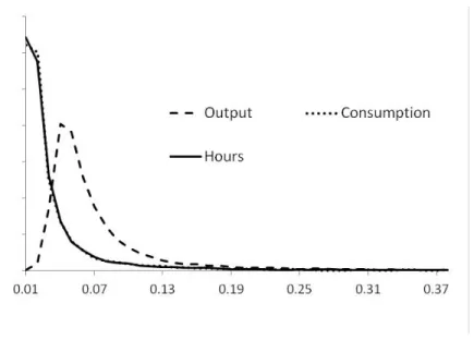
Figure 1 presents the posterior distribution averaged over all models, of the pro-portion of the variance of ct; ht and yt over the business cycle due to investment
pro-portion due to neutral technology shocks constructed by averaging over all models. These estimates are obtained from 30,000 draws from the posterior of each model. The plots show an amount of mass at zero for all three variables suggesting a slightly larger role for non-technology shocks. Relatively, the investment speci…c technology shocks are far more important than the neutral technology shocks and the propor-tions have considerable mass away from zero. The proportion of variation due to neutral technology shocks has little mass above 15%. We computed the same poste-rior densities as those reported in Figures 1 and 2 but using the CC, KPSW and the best models, as well as for all models in which the Great Ratios are the cointegrating relations. These estimates all share similar forms and pairwise comparisons showed no stochastic dominance of any distribution over any other.
Table 4 reports estimates of the mean proportions of the variance over the business cycle due to zI;t and zN;t for a range of models and model sets. The single models
considered are those used by CC, KPSW and the best model in our model set. The model sets we consider are, …rst, the set of all models and, second, the set of all models in which the Great Ratios are stable. Comparing across di¤erent models and model sets, the proportions appear relatively robust to speci…cation. The CC model is the only one that does not include the Great Ratios as stable cointegrating relations and we see that this results in slightly higher proportions of the variance due to investment speci…c technology shocks for output and consumption, although
the di¤erence is not large. Imposing the Great Ratios (as in KPSW, the best model and the set of all models with stable Great Ratios) slightly reduced the role ofzI;tin
business cycle variation for consumption and output, but not for investment. Overall, the technology shocks explain between 26% and 38% of the variation over the business cycle for these variables.
Relatively speaking, the investment speci…c technology shocks seem far more im-portant than the neutral technology shocks as they explain between 70% and 97% of the total variation due to technology shocks.
Table 4 reports the 95% credible intervals for the variance decompositions for the models and model sets we consider.12 An interesting point that arises from a
study of these intervals is that allowing for model uncertainty does not necessarily increase the degree of uncertainty about the variance decompositions. The last two columns of this table report results for sets of models: all models; and all models with balanced growth restrictions. In many cases the credible intervals in these columns are narrower than those for the single model estimates in the …rst three columns. We attribute this e¤ect, through correlations among outputs, to something analogous to the well know variance reduction from diversi…cation in an investment portfolio of …nancial assets.
12We are grateful to Frank Schorfheide for suggesting the inclusion of these intervals and to
inves-tigate the implications of model uncertainty and parameter uncertainty in the posterior distributions of the variance decompositions.
Propagation of Shocks: We conclude by discussing the responses in investment price, hours, output, consumption and investment to both investment speci…c and neutral technology shocks. The percentiles of the posterior distribution of these responses are shown in the panels in Figure 3. The left panels show responses to an investment speci…c shock, zI;t, while the right panels show responses to a neutral
technology shock, zN;t. Included in each panel is the mean impulse responses to the
technology shocks constructed from 30,000 draws of the parameters in each included model. It is immediately apparent that most of the densities have mass near zero. Note that these plots incorporate much more uncertainty than the usual ones that condition upon a model and so cannot be interpreted in the same way. The densities in Figure 3 re‡ect both parameter and model uncertainty and so any intervals will naturally be much wider and so can lead to di¤erent conclusions. Unlike with the variance decompositions, we do not bene…t from model averaging in estimation of impulse responses.
The mean path of investment price pt to shocks inzI;t and zN;t are very much as
would be expected from the model of Fisher and agree with the form of his simulated and estimated responses. The plot of the posterior response of pt to an investment
speci…c shock is persistently negative, while the response to a neutral technology shock shows only a slightly positive response, again agreeing with the results of Fisher. Output has a positive response to both shocks and the sizes of the responses are
similar in magnitude to those of Fisher, with a stronger and more persistent response tozN;t. Neither consumption nor investment display the persistent or large responses
suggested by Fisher’s simulations. In contrast to the simulations of Fisher, investment has an initially negative, then positive then declining response to investment speci…c technology shocks. Investment simply declines in response to neutral technology shocks. The response of hours worked di¤ers depending upon the type of technology shock in that investment speci…c shocks lead to an eventual fall in hours worked while the neutral shocks have a positive and persistent e¤ect. The magnitudes of the responses in hours is slightly smaller than those of Fisher. Both our results and those of Fisher suggest persistence in the response, however, our responses to investment speci…c shocks di¤er from those reported in Fisher (2006) in an important respect. Our results show a fall in hours worked while Fisher’s results suggest an increase in hours worked.
While many of the mean paths agree with those of Fisher (2006), the extra un-certainty leads to an important di¤erence in the conclusions. With the exception of the response of investment price to zI;t; the mean paths are not far from zero if we
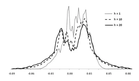
take the full posterior as the metric for distance. The posterior credible intervals for many of the responses encompass the origin but these intervals do not capture all of the information on the densities. The densities for the responses of the investment price to a neutral technology shock in Figure 4 at three horizons give an impression
of the general form and evolution of the response densities for other variables. The leptokurtic form and mass generally around zero is representative of the responses of at; yt; ht; ct and xt to investment speci…c shocks, and of ht to neutral technology
shocks.
The responses ofat;yt; ctandxtto neutral technology shocks show a very di¤erent
response. As an example, Figure 5 presents the posterior distribution of the response of outputytto an neutral technology shock at three di¤erent horizons. These densities
all have platykurtic forms for responses after one or two periods. However, they become increasingly bimodal at the time since the shock increases. This bimodality is not due to di¤erent models producing di¤erent paths as the responses for the best model in Table 1 produced very similar responses. A number of possible explanations exist, and one is that the identifying restrictions, at least for zN;t, disagree with the
data. However, as we are using just identifying restrictions it is not possible for us to report evidence at this point on this question.
Table 4: Estimated proportion of variance over the business cycle due to the investment-speci…c technology shock, zI;t, and the neutral technology
shocks, zN;t. 95% Credible intervals are shown in parentheses.
CC KPSW Best All Balanced
model model model models Growth models Consumption - ct zI;t 0.299 0.179 0.212 0.223 0.212 (0.02,0.75) (0.01,0.53) (0.02,0.55) (0.02,0.58) (0.02,0.55) zN;t 0.050 0.018 0.041 0.038 0.040 (0.00,0.20) (0.00,0.04) (0.00,0.15) (0.00,0.13) (0.00,0.14) Investment - xt zI;t 0.254 0.320 0.233 0.227 0.234 (0.02,0.62) (0.01,0.79) (0.02,0.60) (0.02,0.59) (0.02,0.60) zN;t 0.051 0.01 0.035 0.033 0.035 (0.00,0.20) (0.00,0.01) (0.00,0.13) (0.00,0.12) (0.00,0.13) Output - yt zI;t 0.281 0.160 0.202 0.216 0.202 (0.02,0.69) (0.01,0.44) (0.02,0.53) (0.02,0.56) (0.02,0.53) zN;t 0.097 0.045 0.082 0.076 0.081 (0.02,0.29) (0.02,0.08) (0.02,0.22) (0.02,0.20) (0.02,0.22)
Figure 1: Posterior densities of the proportion of the variance over the business cycle of output, consumption and hours that is due to investment speci…c technology shocks, zI;t.
6 Conclusions.
This paper presents a Bayesian model averaging approach in order to investigate the empirical support for several features of the DSGE type of real business cycle model of Fisher (2006) which we subject to two types of technology shocks. An important component of this model is the restrictions of long run responses that are used to identify investment speci…c and neutral technology shocks. For many of the features implied by this model we …nd reasonable support and some, such as stability of the Great Ratios, receive quite strong support, although not before 1984. Further, the
Figure 2: Posterior densities of the proportion of the variance over the business cycle of output, consumption and hours that is due to neutral technology shocks, zN;t.
impulse responses demonstrate that the predictions of the model are quite plausible although there is considerable uncertainty around these estimates.
The methodology is an important contribution of this paper. The approach re-sults in unconditional inference on these features of the vector autoregressive model as the e¤ect of any one model on the inference has been averaged out, and so model uncertainty is incorporated into the analysis. Techniques are developed for estimat-ing marginal likelihoods for models de…ned by such features as the number of stable relations (cointegration rank), overidentifying equilibrium restrictions, deterministic processes and short-run dynamics. To account for structural breaks and model switch-ing, methods are presented to make inference computationally feasible in a very large
set of multidimensional models.
The methods presented in this paper, without the structural breaks, have already found applications in several other areas. Koop, Potter and Strachan (2005) inves-tigate the support for the hypothesis that variability in US wealth is largely due to transitory shocks. They demonstrate the sensitivity of this conclusion to model un-certainty. Koop, León-González and Strachan (2008) develop methods of Bayesian inference in a ‡exible form of cointegrating VECM panel data model. These methods are applied to a monetary model of the exchange rate commonly employed in inter-national …nance. Other current work includes investigating the impact of oil prices on the probability of encountering the liquidity trap in the UK and stability of the money demand relation for Australia.
We end with mentioning two topics for further research. First, although our mix-ing over priors partially addresses this issue, there remains the issue of the robustness of the results with respect to wider prior and model speci…cations. Very natural extensions of the approach in this paper are to consider forms of time variation in the model itself as Cogley and Sargent (2001, 2005) and Primiceri (2005) do for the VAR. These papers suggest there is considerable variation in the parameters, partic-ularly over the 1970s. However, the reduced rank restrictions due to cointegration introduce further conceptual and computational issues for time varying models and a …rst example of how to implement such a time varying VECM is presented in Koop,
León-González and Strachan (2011). Alternatively, in using a SVAR for business cy-cle analysis one may use prior information on the length and amplitude of the period of oscillation (see Harvey, Trimbur and van Dijk 2007). Unresolved issues in this work include systematic use of inequality conditions which imply a more intense, or better, use of MCMC algorithms. Extending this approach to large model sets is yet to be considered and, given the computational issues, remains a challenge. Second, one may use the results of our approach in explicit decision problems in international and …nancial markets like hedging currency risk or evaluation of option prices.
Author A¢ liations: Rodney W. Strachan (Corresponding author), Research School of Economics, The Australian National University. Strachan is also a Fellow of The Centre for Applied Macroeconomic Analysis. Herman K. van Dijk Econo-metric Institute, Erasmus University Rotterdam and EconoEcono-metrics Department VU University Amsterdam. Van Dijk is an Honorary Fellow of the Tinbergen Institute. Both authors are Senior Fellows of the Rimini Centre for Economic Analysis.
7 Appendix
Identi…cation of the technology shocks: In this appendix we detail how the two technology shocks are identi…ed by the zero restrictions onC 1=2 shown in Section 3.
Let e1=2 denote any unique decomposition of such that = e1=2e1=20. This could be the unique Cholesky decomposition into a lower triangular matrix or taken from
the square root of the singular value decomposition. As we use the singular value decomposition below we will give this de…nition for e1=2. Take the singular value decomposition of then nmatrixAasA=U SV0 whereU 2O(n),V 2O(n)where
O(n) is the orthogonal group of n n matrices, and S =diag(s1; s2; : : : ; sn) where
si 0: A square root ofA may be obtained by the construction A1=2 =U S1=2V0:
To identify zt we need to choose an orthogonal matrix Ue such that 1=2 = e1=2Ue
such that = 1=2 1=20 = e1=2UeUe0e1=20 = e1=2e1=20.
Let c1 be (1 n) vector of the …rst row ofCe1=2 and let c2 be the (1 n 1) of the second to last elements in the second row ofCe1=2:Next let the projection matrix
projecting into the space of c1 be P1 = c10(c1c10) 1c1: Similarly, let the projection
matrix projecting into the space of c2 beP2:
ThenUe =U1U2 whereU1 is the orthogonal matrix spanning the column space of
the singular value decomposition of P1 =U1SV0: Further,
U2 = 2 6 6 4 1 0 0 U22 3 7 7 5
where U22 is the orthogonal matrix spanning the column space of the singular value
decomposition of P2 =U22SV0: We can then de…ne z
8 References.
Bates, J. M., and C. W. J. Granger, “The Combination of Forecasts,”Operational Research Quarterly 20 (1969), 451–468.
Centoni, M. and G. Cubbada, “Measuring the business cycle e¤ects of permanent and transitory shocks in cointegrated time series,”Economics Letters 80 (2003), 45-51. Chang, Y., and F. Schorfheide, “Labor-Supply Shifts and Economic Fluctuations,”
Journal of Monetary Economics 50(8) (2003), 1751-1768.
Chang, Y., Doh, T., and F. Schorfheide, “Non-stationary Hours in a DSGE Model,”
Journal of Money, Credit, and Banking, 39(6) (2007), 1357-1373.
Cogley, T., and T. J. Sargent, “Evolving Post-World War II US In‡ation Dynamics,”
NBER Macroeconomics Annual 16 (2001), 331–373.
Cogley, T., and T. J. Sargent, “Drifts and Volatilities: Monetary Policies and Out-comes in the Post WWII U.S.,”Review of Economic Dynamics 8 (2005), 262-302. Del Negro, M., and F. Schorfheide, “Bayesian Macroeconometrics”in: J. Geweke, G. Koop, and H.K. van Dijk, ed., Handbook of Bayesian Econometrics (2011), Chapter 7, pp. 293-389.
Diebold, F.X. and J. Lopez, “Forecast Evaluation and Combination,”in G.S. Maddala and C.R. Rao (eds.),Handbook of Statistics (Amsterdam: North-Holland 1996), 241-268.
Draper, D., “Assessment and propagation of model uncertainty (with discussion),”
Journal of the Royal Statistical Society Series B 56 (1995), 45-98.
Fernández, C., E. Ley, and M. Steel, “Model uncertainty in cross-country growth regressions,”Journal of Applied Econometrics 16 (2001), 563-576.
Fisher, J. D. M. “The Dynamic E¤ects of Neutral and Investment-Speci…c Technology Shocks,” Manuscript, Fed. Reserve Bank Chicago 2005.
Fisher, Jonas D. M. “The Dynamic E¤ects of Neutral and Investment-Speci…c Tech-nology Shocks,”Journal of Political Economy 114 (2006), 413-451.
Geweke, J. “Bayesian reduced rank regression in econometrics,”Journal of Econo-metrics 75 (1996), 121-146.
Geweke J. Contemporary Bayesian Econometrics and Statistics (Wiley: Hoboken, NJ, 2005).
Geweke, J., and G. Amisano, “Hierarchical Markov Normal Mixture Models with Ap-plications to Financial Asset Returns,”Journal of Applied Econometrics 26 (2011), 1-29.
Greenwood, J., Z. Hercowitz, and P. Krusell, “Long-Run Implications of Investment-Speci…c Technological Change,”The American Economic Review 87 (1997), 342-62.
Harvey, A.C., T.M. Trimbur and H. K. van Dijk, “Trends and cycles in economic time series: A Bayesian approach,”Journal of Econometrics 140 (2007), 618-649.
Hendry, D. F. & M. P. Clements, “Pooling of Forecasts,”Econometrics Journal 5
(2002), 1-26.
Hodges, J., “Uncertainty, policy analysis and statistics,”Statistical Science 2(1987), 259-291.
Hoogerheide, L.F., R. Kleijn, F. Ravazzolo, H.K. Van Dijk, and M. Verbeek, “Forecast Accuracy and Economic Gains from Bayesian Model Averaging using Time Varying Weights,”Journal of Forecasting 29 (2010), 251-269.
Johansen, S.,Likelihood-based Inference in Cointegrated Vector Autoregressive Models
(New York: Oxford University Press, 1995).
King, R., C.I. Plosser, and S. Rebelo, “Production, growth, and business cycles I: The basic neoclassical model,”Journal of Monetary Economics 21 (1988), 195-232. King, R.G., C.I. Plosser, J.H. Stock, and M.W. Watson, “Stochastic trends and economic ‡uctuations.”The American Economic Review 81 (1991), 819-840.
Koop, G.,Bayesian Econometrics (Wiley, Chichester, 2003).
Koop, G., R. León-González and R. W. Strachan, “Bayesian inference in a cointe-grating panel data model”Advances in Econometrics, Volume 23 (2008).
Koop, G., R. León-González and R. W. Strachan, “E¢ cient posterior simulation for cointegrated models with priors on the cointegration space”Econometric Reviews 29
Koop G., R. León-González and R. W. Strachan, “Bayesian Inference in the Time Varying Cointegration Model,”The Journal of Econometrics 165 (2011), 210-220. Koop G., R. León-González and R.W. Strachan, “A Reversible Jump algorithm for inference using instrumental variables” forthcoming in The Journal of Econometrics
(2012).
Koop, G. and S. Potter, “Bayesian Analysis of Endogenous Delay Threshold Models,”
Journal of Business and Economic Statistics 21 (2003), 93-103.
Koop, G., S. Potter and R.W. Strachan, “Re-examining the Consumption-Wealth Relationship: The Role of Model Uncertainty,”Journal of Money, Credit and Banking 40 (2005), No. 2–3, 341-367.
Kydland, F. and E. Prescott, “Time to build and aggregate ‡uctuations,” Economet-rica 50 (1982), 173-208.
Leamer, E., Speci…cation Searches (New York: Wiley, 1978).
Litterman, R. B., “A Bayesian procedure for forecasting with vector autoregressions,” Massachusetts Institute of Technology, Mimeo (1980).
Litterman, R. B., “Forecasting with Bayesian vector autoregressions — Five years of experience,”Journal of Business and Economic Statistics 4 (1986), 25–38.
McConnell, M. and G. Perez-Quiros, “Output Fluctuations in the United-States: What Has Changed Since the Early 1980’s,”American Economic Review 90 (2000),
1464–1476.
Min, C. and A. Zellner, “Bayesian and non-Bayesian methods for combining models and forecasts with applications to forecasting international growth rates,”Journal of Econometrics 56 (1993), 89-118.
Newbold, P. & D. Harvey, “Tests for Multiple Forecast Encompassing,”Journal of Applied Econometrics 15 (2001), 471–482.
Ni, S. X. and D. Sun, “Noninformative Priors and Frequentist Risks of Bayesian Estimators of Vector-Autoregressive Models,”Journal of Econometrics 115 (2003), 159-197.
Poirier, D.,Intermediate Statistics and Econometrics: A Comparative Approach (Cam-bridge: The MIT Press, 1995).
Primiceri, G., “Time Varying Structural Vector Autoregressions and Monetary Pol-icy,”Review of Economic Studies 72 (2005), 821-852.
Raftery, A. E., D. Madigan, and J. Hoeting “Bayesian model averaging for linear regression models,”Journal of the American Statistical Association 92 (1997), 179– 191.
Sala-i-Martin, X., G. Doppelho¤er, and R. Miller, “Determinants of long-term growth: A Bayesian averaging of classical estimates (BACE) approach,”American Economic Review 94 (2004), 813-835.
Stock, J. H. and M. W. Watson, “Has the Business Cycle Changed and Why?,”
NBER Macroeconomics Annual, Volume 17 (MIT Press, 2002).
Strachan, R. W. and B. Inder, “Bayesian Analysis of The Error Correction Model,”
Journal of Econometrics 123 (2004), 307-325.
Strachan, R. W. and H. K. van Dijk, “Evidence on a DSGE Business Cycle Model subject to Neutral and Investment-Speci…c Technology Shocks using Bayesian Model Averaging,”CAMA Working Paper 3/2012 (2012).
Tanner, M. A.,Tools for statistical inference : methods for the exploration of posterior distributions and likelihood functions. (2nd Edition). (Springer Series in Statistics, New York: Springer, 1993).
Terui, N. and H. K. van Dijk, “Combined forecasts from linear and nonlinear time series models,”International Journal of Forecasting 18(3) (2002), 421-438.
Villani, M., “Bayesian prediction with cointegrated vector autoregressions,” Interna-tional Journal of Forecasting 17 (2001), 585-605.
Wright, Jonathon H., “Bayesian Model Averaging and exchange rate forecasts,” Jour-nal of Econometrics 146 (2008), 329-341.
Figure 3: The 20%, 40%, 50%, 60% and 80% percentiles of the posterior distribution of the response of investment price, p, output, y, consumption, c, investment, x, and hours, h, to investment speci…c, I, and neutral, N, technology shocks. The x-axis is
Figure 4: Posterior densities of the impulse responses of investment price, pt; to a
neutral technology shock, zN;t, at horizons h = 1, h = 10 and h = 20. The x-axis is
Figure 5: Posterior densities of the impulse responses of output to a neutral technol-ogy shock, zN;t, at horizons h = 1, h = 10 and h = 20. The x-axis is in percent.