Instructions for use
Title Bayesian Dynamic Panel-Ordered Probit Model and Its Application to Subjective Well-Being
Author(s) Hasegawa, Hikaru
Citation Communications in Statistics : Simulation and Computation, 38(6), 1321-1347https://doi.org/10.1080/03610910902903133
Issue Date 2009-06
Doc URL http://hdl.handle.net/2115/43089
Rights This is an electronic version of an article published in Communications in Statistics : Simulation and Computation,38(6) June 2009, 1321-1347. Communications in Statistics : Simulation and Computation is available online at: http://www.informaworld.com/openurl?genre=article&issn=0361-0918&volume=38&issue=6&spage=1321
Type article (author version)
Bayesian Dynamic Panel Ordered Probit Model
and Its Application to Subjective Well-Being
Hikaru Hasegawa
∗Graduate School of Economics and Business Administration Hokkaido University
Abstract
This article proposes a Bayesian method for estimating the dynamic panel ordered probit model. We compare four alternative algorithms for the estimation of ordered probit models. Furthermore, this article presents the empirical results of the application of the dynamic ordered probit model to subjective well-being based on the micro-level survey data extracted from the Japanese Panel Survey of Consumers. The results of the application reveal that income and savings have positive effects on life satisfaction, whereas our posterior results show that marriage and labor force partici-pation have negative effects on the same.
Keywords Generalized Gibbs sampler; Life satisfaction; Markov chain Monte Carlo (MCMC); Well-being function.
Mathematics Subject Classification 62F15; 62P20.
Proposed running head Bayesian Dynamic Panel Ordered Probit Model.
∗Address correspondence to Hikaru Hasegawa, Graduate School of Economics and Business
Administration, Hokkaido University, Kita 9, Nishi 7, Kita-ku, Sapporo 060-0809, Japan; E-mail: [email protected].
1
Introduction
In a questionnaire survey concerning subjective outcomes such as life satisfac-tion, choices are often ordinally arranged. An ordered probit model can be used to statistically analyze the data on such ordinal choices. From the frequentist viewpoint, the ordered probit model can be estimated by using the maximum likelihood (ML) method.1
On the other hand, posterior distributions play a central role in the Bayesian analysis. Recent developments in the Markov chain Monte Carlo (MCMC) method enable us to sample unobservable parameters from their posterior dis-tributions even if the models are complicated. Albert and Chib (1993) propose the Bayesian approach for the estimation of the ordered probit model by using the MCMC method. They use the latent variable representation for the estima-tion of ordered probit models. Cowles (1996) and Nandram and Chen (1996) propose sampling algorithms for the Bayesian ordered probit model that are more efficient than that of Albert and Chib (1993). Further, Jeliazkov et al. (2008) review the identification and modeling problems in the ordered probit models.
This article proposes a Bayesian dynamic panel ordered probit model. Al-though M¨uller and Czado (2005) consider the Bayesian estimation of the au-toregressive ordered probit model by adapting Liu and Sabatti’s (2000) method, they do not deal with the dynamic panel data model. Our model uses the latent variable representation for ordinal choices, and the model for latent variable is a dynamic version of the Hausman and Taylor (1981) model. The dynamic panel data models with unobserved effects encounter a problem with respect to the initial conditions (Hsiao, 2003, Section 7.5). Wooldridge (2005) proposes a gen-eral method for resolving this problem in dynamic panel models including the ordered probit model in the non-Bayesian framework. One of the contributions of this article is to provide the Bayesian estimation framework that formulates the initial conditions problem in dynamic panel models. According to Jeliazkov et al. (2008), there are several kind of estimation algorithms for ordered pro-bit models. Using the simulated data and the real data, this article compares the performances of estimation algorithms within the framework of Bayesian dynamic panel ordered probit model.
We apply the Bayesian dynamic panel ordered probit model to subjective well-being as a real data application.2 The number of studies on well-being continue to increase and form a large amount of the literature.3 One of the important issues in well-being studies is the choice of the sources of well-being, that is, selecting the explanatory variable of the well-being function (Frey and Stutzer, 2005, pp.213–217). As we will describe in Section 5, based on the ap-plication of the dynamic ordered probit model to the data on young Japanese women, income and savings are shown to have positive effects on well-being, whereas marriage and labor force participation are shown to have negative ef-fects.
The article proceeds as follows. In Section 2, we provide the Bayesian dy-namic panel ordered probit model. Section 3 describes the alternative four
1See, for example, Greene (2003, Chapter 21).
2In this article, we use life satisfaction as the measurement of well-being.
3See, for example, Blanchflower and Oswald (2004), Clark and Oswald (2002), and Frey and Stutzer (2002a,b, 2005).
algorithms for the estimation of the Bayesian dynamic panel ordered probit model. The comparisons among the four algorithms are provided in Section 4. Section 5 presents the empirical results of the application of the dynamic panel ordered probit model to subjective well-being, based on the micro-level survey data extracted from the Japanese Panel Survey of Consumers (JPSC), which is conducted by the Institute for Research on Household Economics. In Section 6, we provide a brief conclusion.
2
The Dynamic Panel Ordered Probit Model
In this section, we describe the Bayesian dynamic panel ordered probit model. Let yit denote the ordinal discrete response of individual i at time t for t =
0,1,· · · , T and i = 1,· · · , n; that is, yit = c for c = 1,· · ·, C, where t = 0
denotes an initial period. Further, letzitdenote the latent variable of individual
iat time tsuch that
yit=c if zit∈(γc−1, γc], t= 0,1,· · ·, T, i= 1,· · ·, n, c= 1,· · ·, C,
(1) whereγc is a cutoff point of ordinal response. We specify that
−∞=γ0< γ1= 0< γ2<· · ·< γC−1< γC=∞,
where the condition γ1 = 0 is required to establish the identifiability of the cutoff parameters.4 The latent variablez
it is assumed to be determined by the
following linear model: fori= 1,· · · , n, {
zit=ϕzi(t−1)+x′itβ+w′iδ+αi+uit, t= 1,· · ·, T
zi0=x′i0β0+wi′δ0+αi+ui0, t= 0,
where xit = (xit1,· · · , xitk)′ is a vector of time-variant explanatory variables,
wi = (wi1,· · · , wip)′ is a vector of cross-sectional time-invariant explanatory
variables, αi is a random effect, β = (β1,· · ·, βk)′, δ = (δ1,· · ·, δp)′, β0 = (β01,· · ·, β0k)′, andδ0= (δ01,· · ·, δ0p)′.5 We assume that uit are independent
and identically normally distributed with zero mean and unit variance, that is,
uit∼N(0,1). Then, we have
{
zit| · · · ∼N(ϕzi(t−1)+x′itβ+w′iδ+αi,1), t= 1,· · · , T
zi0| · · · ∼N(x′i0β0+w′iδ0+αi,1), t= 0
(2)
for i = 1,· · ·, n, where “| · · ·” denotes conditioning on the other unspecified variables in the equation.
To complete the Bayesian model, we introduce the prior distributions of the parameters (ϕ,β,δ,β0,δ0,α, γ), whereα= (α1,· · · , αn)′andγ= (γ2,· · ·, γC−1)′.
We assume that the prior distribution of the vector of random effectsα has a hierarchical structure.6 The prior distributions are specified as follows:
p(ϕ,β,δ,β0,δ0,α, µ, τ,γ)
=p(ϕ)p(β)p(δ)p(β0)p(δ0)p(α|µ, τ)p(µ)p(τ)p(γ). (3) 4See, for example, Albert and Chib (1993, p.673) and Johnson and Albert (1999, p.131). 5This model is a dynamic version of the Hausman and Taylor (1981) model. See, for example, Baltagi (2001, p.139).
Further, from Bayes’ theorem, the joint posterior distribution can be written as follows: p(ϕ,β,δ,β0,δ0,α, µ, τ,γ,z,z0|y,y0)∝p(ϕ,β,δ,β0,δ0,α, µ, τ,γ,z,z0) ×p(y,y0|ϕ,β,δ,β0,δ0,α, µ, τ,γ,z,z0) =p(ϕ,β,δ,β0,δ0,α, µ, τ,γ) × n ∏ i=1 [{ p(zi|ϕ,β,δ, αi, µ, τ,γ, zi0)p(yi|ϕ,β,δ, αi, µ, τ,γ,zi, zi0) } ×{p(zi0|ϕ,β0,δ0, αi, µ, τ,γ)p(yi0|ϕ,β0,δ0, αi, µ, τ,γ, zi0) }] , (4) where yi= (yi1, yi2,· · · , yiT)′, zi= (zi1, zi2,· · ·, ziT)′, i= 1,· · · , n y= (y′1,y2′,· · · ,y′n)′, z= (z′1,z2′,· · ·,z′n)′ y0= (y10, y20,· · ·, yn0)′, z0= (z10, z20,· · ·, zn0)′.
3
Algorithms for the Estimation of the Bayesian
Dynamic Panel Ordered Probit Model
Jeliazkov et al. (2008) consider three algorithms for the univariate ordered probit model, that is to say, the algorithms based on Albert and Chib (1993), Albert and Chib (2001) and Chen and Dey (2000). It is known that the MCMC sample for the cutoff points by using the algorithm of Albert and Chib (1993) has high autocorrelation. To take care of this problem, Albert and Chib (2001) and Chen and Dey (2000) propose the algorithms for drawing the cutoff points by transforming them. Furthermore, M¨uller and Czado (2005) consider the Bayesian estimation of the autoregressive ordered probit model by adapting Liu and Sabatti’s (2000) method. In this section, we extend these existing algorithms to the Bayesian dynamic ordered probit model.
3.1
Algorithm based on Albert and Chib (1993)
The prior distributions are specified as follows: ϕ∼N( ˜ϕ,ω˜)1(ϕ∈(−1,1)), β∼N( ˜β,B˜), δ∼N(˜δ,D˜) β0∼N( ˜β0,B˜0), δ0∼N(˜δ0,D˜0) αi ∼N(µ, τ), i= 1,· · ·, n, µ∼N(˜µ,κ˜), τ−1∼Gam(˜a,˜b) p(γ)∝1(γ∈C), C={γ: 0< γ2<· · ·< γC−1<∞}, (5)
where 1(·)is an indicator function and Gam(a, b) denotes a gamma distribution with parametersa, b. The algorithm of drawing the parameters in the dynamic panel ordered probit model based on the algorithm of Albert and Chib (1993) is as follows:7
Algorithm 1:
1. Sampleϕ,β,δ,β0,δ0,α, µ, τfrom their full conditional distributions (FCDs).
2. Sample z,z0 from their FCDs. 3. Sample γfrom its FCD.
3.2
Algorithm using Liu and Sabatti’s method (2000)
We can use the algorithm proposed in Liu and Sabatti (2000) for estimating our Bayesian dynamic ordered probit model. To apply Liu and Sabatti’s (2000) method, we specify the hyperparameters in the prior distributions (5) as follows:
˜
β=0, δ˜=0, β˜0=0, ˜δ0=0, µ˜= 0.
The algorithm of drawing the parameters in the dynamic panel ordered probit model as per the algorithm of Liu and Sabatti (2000) is as follows:8
Algorithm 2:
1. Sample ϕ,β,δ,β0,δ0,α, µ, τ from their FCDs. 2. Sample z,z0 from their FCDs.
3. Sample γfrom its FCD.
4. Implement Liu and Sabatti’s generalized Gibbs sampler.
3.3
Algorithm based on Albert and Chib (2001)
Albert and Chib (2001) propose the algorithm for drawing the cutoff points by transforming them as follows:
ζc= log(γc−γc−1), c= 2,· · · , C−1, (6)
where ζ(γ) = (ζ2,· · ·, ζC−1)′ is unrestricted. Thus, we specify the prior
distri-bution of γ, p(γ) = p(ζ(γ)), as ζ(γ) ∼N( ˜ζ,G˜) based on the transformation (6). The algorithm of drawing the parameters in the dynamic panel ordered probit model based on the algorithm of Albert and Chib (2001) is as follows:9
Algorithm 3:
1. Sample ϕ,β,δ,β0,δ0,α, µ, τ from their FCDs. 2. Sample z,z0 from their FCDs.
3. Sample ζfrom the Metropolis-Hastings (M-H) algorithm.
4. Calculateγc= c
∑
j=1
expζj, c= 2,· · · , C−1.
8The details of this sampling algorithm are provided in Appendix B. Further, to use the scale group defined in Appendix B, we have to specify the hyperparameters in the prior distributions ˜β=0, ˜δ=0, ˜β0=0, ˜δ0=0and ˜µ= 0.
3.4
Algorithm based on Chen and Dey (2000)
Although the unit variance of disturbance, that is, var(uit) = 1, is standard
identification restriction, there are another ways to identify the ordered probit model. Nandram and Chen (1996) and Chen and Dey (2000) provide an iden-tification restriction based on the reparameterization of the cutoff points, that is,γC−1= 1. Under this identification condition, model (2) can be modified as
{
zit| · · · ∼N(ϕzi(t−1)+x′itβ+w′iδ+αi, σ2), t= 1,· · ·, T
zi0| · · · ∼N(x′i0β0+w′iδ0+αi, σ2), t= 0
(7)
fori= 1,· · · , n. Further, Chen and Dey (2000) propose the following transfor-mation of cutoff points:
ζc= log ( γc−γc−1 1−γc ) , c= 2,· · · , C−2, (8)
whereζ(γ) = (ζ2,· · ·, ζC−2)′ is unrestricted. The prior distributions are
speci-fied as follows:
p(ϕ,β,δ,β0,δ0,α, µ, τ, σ2,γ)
=p(ϕ)p(β)p(δ)p(β0)p(δ0)p(α|µ, τ)p(µ)p(τ)p(σ2)p(γ). (9) We specify the same prior distributions of parameters as in (5) except for σ2 andγ. Their prior distributions are specified as follows:
σ−2∼Gam(˜c,d˜), ζ(γ)∼N( ˜ζ,G˜), (10) where the prior distribution ofγ,p(γ) =p(ζ(γ)), is based on the transformation (8). The algorithm of drawing the parameters in the dynamic panel ordered probit model based on the algorithm of Nandram and Chen (1996) and Chen and Dey (2000) is as follows:10
Algorithm 4:
1. Sample ϕ,β,δ,β0,δ0,α, µ, τ, σ2from their FCDs. 2. Sample z,z0 from their FCDs.
3. Sample ζfrom the M-H algorithm. 4. Calculateγc=
γc−1+ expζc
1 + expζc
, c= 2,· · · , C−2.
4
Numerical Example with Simulated Data
This section provides a numerical example with simulated data for comparing the performances of four algorithms. In the numerical example, we set n = 200 and T = 9, and the ordered response variables yit (i = 1,· · · ,200, t =
0,1,· · · ,9) are assumed to take four values, that is, yit = 1,2,3,4. We also
assume that the latent variables are distributed as follows: {
zit| · · · ∼N(ϕzi(t−1)+xitβ1+wiδ1+αi,1), t= 1,· · ·,9
zi0| · · · ∼N(xi0β01+wiδ01+αi,1), t= 0
fori= 1,· · · ,200, where the parameters and the variables are specified as:
ϕ= 0.5, β1=β01= 2.0, δ1=δ01= 1.5, γ2= 5.0, γ3= 10.0
xi0∼N(1,3), xit= 0.3xi(t−1)+vit, vit∼N(0,1)
wi∼N(2,4), αi∼N(−3,4).
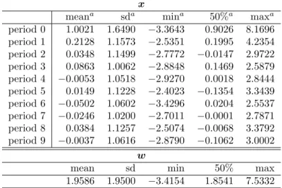
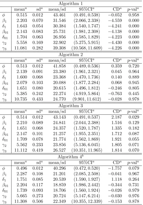
The summary statistics of these variables are provided in Tables 1 and 2. The MCMC simulation was run for 12,000 iterations with the thinning in-terval equal to 5; the first 2,000 samples were discarded as the burn-in period.11 The posterior results obtained thereafter are generated using Ox version 5.00 (Doornik, 2007). Table 3 presents the posterior results for the estimation of ϕ,
β1, δ1, β01, δ01, and γ.12 In Table 3, “95%CI” denotes the 95% credible in-terval. “CD” denotes the convergence diagnostic statistic proposed by Geweke (1992).13 The sixth column of Table 3 shows thep-values for CD.
According to CD, Algorithm 1 does not exhibit good performances. ϕ in Algorithm 3 does not converge. By contrast, Algorithms 2 and 4 perform well according to CD. In the next section, we use Algorithms 2 and 4 for estimating the dynamic ordered probit model by using the real data.
5
Application to the Analysis of Life
Satisfac-tion
5.1
Data
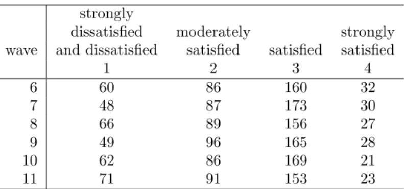
Our empirical analysis uses the micro-level survey data extracted from the Japanese Panel Survey of Consumers (JPSC), which is conducted by the In-stitute for Research on Household Economics. Since 1993, the survey has been administered to 1,500 women representative of the entire female population in the age range of 24–34 years in 1993. The JPSC data provide several measures of satisfaction pertaining to young women in Japan. This article employs the 6th wave (1998) to the 11th wave (2003) of JPSC data. From the above panel data, we select the data pertaining to women who responded to the question on life satisfaction over a period of 6 years from 1998 through 2003. Finally, the total number of recorded responses stood at 338.
We use the following variables:
11We obtained 12,000 samples by running 60,000 iterations and sampling one observation at every five iterations. After obtaining 12,000 samples, we discarded the first 2,000 samples. 12The results of parameters in Algorithm 4 except forϕare those of the transformed pa-rameters divided byσ.
13CD can be defined as follows: for the given sequence {g(j) |j = 1,2,· · ·, n
s}, if the sequence is stationary, CD= g¯A−¯gB ˆ SA(0)/nA+ ˆSB(0)/nB →N(0,1), where ¯ gA= 1 nA nA ∑ j=1 g(j), g¯B= 1 nB ns ∑ j=n∗ g(j) (n∗=ns−nB+ 1),
and ˆSA(0) and ˆSB(0) denote consistent spectral density estimates. In this numerical example,
we setnA= 1,000 and nB = 5,000, and calculate ˆSA(0) and ˆSB(0) using Parzen windows
• ordinal dependent variables: lifesat(y,z)
• time-variant explanatory variables: married (x1), loginc (x2), logsav (x3),inwork(x4)
• cross-sectional time-invariant explanatory variables: age (w1) and educ
(w2),
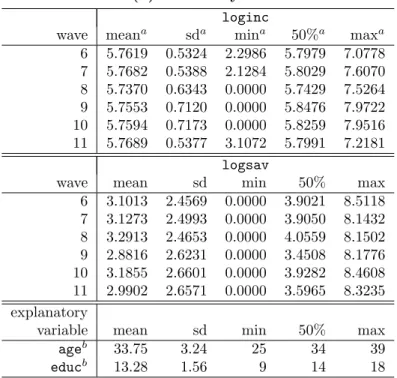
where lifesat denotes life satisfaction, for which the number of ordinal re-sponses isC= 4;14married(x1), a dummy variable that takes 1 if a respondent is married, and 0 otherwise; loginc (x2), the logarithm of the previous year’s per capita real annual household income (ten-thousand yen, base year = 2000);
logsav (x3), the logarithm of per capita real household savings (ten-thousand yen, base year = 2000); inwork (x4), a dummy variable that takes 1 if a re-spondent is working, and 0 otherwise.15 In addition,
age (w1) represents the age of the respondent in 1998; and educ (w2), the years of education of the respondent. The summary statistics of these variables are provided in Tables 4 and 5.
The estimated well-being functions are as follows:
zit=ϕzi(t−1)+β1xit1+β2xit2+β3xit3+β4xit4 +δ1wi1+δ2wi2+αi+uit, t= 1,· · ·,5
zi0=β01xi01+β2xi02+β3xi03+β4xi04+δ01wi1+δ02wi2+αi+ui0, where the initial period (t= 0) is year 1998.
5.2
Posterior results
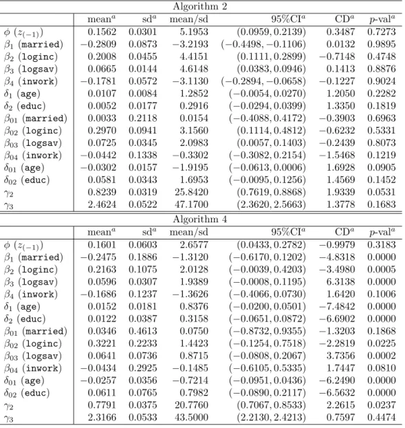
The MCMC simulation was run for 30,000 iterations with the thinning interval equal to 5; the first 10,000 samples were discarded as the burn-in period.16 Table 6 presents the posterior results for the estimation of ϕ, β, δ, β0, δ0, andγ.17 According to the convergence diagnostic statistic (CD), parameters in Algorithm 4 except forϕ,β4,β01,β04andγ3 do not converge. By contrast, all parameters in Algorithm 2 converge. Therefore, we use the posterior results in Algorithm 2. The following points can be observed from the posterior results in Algorithm 2.
• According to the 95% credible interval, the lagged latent variable (z(−1)) has a significantly positive effect on life satisfaction.18
14The number of ordinal categories of life satisfaction is originallyC= 5, including “strongly dissatisfied,” “dissatisfied,” “moderately satisfied,” “satisfied,” and “strongly satisfied.” How-ever, since the frequency of “strongly dissatisfied” is small, this article combines two categories “strongly dissatisfied” and “dissatisfied” into a single category, “strongly dissatisfied and dis-satisfied.”
15In the case of zero income or zero savings, we setloginc(x
2) orlogsav(x3) equal to 0. Further, we use the consumer price index as a deflator for constructing real variables.
16We obtained 30,000 samples by running 150,000 iterations and sampling one observation at every five iterations. After obtaining 30,000 samples, we discarded the first 10,000 samples. 17The results of parameters in Algorithm 4 except forϕare those of the transformed pa-rameters divided byσ.
18Here, the term “significant” is used if the 95% credible interval for a parameter does not include zero. See also Koop (2003, p.124).
• Two dummy variables, the marriage (married) and labor force participa-tion dummies (inwork), have significantly negative effects on life satisfac-tion fort≥1, but they are not significant at the initial periodt= 0. • Income (loginc) and savings (logsav) have significantly positive effects
on life satisfaction for all the periods.
• The time-invariant explanatory variables (ageand educ) are not signifi-cant for all the periods.
• Three cutoff points (γ2,γ3, and γ4) are significantly estimated.
As in Wooldridge (2002, pp.505–506), we are more interested in the response probabilities Pr(yit =c) than in the coefficient parameters themselves. Table
7 shows the posterior results for the partial effects of the explanatory variables on the response probabilities.19 The following points can be observed from the posterior results in Table 7.
• The convergence of the posterior distributions can be confirmed from the
p-values for CD.
• z(−1), married, loginc, logsav, and inwork have significantly partial effects on the response probabilities, but the partial effects of age and
educon the response probabilities are not significant.
• The lagged latent variable (z(−1)) increases the probabilities Pr(y= 3) and Pr(y = 4) by 3.7 and 2.2 percent points, respectively; income (loginc) increases the probabilities Pr(y= 3) and Pr(y = 4) by 11.0 and 7.2 per-cent points, respectively; and savings (logsav) increases the probabilities Pr(y = 3) and Pr(y = 4) by 3.2 and 2.0 percent points, respectively. Therefore, income has the largest positive effect on life satisfaction in terms of the response probabilities.
• Per contra, the marriage dummy (married) decreases the probabilities Pr(y= 3) and Pr(y= 4) by 4.8 and 3.7 percent points, respectively. Fur-ther, the labor force participation dummy (inwork) decreases the proba-bilities Pr(y= 3) and Pr(y= 4) by 3.6 and 2.2 percent points, respectively. Therefore, marriage and labor force participation have negative effects on life satisfaction in terms of the response probabilities. The negative ef-fect of marriage on life satisfaction contrasts with the findings of previous studies.20 This may be attributable to the respondents of the sample. The respondents of the JPSC data are relatively young women, and most of the single women in the sample live with their parents. If young women do not live with their parents after marriage, the marriage would lead to a significant decline in single women’s standard of living, which would decrease their life satisfaction.
19The details of partial effects of the continuous explanatory variables are provided in Ap-pendix E.
6
Conclusion
This article proposed a Bayesian method for estimating the dynamic panel or-dered probit model, which addressed the initial conditions problem, and com-pared the four alternative algorithms for the model. Our result of simulated data suggested that the algorithms using Liu and Sabatti’s (2000) method and Chen and Dey (2000) perform well. In addition, this article provided the empir-ical results of the application of the dynamic ordered probit model to subjective well-being using the micro-level survey data obtained from the JPSC, which is conducted by the Institute for Research on Household Economics. The posterior results suggested that the algorithm using the Liu and Sabatti’s method exhibits a better performance than that of Chen and Dey (2000). Furthermore, as in Wooldridge (2002, pp.505–506), we focused on the response probabilities of the ordered probit model rather than on the coefficient parameters themselves. The posterior results revealed that income and savings have positive effects on life satisfaction in terms of the response probabilities, whereas our posterior results showed that marriage and labor force participation have negative effects.
A
Derivation of Algorithm 1
A.1
FCD of
ϕ
The full conditional distribution (FCD) ofϕis
ϕ| · · · ∼N( ˆϕ,ωˆ)1(ϕ∈(−1,1)), where ˆ ω= ( 1 ˜ ω + n ∑ i=1 T ∑ t=1 zi2(t−1) )−1 ˆ ϕ= ˆω [ ˜ ϕ ˜ ω + n ∑ i=1 T ∑ t=1 zi(t−1)(zit−x′itβ−w′iδ−αi) ] .
We can utilize Damien and Walker’s (2001) algorithm for sampling from a trun-cated normal distribution.21
21Using Damien and Walker’s algorithm, we can sampleϕfrom the following steps.
1. Letx=ϕ√−ϕˆ ˆ ω , we haveϕ∈(−1,1)⇔x∈ ( −1−ϕˆ √ ˆ ω , 1−ϕˆ √ ˆ ω ) . 2. Introduce the latent variableywhich has joint density withxgiven by
p(x, y)∝1(y∈(0,exp(−x2/2)))1(x∈(a,b)), wherea=−1√−ϕˆ ˆ ω , b= 1−ϕˆ √ ˆ ω . 3. We have the following FCDs:
y|x∼U ( 0,exp ( −x2 2 )) x|y∼U ( max { −1−ϕˆ √ ˆ ω ,− √ −2 logy } ,min { 1−ϕˆ √ ˆ ω , √ −2 logy }) .
A.2
FCD of
β
The FCD ofβ is β| · · · ∼N( ˆβ,Bˆ), where ˆ B= ( ˜ B−1+ n ∑ i=1 T ∑ t=1 xitx′it )−1 ˆ β= ˆB [ ˜ B−1β˜+ n ∑ i=1 T ∑ t=1 xit(zit−ϕzi(t−1)−w′iδ−αi) ] .A.3
FCD of
δ
The FCD ofδ is δ| · · · ∼N(ˆδ,Dˆ), where ˆ D= ( ˜ D−1+T n ∑ i=1 wiw′i )−1 ˆ δ= ˆD [ ˜ D−1δ˜+ n ∑ i=1 T ∑ t=1 wi(zit−ϕzi(t−1)−x′itβ−αi) ] .A.4
FCD of
β
0 The FCD ofβ0 is β0| · · · ∼N( ˆβ0,Bˆ0), where ˆ B0= ( ˜ B−01+ n ∑ i=1 xi0x′i0 )−1 ˆ β0= ˆB0 [ ˜ B−01β˜0+ n ∑ i=1 xi0(zi0−w′iδ0−αi) ] .A.5
FCD of
δ
0 The FCD ofδ0 is δ0| · · · ∼N(ˆδ0,Dˆ0), 4. Calculateϕ= ˆϕ+√ωx.ˆwhere ˆ D0= ( ˜ D−01+ n ∑ i=1 wiw′i )−1 ˆ δ0= ˆD0 [ ˜ D−01˜δ0+ n ∑ i=1 wi(zi0−x′i0β0−αi) ] .
A.6
FCD of
α
The FCD ofαi is αi| · · · ∼N( ˆαi,τˆ), i= 1,· · · , n, where ˆ τ= ( 1 τ +T+ 1 )−1 ˆ αi= ˆτ [ µ τ + T ∑ t=1 (zit−ϕzi(t−1)−x′itβ−wi′δ) + (zi0−xi′0β0−w′iδ0) ] .A.7
FCD of
µ
The FCD ofµis µ| · · · ∼N(ˆµ,κˆ), where ˆ κ= ( 1 ˜ κ+ n τ )−1 , µˆ= ˆκ ( ˜ µ ˜ κ+ 1 τ n ∑ i=1 αi ) .A.8
FCD of
τ
The FCD ofτ−1 is τ−1| · · · ∼Gam(ˆa,ˆb), where ˆ a= ˜a+n 2, ˆb= ˜b+1 2 n ∑ i=1 (αi−µ)2.A.9
FCD of
z
0 The FCD ofzi0is zi0| · · · ∼N ( ˆ zi0, 1 1 +ϕ2 ) 1(zi0∈(γc−1,γc]), i= 1,· · ·, n, where ˆ zi0= ϕ(zi1−x′i1β−w′iδ−αi) + (x′i0β0+w′iδ0+αi) 1 +ϕ2 .A.10
FCD of
z
The FCD ofzit is zit| · · · ∼N ( ˆ zit, 1 1 +ϕ2 ) 1(zit∈(γc−1,γc]), t= 1,· · ·, T −1, i= 1,· · · , n, where ˆ zit= (ϕzi(t−1)+x′itβ+w′iδ+αi) +ϕ(zi(t+1)−x′i(t+1)β−w′iδ−αi) 1 +ϕ2 . Further, the FCD ofziT is ziT| · · · ∼N(ϕzi(T−1)+x′iTβ+w′iδ+αi,1)1(ziT∈(γc−1,γc]), i= 1,· · ·, n.A.11
FCD of
γ
The FCD ofγc is γc| · · · ∼U ( max { max i,t (zit|yit=c), γc−1 } ,min { min i,t (zit|yit=c+ 1), γc+1 }) , c= 2,· · · , C−1.B
Derivation of Algorithm 2
The FCDs of parameters are the same as those with ˜β =0, ˜δ =0, ˜β0 = 0, ˜
δ0=0, ˜µ= 0 in Appendix A.
Following Liu and Sabatti (2000), we consider the generalized Gibbs sampler using the following scale group:
Γ ={g >0 :g(ϕ,β,δ,β0,δ0,α, µ, τ,γ,z,z0) = (ϕ, gβ, gδ, gβ0, gδ0, gα, gµ, τ, gγ, gz, gz0)}.
We define the left-Haar measure for Γ such asL(dg) =g−1dg. Then, we have
p(g(ϕ,β,δ,β0,δ0,α, µ, τ,γ,z,z0)|y,y0) ∝exp [ −g2 2 { β′B˜−1β+δ′D˜−1δ+β0′B˜−01β0+δ′0D˜−01δ0 +1 τ n ∑ i=1 (αi−µ)2+ µ2 ˜ κ + n ∑ i=1 T ∑ t=1 (zit−ϕzi(t−1)−x′itβ−w′iδ−αi)2 + n ∑ i=1 (zi0−x′i0β0−w′iδ0−αi)2 }] exp [ − 1 2˜ω(ϕ− ˜ ϕ)2 ] 1(ϕ∈(0,1)) ×1(γ∈C) [n ∏ i=1 T ∏ t=1 ( C ∑ c=1 1(yit=c)1(zit∈(γc−1,γc]) )] × [ n ∏ i=1 ( C ∑ c=1 1(yi0=c)1(zi0∈(γc−1,γc]) )] .
Further, we have the following Jacobian:22 |Jg(ϕ,β,δ,β0,δ0,α, µ, τ,γ,z,z0)|=g(T+2)n+2k+2p+C−1. Therefore the FCD ofg is p(g| · · ·)∝p(g(ϕ,β,δ,β0,δ0,α, µ, τ,γ,z,z0)|y,y0) ×|Jg(ϕ,β,δ,β0,δ0,α, µ, τ,γ,z,z0)|g−1 ∝exp [ −g2 2 { β′B˜−1β+δ′D˜−1δ+β′0B˜ −1 0 β0+δ′0D˜ −1 0 δ0 +1 τ n ∑ i=1 (αi−µ)2+ µ2 ˜ κ + n ∑ i=1 T ∑ t=1 (zit−ϕzi(t−1)−x′itβ−w′iδ−αi)2 + n ∑ i=1 (zi0−x′i0β0−w′iδ0−αi)2 }] g(T+2)n+2k+2p+C−2. Puttingg=√h, we have h| · · · ∼Gam ( (T+ 2)n+ 2k+ 2p+C−1 2 ,ˆs ) , where ˆ s=1 2 [ β′B˜−1β+δ′D˜−1δ+β0′B˜−01β0+δ′0D˜−01δ0 +1 τ n ∑ i=1 (αi−µ)2+ µ2 ˜ κ + n ∑ i=1 T ∑ t=1 (zit−ϕzi(t−1)−x′itβ−w′iδ−αi)2 + n ∑ i=1 (zi0−x′i0β0−w′iδ0−αi)2 ] .
Liu and Sabatti’s algorithm
• Using usual Gibbs sampler, generate ϕ,β,δ,β0,δ0,α, µ, τ,γ,z,z0. • Generate hfromp(h| · · ·) and putg=√h. Usingg, implement the
following update: β←gβ,δ←gδ,β0←gβ0, δ0←gδ0,α←gα,
µ←gµ,γ←gγ,z←gz,z0←gz0.
22Sinceβhask,δhasp,β
0hask,δ0 hasp,αhasn,γ hasC−2,zhasnT,z0 hasn,µ has oneg, the exponential part ofgbecomes (T+ 2)n+ 2k+ 2p+C−1.
C
Derivation of Algorithm 3
The FCDs of parameters are same as in Section A except for the FCD of γ. The FCD ofγ is p(γ| · · ·)∝p(ζ(γ)) ∏ i,t:yit=2 [Φ(γ2−z˜it)−Φ(−˜zit)] × ∏ i,t:yit=3 [Φ(γ3−z˜it)−Φ(γ2−z˜it)] × · · · × ∏ i,t:yit=C−1 [Φ(γC−1−z˜it)−Φ(γC−2−z˜it)] × ∏ i,t:yit=C [1−Φ(γC−1−z˜it)],
where Φ(·) is the distribution function of the standard normal distribution and ˜
zit=
{
ϕzi(t−1)+x′itβ+w′iδ+αi t= 1,· · ·, T
x′i0β0+wi′δ0+αi t= 0.
Since the Jacobian of the transformation ofγ toζ is exp (C−1 ∑ c=2 ζc ) , we have p(ζ| · · ·) =p(γ| · · ·) exp (C−1 ∑ c=2 ζc ) .
We use the following Metropolis-Hastings (M-H) algorithm for generating ζ. We use a multivariate tdistribution, Mt(ζ|ζ,ˆ Σˆζ, ν), as a proposal distribution
for generatingζ, where ˆζ is the mode ofp(ζ| · · ·) and ˆ Σζ = {[ −∂2logp(ζ| · · ·) ∂ζ∂ζ′ ] ζ=ˆζ }−1 .
The M-H algorithm for generatingζis as follows: 1. Letζ(l) denote the value ofζ at thelth iteration.
2. At the (l+ 1)th iteration, sampleζp from Mt(ζ|ˆζ,Σˆζ, ν).
3. The transition probability fromζ(l) toζp is
α= min { p(ζp| · · ·) Mt(ζ(l)|ζ,ˆ Σˆζ, ν) p(ζ(l)| · · ·) Mt(ζp|ζ,ˆ Σˆζ, ν) ,1 } .
4. Generate u∼U(0,1), the uniform distribution on (0,1), and take
ζ(l+1)= {
ζp if u < α ζ(l) otherwise.
We can obtainγ fromζusing the equation
γc = c
∑
j=1
D
Derivation of Algorithm 4
D.1
FCD of
ϕ
The FCD ofϕis ϕ| · · · ∼N( ˆϕ,ωˆ)1(ϕ∈(−1,1)), where ˆ ω= ( 1 ˜ ω + 1 σ2 n ∑ i=1 T ∑ t=1 z2i(t−1) )−1 ˆ ϕ= ˆω [ ˜ ϕ ˜ ω + 1 σ2 n ∑ i=1 T ∑ t=1 zi(t−1)(zit−xit′ β−w′iδ−αi) ] .D.2
FCD of
β
The FCD ofβ is β| · · · ∼N( ˆβ,Bˆ), where ˆ B= ( ˜ B−1+ 1 σ2 n ∑ i=1 T ∑ t=1 xitx′it )−1 ˆ β= ˆB [ ˜ B−1β˜+ 1 σ2 n ∑ i=1 T ∑ t=1 xit(zit−ϕzi(t−1)−w′iδ−αi) ] .D.3
FCD of
δ
The FCD ofδ is δ| · · · ∼N(ˆδ,Dˆ), where ˆ D= ( ˜ D−1+ T σ2 n ∑ i=1 wiw′i )−1 ˆ δ= ˆD [ ˜ D−1δ˜+ 1 σ2 n ∑ i=1 T ∑ t=1 wi(zit−ϕzi(t−1)−x′itβ−αi) ] .D.4
FCD of
β
0 The FCD ofβ0 is β0| · · · ∼N( ˆβ0,Bˆ0),where ˆ B0= ( ˜ B−01+ 1 σ2 n ∑ i=1 xi0x′i0 )−1 ˆ β0= ˆB0 [ ˜ B−01β˜0+ 1 σ2 n ∑ i=1 xi0(zi0−w′iδ0−αi) ] .
D.5
FCD of
δ
0 The FCD ofδ0 is δ0| · · · ∼N(ˆδ0,Dˆ0), where ˆ D0= ( ˜ D−01+ 1 σ2 n ∑ i=1 wiw′i )−1 ˆ δ0= ˆD0 [ ˜ D−01˜δ0+ 1 σ2 n ∑ i=1 wi(zi0−x′i0β0−αi) ] .D.6
FCD of
α
The FCD ofαi is αi| · · · ∼N( ˆαi,τˆ), i= 1,· · · , n, where ˆ τ= ( 1 τ + T+ 1 σ2 )−1 ˆ αi= ˆτ [ µ τ + 1 σ2 { T ∑ t=1 (zit−ϕzi(t−1)−x′itβ−w′iδ) +(zi0−x′i0β0−w′iδ0) }] .D.7
FCD of
µ
The FCD ofµis µ| · · · ∼N(ˆµ,κˆ), where ˆ κ= ( 1 ˜ κ+ n τ )−1 , µˆ= ˆκ ( ˜ µ ˜ κ+ 1 τ n ∑ i=1 αi ) .D.8
FCD of
τ
The FCD ofτ−1 is τ−1| · · · ∼Gam(ˆa,ˆb), where ˆ a= ˜a+n 2, ˆb= ˜b+1 2 n ∑ i=1 (αi−µ)2.D.9
FCD of
σ
2 The FCD ofσ−2 is σ−2| · · · ∼Gam(ˆc,dˆ), where ˆ c= ˜c+n 2(T+ 1) ˆ d= ˜d+1 2 [ n ∑ i=1 T ∑ t=1 (zit−ϕzi(t−1)−x′itβ−w′iδ−αi)2 + n ∑ i=1 (zi0−x′i0β0−w′iδ0−αi)2 ]D.10
FCD of
z
0 The FCD ofzi0is zi0| · · · ∼N ( ˆ zi0, σ2 1 +ϕ2 ) 1(zi0∈(γc−1,γc]), i= 1,· · ·, n, where ˆ zi0= ϕ(zi1−x′i1β−w′iδ−αi) + (x′i0β0+w′iδ0+αi) 1 +ϕ2 .D.11
FCD of
z
The FCD ofzit is zit| · · · ∼N ( ˆ zit, σ2 1 +ϕ2 ) 1(zit∈(γc−1,γc]), t= 1,· · ·, T −1, i= 1,· · · , n, where ˆ zit= (ϕzi(t−1)+x′itβ+w′iδ+αi) +ϕ(zi(t+1)−x′i(t+1)β−w′iδ−αi) 1 +ϕ2 . Further, the FCD ofziT is ziT| · · · ∼N ( ϕzi(T−1)+x′iTβ+w′iδ+αi, σ2 ) 1(ziT∈(γc−1,γc]), i= 1,· · ·, n.D.12
Sampling Algorithm of
γ
The FCD ofγ is p(γ| · · ·)∝p(ζ(γ)) ∏ i,t:yit=2 [ Φ ( γ2−z˜it σ ) −Φ ( −z˜it σ )] × ∏ i,t:yit=3 [ Φ ( γ3−z˜it σ ) −Φ ( γ2−z˜it σ )] × · · · × ∏ i,t:yit=C−1 [ Φ ( 1−z˜it σ ) −Φ ( γC−2−z˜it σ )] , where ˜ zit= { ϕzi(t−1)+x′itβ+w′iδ+αi t= 1,· · ·, T x′i0β0+wi′δ0+αi t= 0.Since the Jacobian of the transformation ofγ toζ is
C∏−2 c=2 (1−γc−1) expζc (1 + expζc)2 , we have p(ζ| · · ·) =p(γ| · · ·) C∏−2 c=2 (1−γc−1) expζc (1 + expζc)2 .
We use the following Metropolis-Hastings (M-H) algorithm for generating ζ. We use a multivariate tdistribution, Mt(ζ|ζ,ˆ Σˆζ, ν), as a proposal distribution
for generatingζ, where ˆζ is the mode ofp(ζ| · · ·), ˆ Σζ = {[ −∂2logp(ζ| · · ·) ∂ζ∂ζ′ ] ζ=ˆζ }−1
and ν is the degrees of freedom. The M-H algorithm for generating ζ is as follows:
1. Letζ(l) denote the value ofζ at thelth iteration.
2. At the (l+ 1)th iteration, sampleζp from Mt(ζ|ˆζ,Σˆζ, ν).
3. The transition probability fromζ(l) toζp is
α= min { p(ζp| · · ·) Mt(ζ(l)|ζ,ˆ Σˆζ, ν) p(ζ(l)| · · ·) Mt(ζp|ζ,ˆ Σˆζ, ν) ,1 } .
4. Generate u∼U(0,1), the uniform distribution on (0,1), and take
ζ(l+1)= {
ζp if u < α ζ(l) otherwise.
We can obtainγ fromζusing the equation
γc =
γc−1+ expζc
1 + expζc
E
The Partial Effects of the Explanatory
Vari-ables on the Response Probabilities
E.1
Algorithms 1–3
From (1) and (2), we have
Pr(yit=c) = Pr(γc−1< zit≤γc) = F(−E(zit) ) c= 1 F(γc−E(zit) ) −F(γc−1−E(zit) ) 2≤c≤C−1 1−F(γC−1−E(zit) ) c=C (11) t= 0,1,· · · , T, i= 1,· · · , n,
where F(·) denotes the distribution function of the standard normal distribu-tion. If an explanatory variable x (such as zi(t−1), xitj, wij) is continuous, we
obtain the following partial effect of this explanatory variable on the response probabilities by differentiating (11): fort= 1,· · ·, T, i= 1,· · · , n,
∂Pr(yit=c) ∂x = −βxf ( −(ϕzi(t−1)+xit′ β+w′iδ+αi) ) c= 1 βx [ f(γc−1−(ϕzi(t−1)+x′itβ+w′iδ+αi) ) −f(γc−(ϕzi(t−1)+x′itβ+w′iδ+αi) )] 2≤c≤C−1 βxf ( γC−1−(ϕzi(t−1)+x′itβ+w′iδ+αi) ) c=C (12) and fort= 0, i= 1,· · ·, n, ∂Pr(yi0=c) ∂x = −βxf ( −(x′i0β0+w′iδ0+αi) ) c= 1 βx [ f(γc−1−(x′i0β0+w′iδ0+αi) ) −f(γc−(x′i0β0+w′iδ0+αi) )] 2≤c≤C−1 βxf ( γC−1−(x′i0β0+w′iδ0+αi) ) c=C, (13)
whereβxis a coefficient of the explanatory variablex. From the posterior results
of the Bayesian analysis, we can calculate the individual partial effects of the explanatory variables on response probabilities (12) and (13). Thereafter, we can average these individual effects. For example, the partial effects of z(−1),
follows: ∂Pr(y=c) ∂z(−1) = ϕ nT n ∑ i=1 T ∑ t=1 [ f(γc−1−(ϕzi(t−1)+x′itβ+w′iδ+αi) ) −f(γc−(ϕzi(t−1)+x′itβ+w′iδ+αi) )] ∂Pr(y=c) ∂xj = βj nT n ∑ i=1 T ∑ t=1 [ f(γc−1−(ϕzi(t−1)+x′itβ+w′iδ+αi) ) −f(γc−(ϕzi(t−1)+x′itβ+w′iδ+αi) )] +β0j n n ∑ i=1 [ f(γc−1−(x′i0β0+w′iδ0+αi) ) −f(γc−(x′i0β0+w′iδ0+αi) )] ∂Pr(y=c) ∂wj = δj nT n ∑ i=1 T ∑ t=1 [ f(γc−1−(ϕzi(t−1)+x′itβ+w′iδ+αi) ) −f(γc−(ϕzi(t−1)+x′itβ+w′iδ+αi) )] +δ0j n n ∑ i=1 [ f(γc−1−(x′i0β0+w′iδ0+αi) ) −f(γc−(x′i0β0+w′iδ0+αi) )] .
E.2
Algorithm 4
From (1) and (7), we have
Pr(yit=c) = Pr(γc−1< zit≤γc) = Pr ( γc−1−E(zit) σ < zit−E(zit) σ ≤ γc−E(zit) σ ) = F ( −E(zit) σ ) c= 1 F ( γc−E(zit) σ ) −F ( γc−1−E(zit) σ ) 2≤c≤C−1 1−F ( 1−E(zit) σ ) c=C (14) t= 0,1,· · · , T, i= 1,· · · , n.
If an explanatory variablex(such aszi(t−1), xitj, wij) is continuous, we obtain
proba-bilities by differentiating (14): fort= 1,· · · , T, i= 1,· · ·, n, ∂Pr(yit=c) ∂x = −βx σ f ( −1 σ(ϕzi(t−1)+x ′ itβ+w′iδ+αi) ) c= 1 βx σ [ f ( 1 σ { γc−1−(ϕzi(t−1)+x′itβ+w′iδ+αi) }) −f ( 1 σ { γc−(ϕzi(t−1)+x′itβ+w′iδ+αi) })] 2≤c≤C−1 βx σf ( 1 σ { 1−(ϕzi(t−1)+x′itβ+w′iδ+αi) }) c=C (15) and fort= 0, i= 1,· · ·, n, ∂Pr(yi0=c) ∂x = −βx σ f ( −1 σ(x ′ i0β0+w′iδ0+αi) ) c= 1 βx σ [ f ( 1 σ{γc−1−(x ′ i0β0+w′iδ0+αi)} ) −f ( 1 σ{γc−(x ′ i0β0+w′iδ0+αi)} )] 2≤c≤C−1 βx σf ( 1 σ{1−(x ′ i0β0+w′iδ0+αi)} ) c=C, (16)
whereβxis a coefficient of the explanatory variablex. From the posterior results
of the Bayesian analysis, we can calculate the individual partial effects of the explanatory variables on response probabilities (15) and (16). Thereafter, we can average these individual effects. For example, the partial effects of z(−1),
follows: ∂Pr(y=c) ∂z(−1) = ϕ nT σ n ∑ i=1 T ∑ t=1 [ f ( 1 σ { γc−1−(ϕzi(t−1)+x′itβ+w′iδ+αi) }) −f ( 1 σ { γc−(ϕzi(t−1)+x′itβ+w′iδ+αi) })] ∂Pr(y=c) ∂xj = βj nT σ n ∑ i=1 T ∑ t=1 [ f ( 1 σ { γc−1−(ϕzi(t−1)+x′itβ+w′iδ+αi) }) −f ( 1 σ { γc−(ϕzi(t−1)+x′itβ+w′iδ+αi) })] +β0j nσ n ∑ i=1 [ f ( 1 σ{γc−1−(x ′ i0β0+w′iδ0+αi)} ) −f ( 1 σ{γc−(x ′ i0β0+w′iδ0+αi)} )] ∂Pr(y=c) ∂wj = δj nT σ n ∑ i=1 T ∑ t=1 [ f ( 1 σ { γc−1−(ϕzi(t−1)+x′itβ+w′iδ+αi) }) −f ( 1 σ { γc−(ϕzi(t−1)+x′itβ+w′iδ+αi) })] +δ0j nσ n ∑ i=1 [ f ( 1 σ{γc−1−(x ′ i0β0+w′iδ0+αi)} ) −f ( 1 σ{γc−(x ′ i0β0+w′iδ0+αi)} )] .
E.3
For Discrete Variables
If an explanatory variablexis discrete, we can obtain the partial effect ofxon the response probability Pr(y=c) by calculating the average of ∆ Pr(y=c) = Pr(y=c|x=x0+ 1)−Pr(y=c|x=x0).
Acknowledgments
The author appreciates the comments of two anonymous referees, which im-prove the article greatly. He is also grateful to the Institute for Research on Household Economics for providing the micro data of the Japanese Panel Sur-vey of Consumers. Further, this work was supported in part by a Grant-in-Aid for Scientific Research (No.19530177) from the JSPS.
References
Albert, J. H. and S. Chib (1993). Bayesian analysis of binary and polychotomous response data. Journal of the American Statistical Association 88(422), 669–
679.
Albert, J. H. and S. Chib (2001). Sequential ordinal modeling with applications to survival data. Biometrics 57(3), 829–836.
Baltagi, B. H. (2001). Econometric Analysis of Panel Data, 2nd ed.Chichester: Wiley.
Blanchflower, D. G. and A. J. Oswald (2004). Well-being over time in Britain and the USA. Journal of Public Economics 88(7–8), 1359–1386.
Chen, M.-H. and D. K. Dey (2000). Bayesian analysis for correlated ordinal data models. In D. K. Dey, S. K. Ghosh, and B. K. Mallick (Eds.), Generalized Linear Models: A Bayesian Perspective, pp. 133–157. New York: Marcel Dekker.
Clark, A. E. and A. J. Oswald (2002). A simple statistical method for measuring how life events affect happiness.International Journal of Epidemiology 31(6), 1139–1144.
Cowles, M. K. (1996). Accelerating Monte Carlo Markov chain convergence for cumulative-link generalized linear models.Statistics and Computing 6(2), 101–111.
Damien, P. and S. G. Walker (2001). Sampling truncated normal, beta, and gamma densities. Journal of Computational and Graphical Statistics 10(2), 206–215.
Doornik, J. A. (2007).An Object-oriented Matrix Programming Language OxT M 5. London: Timberlake Consultants Ltd.
Frey, B. S. and A. Stutzer (2002a). Happiness and Economics. Princeton: Princeton University Press.
Frey, B. S. and A. Stutzer (2002b). What can economists learn from happiness research? Journal of Economic Literature 40(2), 402–435.
Frey, B. S. and A. Stutzer (2005). Happiness research: State and prospects.
Review of Social Economy 63(2), 207–228.
Geweke, J. (1992). Evaluating the accuracy of sampling-based approaches to the calculation of posterior moments. In J. M. Bernardo, J. O. Berger, A. P. Dawid, and A. F. M. Smith (Eds.),Bayesian Statistics 4, pp. 169–193. Oxford: Oxford University Press.
Hausman, J. A. and W. E. Taylor (1981). Panel data and unobservable indi-vidual effects. Econometrica 49(6), 1377–1398.
Hsiao, C. (2003). Analysis of Panel Data, 2nd ed. New York: Cambridge University Press.
Jeliazkov, I., J. Graves, and M. Kutzbach (2008). Fitting and comparison of models for multivariate ordinal outcomes. In S. Chib, G. Koop, W. Griffiths, and D. Terrell (Eds.), Advances in Econometrics: Bayesian Econometrics, Volume 23, pp. 115–156. Bingley: Emerald.
Johnson, V. E. and J. H. Albert (1999). Ordinal Data Modeling. New York: Springer.
Koop, G. (2003). Bayesian Econometrics. Chichester: Wiley.
Liu, J. S. and C. Sabatti (2000). Generalized Gibbs sampler and multigrid Monte Carlo for Bayesian computation. Biometrika 87(2), 353–369.
M¨uller, G. and C. Czado (2005). An autoregressive ordered probit model with application to high-frequency financial data. Journal of Computational and Graphical Statistics 14(2), 320–338.
Nandram, B. and M.-H. Chen (1996). Reparameterizing the generalized lin-ear model to accelerate Gibbs sampler convergence. Journal of Statistical Computation and Simulation 54(1–3), 129–144.
Wooldridge, J. M. (2002). Econometric Analysis of Cross Section and Panel Data. Cambridge: MIT Press.
Wooldridge, J. M. (2005). Simple solutions to the initial conditions problem in dynamic, nonlinear panel data models with unobserved heterogeneity.Journal of Applied Econometrics 20(1), 39–54.
Table 1: Numbers in categories of y 1 2 3 4 period 0 24 80 67 29 period 1 28 67 60 45 period 2 30 59 61 50 period 3 31 56 62 51 period 4 30 53 70 47 period 5 36 51 57 56 period 6 39 47 60 54 period 7 41 51 54 54 period 8 35 58 57 50 period 9 38 43 67 52
Table 2: Summary statistics of explanatory variables
x
meana sda mina 50%a maxa
period 0 1.0021 1.6490 −3.3643 0.9026 8.1696 period 1 0.2128 1.1573 −2.5351 0.1995 4.2354 period 2 0.0348 1.1499 −2.7772 −0.0147 2.9722 period 3 0.0863 1.0062 −2.8848 0.1469 2.5879 period 4 −0.0053 1.0518 −2.9270 0.0018 2.8444 period 5 0.0149 1.1228 −2.4023 −0.1354 3.3439 period 6 −0.0502 1.0602 −3.4296 0.0204 2.5537 period 7 −0.0246 1.0200 −2.7011 −0.0001 2.7871 period 8 0.0384 1.1257 −2.5074 −0.0068 3.3792 period 9 −0.0037 1.0616 −2.8790 −0.1062 3.0002 w
mean sd min 50% max 1.9586 1.9500 −3.4154 1.8541 7.5332
a: ‘mean’ and ‘sd’ denote the sample mean and sample standard deviation. ‘min,’ ‘50%’ and ‘max’ denote the minimum value, median and maximum value.
Table 3: Posterior results for parameters (simulated data)
Algorithm 1
meana sda mean/sd 95%CIa CDa p-vala
ϕ 0.515 0.012 43.461 (0.491,0.538) −0.052 0.958 β1 2.203 0.070 31.546 (2.066,2.338) −4.559 0.000 δ1 1.643 0.054 30.384 (1.540,1.747) −4.241 0.000 β01 2.143 0.083 25.731 (1.981,2.308) −4.138 0.000 δ01 1.704 0.063 26.956 (1.585,1.829) −4.223 0.000 γ2 5.558 0.169 32.902 (5.275,5.915) −4.430 0.000 γ3 11.081 0.282 39.308 (10.568,11.609) −4.226 0.000 Algorithm 2
meana sda mean/sd 95%CIa CDa p-vala
ϕ 0.513 0.012 41.858 (0.489,0.536) 0.359 0.720 β1 2.139 0.091 23.380 (1.961,2.321) 0.045 0.964 δ1 1.600 0.068 23.368 (1.470,1.736) 0.140 0.889 β01 2.079 0.103 20.088 (1.877,2.284) 0.068 0.945 δ01 1.651 0.080 20.615 (1.496,1.812) −0.246 0.805 γ2 5.385 0.242 22.274 (4.919,5.864) −0.763 0.445 γ3 10.735 0.433 24.770 (9.901,11.612) −0.028 0.978 Algorithm 3
meana sda mean/sd 95%CIa CDa p-vala
ϕ 0.514 0.012 43.143 (0.491,0.537) 2.187 0.029 β1 2.210 0.089 24.841 (2.044,2.388) 1.516 0.129 δ1 1.651 0.068 24.357 (1.520,1.787) 1.335 0.182 β01 2.147 0.101 21.257 (1.955,2.351) 1.712 0.087 δ01 1.709 0.078 21.774 (1.562,1.869) 1.921 0.055 γ2 5.562 0.233 23.856 (5.136,6.045) 1.805 0.071 γ3 11.112 0.419 26.527 (10.351,11.965) 1.814 0.070 Algorithm 4b
meana sda mean/sd 95%CIa CDa p-vala
ϕ 0.496 0.012 40.296 (0.472,0.520) −1.757 0.079 β1 2.287 0.108 21.201 (2.085,2.508) −0.041 0.967 δ1 1.751 0.085 20.539 (1.590,1.927) 1.118 0.264 β01 2.204 0.117 18.859 (1.986,2.442) −0.344 0.731 δ01 1.739 0.093 18.706 (1.560,1.924) −0.026 0.979 γ2 5.665 0.273 20.724 (5.147,6.214) −0.030 0.976 γ3 11.308 0.506 22.349 (10.355,12.339) −0.153 0.878
a: ‘mean’ and ‘sd’ denote the posterior mean and posterior standard deviation. ‘95%CI’ denotes the 95% credible interval. ‘CD’ and ‘p-val’ denote the convergence diagnostic statistic of MCMC proposed by Geweke (1992) and itspvalue.