An exploration of BMSF algorithm in genome-wide association mapping

(1)

AN EXPLORATION OF BMSF ALGORITHM IN GENOME-WIDE ASSOCIATION MAPPING

by

DAYOU JIANG

B.A., Xiamen University, 2007

A REPORT

submitted in partial fulfillment of the requirements for the degree

MASTER OF SCIENCE

Department of Statistics College of Arts and Sciences

KANSAS STATE UNIVERSITY Manhattan, Kansas

2013

Approved by: Major Professor Haiyan Wang

(2)

Copyright

DAYOU JIANG

(3)

Abstract

Motivation: Genome-wide association studies (GWAS) provide an important avenue for investigating many common genetic variants in different individuals to see if any variant is associated with a trait. GWAS is a great tool to identify genetic factors that influence health and disease. However, the high dimensionality of the gene expression dataset makes GWAS

challenging. Although a lot of promising machine learning methods, such as Support Vector Machine (SVM), have been investigated in GWAS, the question of how to improve the accuracy of the result has drawn increased attention of many researchers A lot of the studies did not apply feature selection to select a parsimonious set of relevant genes. For those that performed gene selections, they often failed to consider the possible interactions among genes. Here we modify a gene selection algorithm BMSF originally developed by Zhang et al. (2012) for improving the accuracy of cancer classification with binary responses. A continuous response version of BMSF algorithm is provided in this report so that it can be applied to perform gene selection for

continuous gene expression dataset. The algorithm dramatically reduces the dimension of the gene markers under concern, thus increases the efficiency and accuracy of GWAS.

Results: We applied the continuous response version of BMSF on the wheat phenotypes dataset to predict two quantitative traits based on the genotype marker data. This wheat dataset was previously studied in Long et al. (2009) for the same purpose but used only direct application of SVM regression methods. By applying our gene selection method, we filtered out a large portion of genes which are less relevant and achieved a better prediction result for the test data by

building SVM regression model using only selected genes on the training data. We also applied our algorithm on simulated datasets which was generated following the setting of an example in Fan et al. (2011). The continuous response version of BMSF showed good ability to identify active variables hidden among high dimensional irrelevant variables. In comparison to the smoothing based methods in Fan et al. (2011), our method has the advantage of no ambiguity due to difference choices of the smoothing parameter.

(4)

iv

List of Tables

Table 4.1 Predictive correlations and predictive mean squared errors (PMSE) on the testing set by different methods: e-SVR, LS-SVR, Bayesian Lasso and Continuous BMSF. ... 17 Table 4.2 Average values of the numbers of TP, FP for different methods (INIS, penGAM,

continuous version of BMSF) with different SNR and 𝒅𝒏 values, robust standard deviations are given in parentheses. The INIS and penGAM results are based on sample size n=400 while those for BMSF are based on sample size n=100. ... 18 Table 4.3 Significance tests between BMSF and other methods with different 𝐝𝐧 under the same

SNR value. Significant decisions are made based on Bonferroni correction at family-wise error rate 0.05. The results of whether or not the test is significant are given in parentheses (N: not significantly different from BMSF, L: significantly lower than BMSF, H:

significantly higher than BMSF). Note: some p-values are NAs because the robust standard deviations of those averaged TP or FP values are zero... 19 Table B.1 Number of the genes remained and MSE value of prediction for each run of analysis

of the wheat dataset. ... 36 Table B.2 Results of ten runs of variable selection on data generated under four different SNR

(6)

vi

Acknowledgements

I would like to take this opportunity to extend my deepest gratitude to my supervisor, Dr. Haiyan Wang, for all the guidance and encouragement she has offered me throughout the period of this master research. I am also grateful to my committee member Dr. Eduard Akhunov, Dr. Kun Chen for their advice and support for the research project.

(7)

1

Chapter 1 - Introduction and Backgrounds

1.1 Quantitative Trait Locus Mapping

In biology, a trait is a distinct variant of a phenotypic character of an organism. Some traits can fall into few distinct phenotypic classes, like eye color, while many traits of biological and economical interest are continuous and are often given a quantitative value. A quantitative trait locus (QTL) is a region of DNA that is associated with particular phenotypic trait. The QTLs can be found on different chromosomes, which can be a set of major genes whose effects can explain a part of quantitative traits differences of individuals. Furthermore, the process of finding the QTL for a given trait is called QTL mapping.

In practice, the exact gene locations are often unknown. There are few examples where QTL effects can be directly determined, but most of the QTLs known today are known based on genetic markers. Genetic markers are landmarks at the genome that are chosen for their proximity to QTL. The markers do not represent the target genes themselves but they are linked to the QTL and act as „signs‟ or „flags‟.

Single nucleotide polymorphisms, also known as SNPs, are the most frequent genetic variations in the genome. A SNP is a single base substitution of one nucleotide with another, where both versions are observed in the general population at a frequency greater than 1%. SNPs are the most abundant resource of genetic markers in the genome, which can be used for targeting specific genomic regions. So a lot of studies use SNPs as the genetic markers to find their relationship with selected traits of interest.

A lot of work has been done by using the simulated data to generate benchmarks to compare different QTL mapping methods. Michaelson et al. (2010) used both simulated data and a variety of published and previously unpublished experimental data from mouse and yeast to evaluate the performance of different mapping methods. For simulation, they used the full BXD genotype matrix from GeneNetwork which consists of 89 strains and 3794 markers to generate traits based on different models (i.e. single locus, two locus epistatic, etc.). They set the baseline value of traits to be 9 and added genetic effects by using a linear combination of markers or of logical operations on the markers. Each model type was simulated independently 50 times, and applied each mapping method to the same data to evaluate the performance. The mouse data sets

(8)

2

used include gene expression data from four tissues of recombinant inbred BXD mouse strains: regulatory T-cell, lung, hematopoietic stem cells, and hippocampus. Genotype data of mice used in that study consisted of 3794 markers. And experimental data of yeast contained 4501 gene expression measurements and 2914 markers without missing or ambiguous data.

1.2 Genome-Wide Association Studies

In genetic epidemiology, a genome-wide association study (GWA study, or GWAS), is defined as a genetic association study in which the variations among different individuals of a particular species have been examined to see how the difference of genes associated with the difference of traits, such as diseases. In human, during the past few years, genome wide association studies have identified a large number of robust associations between specific chromosomal loci and complex human diseases, such as type 2 diabetes. In other areas, genome wide association studies have been wildly used in genetic improvement of the breeding of animals and plant species through artificial selection.

Unlike individual SNP studies which are intended to discover the association between a phenotype and a single SNP, GWAS search the entire genome for associations rather than focusing on small candidate areas. GWAS is a non-candidate-driven approach contrast to gene-specific candidate-driven studies, which means through GWAS one can identify SNPs and other variants in DNA that are associated with a phenotypic trait, but can not specify which genes are causal.

For example, in Long et al. (2009) support vector regression was used to predict milk yield in dairy cattle and grain yield in wheat with SNP markers used as model predictors. For milk yield, this paper used the data set from a sample of 4703 Holstein sires. Phenotypes to be predicted are series predicted transmitting ability for milk yield. A panel of 32518 whole-genome SNP markers was used as model predictors. The goal of the study is to detect specific markers that can predict the estimated breeding values of bulls, which will play a crucial role in genetic improvement of the milk qualities. The wheat data is also studied in this paper. The phenotypic trait considered for wheat study was the average grain yield for each wheat line collected in one of the four microenvironments chosen in these trials. There are 599 wheat lines and each genotyped with 1279 Diversity Array Technology markers. The DArT markers assigned one or

(9)

3

two values of presence or absence of an allele. The problem is how to map these genetic markers to the actual phenotypic trait, which is, using associated molecular markers to predict the grain yield in wheat.

Genome-Wide Association Studies as a powerful approach to the identification of genes involved in common human diseases have been wildly applied in human genetic research. One of these works was done by The Wellcome Trust Case Control Consortium (2007), who has examined 2000 individuals for each of 7 major diseases and a shared set of 3000 controls undertaken in British population. This study tried to identify a large number of further signals likely to yield additional susceptibility loci which may confer risk for particular diseases. Then for these compelling signals, researchers can establish a definitive relationship between genetic replication and targeted diseases.

Based on what kind of study design used in GWAS, there are commonly three types of data that are collected and analyzed: cohort data, case-control data and family-based data. Cohort studies are conducted by observing what happens to one group of people who are linked in some way and followed over time that has been exposed to a particular variable, then comparing this group with a similar group that has not been exposed to the variable. For example, in disease studies, the information about the changes and variation in the disease or health status of a study population as the study group moves through time needs to be collected and investigated to determine the factors that may be associated with the disease.

Case-control studies use subjects who already have a trait and determine if the frequency of alleles or genotypes of these subjects that differ from those who do not have the trait. The characters of case and control groups should be very similar except for those factors under study. A difference in the frequency of an allele or genotype of the polymorphism under test between the two groups indicates that the genetic marker may be related to increased risk of the disease or likelihood of the trait. For example, when studying a particular disorder, a random set of

individuals who are affected with the disorder (cases) and an unrelated set of unaffected individuals (controls) are sampled from the population and genotyped at candidate loci for the disease. Suppose there are 120 cases and 120 controls, and a biallelic locus with alleles A and a. Based on the distribution of genotypes AA, Aa and aa for cases and controls, if the frequency of allele A among cases is 0.6, while that among controls is 0.3, then it indicates a statistically

(10)

4

significant difference at level 0.05 and would lead to an inference that allele A predisposes to high risk of the disease.

Family based study, instead of investigating unrelated individuals, involves data collected on multiple individuals within the same family unit. The study of association uses genotypes data from trios, which consist of an affected offspring and his or her two parents, and compares the observed number of alleles that are transmitted with those expected in Mendelian

transmissions. An excess of alleles of one type among the affected indicates that a disease-susceptibility (DSL) for a trait of interest is linked and associated with the maker locus. In this report, we mainly focus on the analysis of the cohort data.

The main challenge of this kind of prediction is the high dimensional genomic data, that is, as the number of interacting genes increases, the number of genotype combinations increases exponentially. On the other hand, due to the expensive cost of collecting genetic datasets with a large number of observations, it rarely had enough large sample sizes for traditional statistical methods to do the accurate parameter estimation. Alternatively, machine learning methods are used to tackle this “large p small n” (the number of molecular markers (p) is much larger than the sample size (n)) problem.

Let‟s look at another example which was presented in Guzzetta et al. (2009). They used machine learning algorithm to fit complex phenotypic traits in heterogeneous stock mice from single nucleotide polymorphisms. The data include genotype and phenotypes information from a population of 4 generations of heterogeneous stock mice. The two quantitative traits used are the percentage of CD8+ cells and the mean cell haemoglobin (MCH). The sample size is 1521 for CD8+ and 1591 for MCH, while the size of a genomewide dataset of SNPs is 12k.

This report is organized as follows. Chapter 2 contains the reviews of the related methods for GWAS and QTL mapping. Chapter 3 introduces a modification of the BMSF feature selection algorithm that can be used to analyze gene expression dataset with continuous response. Chapter 4 presents the real data analysis and simulated data analysis results with brief discussion of the performance of the continuous response version of BMSF. Chapter 5 summaries all the work that has been done in this report. After the Bibliography section, Appendix A contains the Matlab implementation of the continuous response version of BMSF and the R code for data simulation. Appendix B includes the details of each run of wheat data analysis and simulated data analysis.

(11)

5

Chapter 2 - Related Work

2.1 Statistical Approaches

Efficient statistical methods of QTL mapping including interval mapping (IM), Bayesian approach etc. Although much effort has been devoted to improve the efficiency and accuracy of the statistical methods on QTL mapping, the application of classical statistical methodologies often hit its limitations because several characteristics of the genomic dataset. First, the number of missing molecular markers can be large due to the imperfect genotyping technique in practice. The model must be smart enough to infer the missing genotype information between markers. Second, high degree of correlation between molecular markers on the same chromosome can raise the difficulty of identifying the “important markers”. Third, the accuracy of the statistical model highly relies on the sample size, which is often relatively small compared to the number of molecular markers. When SNPs or gene expressions from microarray experiments are used as molecular markers, the number of molecular markers (p) is much larger than the sample size (n). This “large p small n” problem gives the biggest challenge to perform statistical analysis. For example, when building a statistical model some methods may assume that there are only two loci on the genome that are closely correlated with a disease. The fact that we need to consider all possible genotype combinations to study their effect on a disease can quickly become a challenge as the number of loci increases. As the dimensionality of the dataset increases, the number of genotype combinations increases exponentially. The studies require much larger sample size for statistical inference.

For simple QTL mapping problems where one assumes the quantitative traits are only affected by one QTL, also called single QTL models, statistical tests are applied to detect a single QTL at a time by determining whether the values of a single candidate position of genome has significant effect or not. These tests can be constructed to test each position in a genome for QTL analysis. The interaction effects between QTLs can not be studies with single QTL

mapping methods. As a popular approach of using statistical technique in genetics field, interval mapping developed by Lander and Botstein (1988) outperforms analysis of variance in terms of efficiency and accuracy at QTL mapping.

However, typical statistical methods like interval mapping are still insufficient when they encounter the complex quantitative traits that are affected by multiple QTLs. The disadvantage

(12)

6

of interval mapping includes lack of the ability to estimate interactions between QTLs, the power of detection may be compromised, and thus bias the estimates of locations and effects of QTLs. Since the advent of the DNA microarray and other promising molecular technologies, now we can monitor the gene expression levels for thousands of genes simultaneously. Although these new technologies can potentially lead us to a better understanding of the molecular variations, they also create a challenge of the existing QTL mapping techniques. Genome-wide association studies (GWAS) are becoming increasingly popular in genetic research, and are an excellent complement to QTL mapping.

Statistical methods are also used to prioritize GWAS results by combining preliminary GWAS statistics to identify genes, alleles, and pathways for additional analysis. Cantor et al. (2010) reviewed and discussed three analytic methods in this area: meta-analysis, testing for epistasis and pathway analysis. First, meta-analysis can be applied when there are results from a number of independent studies and each of which is designed to examine the same research hypothesis. By combining the existing results, meta-analysis approach increases the power without using the original data which can be computationally cumbersome and logistically difficult. This approach requires that the GWAS data as input are comparable, or ideally they are all conducted with same ascertainment criteria on comparable populations and following the same study design so that individuals are exchangeable between the studies. The trade-off is that large sample size can increase the power and knowledge to be gained, but when combining studies that examine different research hypotheses then the analysis can be misled. So it is very important to ensure a certain degree of homogeneity before applying meta-analysis to GWAS studies. Two of the most popular tests and Cochran‟s Q are often used to check for the heterogeneity degree.

The epistatic interactions of genetic effects are often nonlinear and can dramatically increase the difficulty of studying the trait or risk. The two most popular statistical methods used to model interaction are logistic regression and linear regression for discrete and continuous traits respectively. Regression analyses have some advantages: 1). explicit parametric models; 2). stable algorithms for parameter estimation; 3). Easy incorporation of covariates; 4).

availability of likelihood ratio and F tests for both main effects and interaction effects. Some of the disadvantages are 1). failure of search algorithms in under-determined problems; 2). often led to overfitting; 3). failure of providing alternative solutions; 4). failure of normality assumptions

(13)

7

for quantitative traits; 5). requiring detection of main effects before detecting interaction. Some alternative methods such as classification and regression trees, random forests, Bayesian modeling and data mining methods are also used to detect interactions.

To improve classic regression methods, penalized regression method like lasso penalized regression has been introduced to this subject. Penalized regression has the advantage to look for a small subset of potent but weakly correlated predictors without some of the drawbacks of traditional forward and backward stepwise regression. By adding penalty terms to the likelihood or other objective function, one can stabilize parameter estimation even when the number of predictor far exceeds the number of observations which is the situation in GWAS. A ridge penalty, basically a sum of squares, was the most obvious choice for a penalty before the discovery of a sum of absolute values to be a more effective one. This lasso penalty can shrink parameter estimates and zero out the majority of them, thus achieving model selection.

GWAS pathway analysis (GWASPA) is a compelling method in post-GWAS

prioritization. It integrates the results of a GWAS and the genes in a known molecular pathway to test whether the pathway is associated with the disorder. However, the analytic methods of GWASPA are at an early stage of development and additional factors regarding study design and statistical analysis need to be addressed. There are normally five steps involved in GWASPA, which are 1). select one or more pathways for the GWASPA; 2). select the most appropriate database to delineate the genes in the pathway; 3). Assign the GWAS SNPs to known genes within the selected pathway; 4). Address the biases inherent in the unequal distribution of SNPs among pathways through a pathway scoring system; 5). identify a statistical approach for combining the GWAS results that allows one to formally test the selected pathway for

association with the disorder under analysis. One approach to identify pathways for GWASPA is to formulate a prior hypothesis regarding the pathways that are likely to be involved in the disorder; the other is to use the results of the GWAS to guide the choice of candidate pathways. The statistical methods for GWASPA like permutation tests are usually computationally intense although they can address some of the sources of bias. Problems associated with testing multiple pathways are still unsolved issues.

(14)

8

2.2 Machine Learning Approaches

Machine learning provides a powerful alternative to statistical methods which does not require an explicit model form and is able to detect nonlinear interactions in high dimensional datasets.

Machine learning is to use designed algorithms to teach computers to make and improve predictions or behaviors based on empirical data. It is a powerful method to discover new knowledge through observation and experimentation on multiple dimensions.

Based on the types of algorithms, machine learning can be classified into categories like supervised learning, unsupervised learning, reinforcement learning etc. In this study, we will focus on supervised machine learning, where the output variable guides the learning process. Supervised learning builds a classifier or regressor that maps inputs to desired labels then we can use that classifier (regressor) to predict the output variable when given new input variables. When the output variable is a continuous value, it is called a regression problem; if the output variable is a discrete class label, then it is a classification problem. In our study, the cases we try to investigate are when the quantitative traits are continuous, so we deal with regression

problems.

Machine learning is more focused on learning from experience and can be continuously self-improved to increase efficiency and effectiveness, even though it is based on traditional statistical models.

The prediction accuracy is an important indicator to evaluate the performance of the machine learning model, but it can be varied and depends on the types of problem, dataset and algorithm. Overall speaking, if the predictions depend on the same number of input variables, for a classification problem, higher percentage of the labels for independent test data being correctly classified indicates good prediction accuracy, and lower MSE for independent test data means better performance of a regression model.

To tackle QTL mapping problem with huge number of genes expression data but limited number of QTL samples, known as “large p small n” problem, quite a few machine learning methods like support vector machine, random forest, k nearest neighbor, Bayesian network and elastic net have been proposed in this problem domain. Among all these methods, support vector machine is the most popular method with high classification accuracy and ability to handle huge number of variables. Some research finds that random forest has comparable performance to

(15)

9

support vector machine in classification problems based in gene expression data (Dίaz-Uriarte & Alvarez de Andre‟s 2006).

Long et al. (2009) used support vector machine to build two regression models, one with e-insensitive loss function and the other with least-squares loss function, to predict two

quantitative traits, milk yield in dairy cattle and grain yield in wheat, and using dense molecular markers as predictors. He also compared the results with Bayesian Lasso, a linear regression model assuming additive marker effects, by using predictive correlation and mean squared error of prediction to measure the method performances. It is demonstrated that by choosing different kernel functions the support vector machine can model either linear or nonlinear relationships between phenotypes and marker genotypes; and nonlinear modeling with Ganssian radial basis function kernel outperformed linear kernel on the specific data set used for this experiment. Long et al. (2009) fully took advantage of the fact that support vector machine has good ability to handle high dimensional data. But the accuracy and efficiency of SVM will be compromised as the number of predictive variables increases. Thus the feature or model selection is an important pre-processing step to ensure the desired performance of the method used. For some machine learning problems, the stage of model selection is usually the most complex part of the analysis.

Guzzetta et al. (2009) tried to map the complex phonotypic traits data using single nucleotide polymorphims from heterogeneous stock mice and developed a genome-to-phenotype pipeline for quantitative phenotype prediction. He first used support vector regression (SVR) with Recursive Jump Monte Carlo Markov Chain (MCMC) and then the L1L2 regression approach. For SVR, he used a Gaussian kernel for predictions, but Gaussian kernel SVR was unable to provide lists of ranked features, linear SVR was used to compute the regression weights to rank features. For model selection for both L1L2 and SVR, the top 10-percentile of the distribution of the weights for at least 14 or 15 experiments were selected as „top-ranked‟ SNPs. One problem of this model selection method is that some functionally important variables may be discarded or poorly ranked due to the correlation between features. To fix that, SNPs whose population profiles are highly correlated with those of top-ranked SNPs were introduced as „top-correlated‟ markers. For comprising these two methods, the accuracy was measured as the squared correlation coefficient between the predicted phenotype and its actual value on test data. Based on over 15 re-samplings of the training and testing sets, SVR model had an average

(16)

10

accuracy of 0.306 with lowest value of 0.280 and highest value of 0.333 versus L1L2 with average accuracy 0.316 ranged from 0.283 to 0.347. The accuracy was defined as the squared correlation coefficient between the predicted and the actual value of phenotypes on the test data. Michaelson et al. (2010) investigated several modern QTL mapping methods by

systematically comparing their ability to map the relationship between the complex expression trait and genotype and used the independent external data to evaluate the consistency of the mapping result. The methods selected for this comparison including multi-locus methods like Random Forests, sparse partial least squares (SPLS), Lasso, elastic net and traditional QTL mapping methods such as Haley-Knott regression (HK) and Composite Interval mapping (CIM). The performances of the methods were evaluated on both simulated and experimental data. For simulated data, the methods were compared based on their abilities of assign high ranks to all causal loci under different noise levels for four different known underlying models. For experimental data, the performances of the methods applied were based on the number of expression traits where a marker within 500 kb (for mouse) or 50 kb (for yeast) of the midpoint of the target gene‟s genomic location had a score in the 99th percentile of the scores for the respective target gene. The comparison showed clearly that for both simulated and experimental data the newer multi-locus methods outperformed the legacy methods in terms of the abilities of identifying causal loci in different background noise and the number of “good” markers

predicted. Random Forests, among the modern methods been evaluated, had the best

performance on detecting most biologically relevance eQTL which supported by using external testing data.

2.3 Feature Selection Approaches

In the field of bioinformatics the data is usually high dimensional and could contain high degree of irrelevant and redundant information, which may compromise the scalability and learning performance of many machine-learning algorithms. Therefore, it is necessary to reduce the complicity of the data before using machine-learning methods, which is known as feature selection.

There are many different approaches to for feature selection on various data types, but the performance of this step can usually be evaluated by answering questions like: (a) Does it avoid

(17)

11

overfitting and enhance generalization capability of the model; (b) Does it produce more cost-effective and faster models for further analysis; (c) Does it improve model interpretability and to gain a deeper insight into the underlying processes that generated the data; However, a good performance of feature selection comes at a certain price. To find the optimal feature subset can bring a lot of complexity to the modeling task.

In terms of combining feature selection search with the construction of the classification model, the techniques can be organized into three categories: filter methods, wrapper methods and embedded methods. Filter techniques calculate the feature relevance scores and remove low-scoring features, and then different classifiers can be evaluated on the subset of features. Because they are independent of the classification algorithm, the computation is simple and fast,

especially for very high-dimensional datasets. The pitfall of this type of feature selection

methods is that they usually ignore the feature dependencies, so the interaction with the classifier may lead to worse classification performance.

Unlike filter techniques, wrapper methods embed the model hypothesis search within the feature subset search. They evaluated various subsets of features by training and testing specific classification models to search for an optimal subset. Since wrapper methods include the

interaction between feature subset search and model selection, they are able to take into account feature dependencies. On the other hand, these methods are more likely to encounter overfitting and intensive computation due to the exponential growth of the space of feature subsets. Embedded techniques are learning algorithm specialized approaches. They use classification model built in search methods to find optimal subset of features, which take into account of both interaction problem and computational feasibility.

2.3.1 The BMSF Method

Zhang et al. (2012) introduced a new feature selection method that takes potential gene interactions into account and applied it to different gene expression data sets from human cancers.

This method is a data driven guided random search algorithm coupled with SVM to select the set of informative gene. The first step is to perform multiple round of filtering to exclude the large number of irrelevant genes. To do that, they first designed an inclusion scheme matrix X with the number of columns equal to the total number of genes G for modeling and an arbitrary

(18)

12

even number of rows K, and the column of X were randomly filled out by equal number of ones and zeros which represent the inclusion and exclusion of the genes. Hence each row of X defines a different gene set formed through including a combination of random number of genes. And then they trained the SVM model with 5-fold cross validation using the random selected gene sets represented by rows of X to calculate the Matthews correlation coefficient (MCC), which is used to evaluation the contribution of one particular gene set. The MCCs for all the gene sets were used as the response vector and X as the design matrix for independent variables to train a SVM regression model which will be used to predict the MCCs of the new gene sets in a new inclusion scheme matrix Xi formed by changing all ones to zero and all zeros to one in column. The paired data 𝑍₀ and 𝑍_𝑖 was formed to collect the MCCs of all gene sets with the gene included or excluded from it. By comparing the average value of entries in and the average value of entries in , they can have an idea about the general contribution of the gene. This gene is remove from further modeling if removing it can lead to a better prediction performance in terms of the pairs comparison of entries in and . Repeating this process for i=1,2,…G then finishes first round of filtering. The next round of filtering repeats the process and further reduce the number of genes. Comparing the MCC values calculated by using new selected gene set from each round and that using the gene set from previous round, if using the reduced gene set resulted in better performance then the next round of filtering is necessary; otherwise just stop at the current round.

The second step is to further evaluate the selected candidate gene set from filtering step and find a smaller gene set which contains more informative genes. They leaved out one gene from candidate gene set at a time to calculate MCC with 10-fold cross validation using support vector machine classification for the remaining genes. After that, they compared the maximum value of these MCCs with the MCC of the entire candidate gene set, if excluding one of the genes leads to a better performance (higher maximum Mcc), then permanently remove the gene corresponding to the maximum Mcc value. Repeat this procedure until they can‟t get any better results by leaving out any genes. The remaining gene set is the final selected gene set.

The third step is to order the selected genes by their importance. Here they used same leave one gene out strategy as step two. They obtained all Mcc values, each with one gene left out, and considered the left out gene which corresponds to the maximum Mcc as the least

(19)

13

to find the next least informative gene for the remaining gene set until all the gene in the final gene set had been ordered.

Zhang et al. (2012) evaluated this algorithm by applying it to 10 different datasets related to human cancers from central nervous system to prostate tumors. Using the selected informative genes from the algorithm, the performance of SVM and PAM have significantly improved from average accuracy 90.30 and 88.66 to 97.41 and 98.93 across the ten data sets, respectively.

(20)

14

Chapter 3 - Continuous Response Version of BMSF

In this chapter, a modified version of the feature selection algorithm in Zhang et al. (2012) is presented. This version is suitable for handling continuous response variables. To do that, a different model objective function needs to be used for the feature filtering. There are many functions that can be used for this purpose. For example, Zhou et al. (2012) examined the selected feature subset by using 10-fold validation with the minimum MSE. It evaluated the predictive capacity of the models based on MSE, the squared multiple correlation coefficient and the squared predictive correlation coefficient values. Fan et al. (2011) used the sum of squared error to screen variables and then applied the penalization methods to further reduce the selected feature subsets.

Here we use the MSE measure to evaluate the model performance. That is, instead of calculating Matthews correlation coefficient (MCC) using classification result from the built model based on the selected feature subset, we obtained the minimum MSE value from 5-fold cross validation using support vector machine regression model for every randomly selected gene subset. Specifically, the feature selection algorithm with the continuous case proceeds as follows:

Step 1: filtering out less relevant genes

a. Obtain initial MSE value 𝑢₀ from a 5-fold cross-validation of fitting SVM regression model using the expression data of all genes under concern.

b. Let G be the total number of genes and K be an arbitrary even number. Generate a matrix X with dimensions KxG such that: each column of X were generated by permuting the entries of a K-dimensional vector that contains K/2 ones and K/2 zeros and different columns of X are different random permutations of the K-dimensional vector.

c. For all the rows of X, create data subsets by including only the genes with entry one in matrix X. That is, for each row of X, the expression data from those genes that have entry one in X will be used in 5-fold cross validation by fitting SVM regression model to calculate the MSE value. Upon execution of this step, a K dimension vector 𝑀𝑆𝐸0 is

obtained that contains MSE values correspond to all rows of X.

d. Train a SVM regression model 𝑚0 using 𝑀𝑆𝐸0 as the response vector and X as inclusion

(21)

15

e. For i=1, …, G, complete the following procedure:

1. Obtain matrix 𝑋_𝑖 by changing all the ones to zeros and all the zeros to ones in 𝑖_𝑡𝑕

column of X while keeping the remaining columns of X unchanged, then predict the value of the response variable for each row of 𝑋𝑖 and use a K dimension vector 𝑀𝑆𝐸𝑖

to store the calculated MSE values for all rows of 𝑋𝑖.

2. Form paired data 𝑍₀ and 𝑍_𝑖, each of K dimension. The 𝑘_𝑡𝑕 entry 𝑧_0𝑘of 𝑍₀and 𝑧_𝑖𝑘of 𝑍_𝑖

are defined as

𝑧_0𝑘 = 𝑘𝑡𝑕 𝑣𝑎𝑙𝑢𝑒 𝑜𝑓 𝑀𝑆𝐸0 𝑖𝑓 𝑥𝑘𝑖 = 0

𝑘𝑡𝑕 𝑣𝑎𝑙𝑢𝑒 𝑜𝑓 𝑀𝑆𝐸𝑖 𝑖𝑓 𝑥𝑘𝑖 = 1 , 𝑧𝑖𝑘 =

𝑘𝑡𝑕 𝑣𝑎𝑙𝑢𝑒 𝑜𝑓 𝑀𝑆𝐸0 𝑖𝑓 𝑥𝑘𝑖 = 1 𝑘𝑡𝑕 𝑣𝑎𝑙𝑢𝑒 𝑜𝑓 𝑀𝑆𝐸𝑖 𝑖𝑓 𝑥𝑘𝑖 = 0 .

where 𝑥_𝑘𝑖is the entry at the 𝑘_𝑡𝑕 row and 𝑖_𝑡𝑕 column of X.

The entries of 𝑍0 and 𝑍𝑖 are arranged in the same order as the rows of X. So 𝑍0

collects the entries of 𝑀𝑆𝐸₀and 𝑀𝑆𝐸_𝑖 such that the 𝑖_𝑡𝑕 gene is excluded in the modeling, while 𝑍_𝑖 collects the entries of 𝑀𝑆𝐸₀and 𝑀𝑆𝐸_𝑖 such that the 𝑖_𝑡𝑕 gene is included in the modeling.

3. Calculate the average value of entries in 𝑍₀ and 𝑍_𝑖 as 𝑍 ₀ and 𝑍_𝑖. If 𝑍 ₀ < 𝑍_𝑖, then permanently remove the 𝑖𝑡𝑕 gene from further modeling.

f. Calculate MSE value 𝑢1 from a 5-fold cross-validation of fitting SVM regression model

using the expression data of all remaining genes. If 𝑢₁< 𝑢₀, repeat a) – e). Step 2: Further evaluate the candidate genes retained from earlier filtering

a. Let n be the number of candidate genes retained, obtain the MSE value 𝑀𝑆𝐸_𝑛 with 10-fold CV using SVM regression model.

b. For i=1,2, …, n, leave out the 𝑖_𝑡𝑕 gene and use the remaining n-1 genes in 10-fold CV with SVR to obtain the MSE value 𝑀𝑆𝐸_−𝑖.

c. If min{𝑀𝑆𝐸_−𝑖, 1 ≤ i ≤ k} ≤ 𝑀𝑆𝐸_𝑛, let j be the gene in the candidate list so that 𝑀𝑆𝐸_−𝑖 = min{𝑀𝑆𝐸_−𝑖, 1 ≤ i ≤ k} and remove the 𝑗_𝑡𝑕 gene from the candidate list and assign n=n-1; otherwise, stop.

d. Repeat a) – c).

(22)

16

Chapter 4 - Experiments and Results

4.1 Continuous response version of the BMSF on wheat data

In our experiment, we applied the continuous response version of the BMSF method to the prediction problem in Long et al. (2009) and try to improve the performance. The wheat phenotypes data used in Long et al. (2009) is presented as continuous values and the goal is to predict two quantitative traits based on the genotype marker data, which was achieved by building regression models.

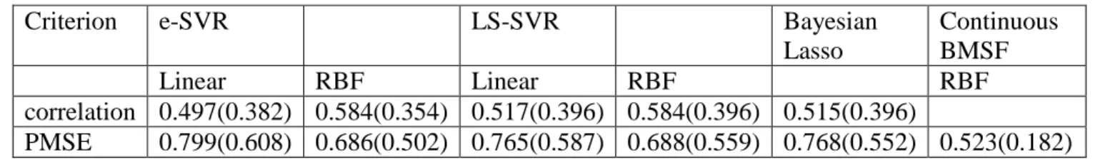
The results showed that by applying the continuous response version of BMSF method, we can obtain better prediction performance by building model on fewer genotyping markers. In Long et al. (2009), the wheat data was partitioned randomly into a training set (480 lines) and a test set (119 lines). Each time, two support vector regression models (Ɛ-SVR and LS-SVR) were applied directly to predict the wheat grain yield based on the genotyping markers from the training set, then the test data set was analyzed using the trained model to obtain predictive correlation and predictive mean squared error which were used to measure the predictive performance. For each method, a linear kernel and a Gaussian RBF kernel were compared. The best predictive performance was reached when using LS-SVR with a RBF kernel, in which case, the predictive correlation and mean squared error were 0.584 and 0.688 with the standard

deviation of 0.354 and 0.559 respectively. It is worth to mention that in Long et al. (2009), the standard errors of the mean squared error were given instead of standard deviation, and all the standard errors were calculated by building models 50 times based on random partitioned training-test data sets. In order to compare the result from Long et al. (2009) with the result of the continuous version of BMSF method, we calculated the standard deviations based on their reported standard errors multiplied by the square root of the times of training-test partitions. On the other hand, with the continuous version of BMSF method, we dramatically reduced the dimension of the data, and improved the predictive performance significantly. We used the same partition method to get the training and test sets and then applied the feature selection algorithm to the training data. The number of selected genes ranged from 27 to 50 with an average of 41 genes retained after the algorithm completed. We used the selected genes to build the Ɛ-SVR regression models to analyze the test data and obtained mean squared error to measure the predictive performance. We repeated this process on 10 random partitions of training and test

(23)

17

sets. The lowest and highest MSE were 0.3761 and 0.8898 respectively, with an average of 0.5228, and the standard deviation was 0.182. The details of the 10 runs of wheat data analysis are presented in the Appendix B in Table B.1. The summarized results of the wheat data analysis are presented in Table 4.1.

Table 4.1 Predictive correlations and predictive mean squared errors (PMSE) on the testing set by different methods: e-SVR, LS-SVR, Bayesian Lasso and Continuous BMSF.

Criterion e-SVR LS-SVR Bayesian

Lasso Continuous BMSF Linear RBF Linear RBF RBF correlation 0.497(0.382) 0.584(0.354) 0.517(0.396) 0.584(0.396) 0.515(0.396) PMSE 0.799(0.608) 0.686(0.502) 0.765(0.587) 0.688(0.559) 0.768(0.552) 0.523(0.182) Note: The mean values of e-SVR, LS-SVR and Bayesian Lasso were taken directly from Long et al. (2009). The

standard deviations of e-SVR, LS-SVR and Bayesian Lasso were calculated based on their reported standard errors multiplied by the square root of the times of training-test partitions. The standard deviations are given in

parentheses.

4.2 Continuous response version of the BMSF on simulated data

To further evaluate the continuous version BMSF algorithm in terms of the false selection rates, we conducted a simulation study. The data generation follows a model given in Fan et al. (2011). First, we define functions:

𝑔₁ 𝑥 = 𝑥, 𝑔₂ 𝑥 = 2𝑥 − 1 2_{, 𝑔}

3 𝑥 =

sin 2𝜋𝑥

2−sin 2𝜋𝑥 , and

𝑔₄ 𝑥 = 0.1 sin 2𝜋𝑥 + 0.2 cos 2𝜋𝑥 + 0.3 𝑠𝑖𝑛2_{2𝜋𝑥 + 0.4𝑐𝑜𝑠}3_{2𝜋𝑥 + 0.5𝑠𝑖𝑛}3_{2𝜋𝑥 .}

Then we generated the data from the additive model:

𝑌 = 3𝑔₁ 𝑋₁ + 3𝑔₂ 𝑋₂ + 2𝑔₃ 𝑋₃ + 2𝑔₄ 𝑋₄ + 𝐶 3.3843Ɛ ,

where the covariates 𝑋 = (𝑋₁, … , 𝑋_𝑝)𝑇_{are simulated according to the random-effects model} 𝑋𝑗 =

𝑊𝑗+𝑡𝑈

1+𝑡 , j=1,…,p, where 𝑊1, … , 𝑊𝑝and U are iid Unif(0,1), and Ɛ ~ N(0,1).

When t=0, the covariates are all independent, and when t = 1, the pairwise correlation of covariates is 0.5. Here C can take a series of different values to make the corresponding signal-to-noise ratio (SNR) vary. This is used to determine the difficulty of selecting individual variables.

(24)

18

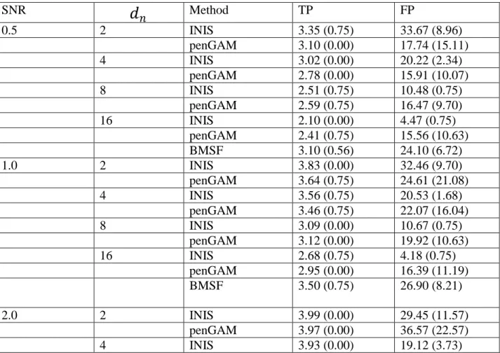
For our simulation, we set different SNR values to simulate data for evaluating the modified algorithm. In more details, for each SNR value 0.5, 1, 2, and 4, we generated 10 data sets with sample size of 100 (n=100) and applied the continuous version BMSF algorithm to each of the 10 sets of data to calculate the average true and false selection rates. The

corresponding C is 2 , 1, 0.5, and 0.5 respectively. For each of the simulation, we set p=1000 and t=1. The variable selection results on that simulated data set are presented in Table B.2. The summarized results are organized in Table 4.2. INIS and penGAM were two methods used in Fan et al. (2011) which are also included in Table 4.2 for comparison. The 𝑑_𝑛 in the table denotes the number of basis functions that are used to build the marginal nonparametric regression function. Smaller 𝑑_𝑛 is associated with smoother regression function.

Table 4.2 Average values of the numbers of TP, FP for different methods (INIS, penGAM, continuous version of BMSF) with different SNR and 𝒅_𝒏 values, robust standard deviations are given in parentheses. The INIS and penGAM results are based on sample size n=400 while those for BMSF are based on sample size n=100.

SNR

_𝑑

𝑛 Method TP FP 0.5 2 INIS 3.35 (0.75) 33.67 (8.96) penGAM 3.10 (0.00) 17.74 (15.11) 4 INIS 3.02 (0.00) 20.22 (2.34) penGAM 2.78 (0.00) 15.91 (10.07) 8 INIS 2.51 (0.75) 10.48 (0.75) penGAM 2.59 (0.75) 16.47 (9.70) 16 INIS 2.10 (0.00) 4.47 (0.75) penGAM 2.41 (0.75) 15.56 (10.63) BMSF 3.10 (0.56) 24.10 (6.72) 1.0 2 INIS 3.83 (0.00) 32.46 (9.70) penGAM 3.64 (0.75) 24.61 (21.08) 4 INIS 3.56 (0.75) 20.53 (1.68) penGAM 3.46 (0.75) 22.07 (16.04) 8 INIS 3.09 (0.00) 10.67 (0.75) penGAM 3.12 (0.00) 19.92 (10.63) 16 INIS 2.68 (0.75) 4.18 (0.75) penGAM 2.95 (0.00) 16.39 (11.19) BMSF 3.50 (0.75) 26.90 (8.21) 2.0 2 INIS 3.99 (0.00) 29.45 (11.57) penGAM 3.97 (0.00) 36.57 (22.57) 4 INIS 3.93 (0.00) 19.12 (3.73)

(25)

19 penGAM 3.91 (0.00) 31.31 (20.52) 8 INIS 3.50 (0.75) 10.29 (0.75) penGAM 3.71 (0.75) 27.06 (19.03) 16 INIS 2.93 (0.00) 4.07 (0.00) penGAM 3.22 (0.00) 19.51 (12.13) BMSF 3.70 (0.56) 31.40 (8.02) 4.0 2 INIS 4.00 (0.00) 29.47 (11.38) penGAM 4.00 (0.00) 37.27 (20.71) 4 INIS 3.99 (0.00) 17.36 (5.22) penGAM 4.00 (0.00) 38.71 (20.34) 8 INIS 3.78 (0.00) 10.00 (0.00) penGAM 3.99 (0.00) 41.42 (15.86) 16 INIS 3.02 (0.00) 3.98 (0.00) penGAM 3.72 (0.75) 29.58 (19.40) BMSF 3.90 (0.00) 31.10 (17.72)

Table 4.3 Significance tests between BMSF and other methods with different 𝐝_𝐧 under the same SNR value. Significant decisions are made based on Bonferroni correction at family-wise error rate 0.05. The results of whether or not the test is significant are given in

parentheses (N: not significantly different from BMSF, L: significantly lower than BMSF, H: significantly higher than BMSF).

SNR

_𝑑

𝑛 comparison with BMSF TP FP 0.5 2 INIS 0.2171(N) 0.001249(H) penGAM 1(N) 0.0242(N) 4 INIS 0.6621(N) 0.1021(N) penGAM 0.1042(N) 0.003868(L) 8 INIS 0.009365(N) 0.0001231(L) penGAM 0.02052(N) 0.006083(L) 16 INIS 0.0003148(L) 6.813e-06(L) penGAM 0.003514(L) 0.002936(L) BMSF 3.10 (0.56) 24.10 (6.72) 1.0 2 INIS 0.1975(N) 0.0686(N) penGAM 0.585(N) 0.5001(N) 4 INIS 0.8139(N) 0.03664(N) penGAM 0.8752(N) 0.1320(N) 8 INIS 0.1179(N) 0.0001488(L) penGAM 0.1436(N) 0.02819(N) 16 INIS 0.007223(N) 1.065e-05(L) penGAM 0.04556(N) 0.00271(L) BMSF 3.50 (0.75) 26.90 (8.21)

(26)

20 2.0 2 INIS 0.1359(N) 0.4965(N) penGAM 0.1617(N) 0.1393(N) 4 INIS 0.2263(N) 0.0008752(L) penGAM 0.2660(N) 0.9782(N) 8 INIS 0.3181(N) 1.599e-05(L) penGAM 0.9594(N) 0.1853(N) 16 INIS 0.001855(L) 1.914e-06(L) penGAM 0.02398(N) 0.0009049(L) BMSF 3.70 (0.56) 31.40 (8.02) 4.0 2 INIS NA(H) 0.7816(N) penGAM NA(H) 0.3227(N) 4 INIS NA(H) 0.03684(N) penGAM NA(H) 0.2269(N) 8 INIS NA(L) 0.004447(L) penGAM NA(H) 0.1054(N) 16 INIS NA(L) 0.0009213(L) penGAM 0.01826(N) 0.8023(N) BMSF 3.90 (0.00) 31.10 (17.72)

4.3 Discussion

From table 4.2, we can see that both methods evaluated in Fan et al. (2011) had very good true positive rate under various SNRs when the was not too large, and which turned worse when larger was used. On the other hand, both methods had the opposite tendency for false positive rate, that is, the FP was higher under smaller . For cross comparison, it is

reasonable to compare the result of BMSF with INIS and penGAM under the same SNR value in terms of TP and FP. We applied the two sample t test with confidence level of 0.95 between the results of BMSF and that of the other two with different under the same SNR value. Since we did eight significant tests for true positive rate or false positive rate of BMSF against that of other methods for each SNR value, the multiple comparison adjustment must be made. We applied Bonferroni correction to make the adjustment for the cutoff p-value. As a result, the cutoff p-value was equal to the selected confidence level divided by 8, which is 0.0065.The test results were summarized in table 4.3.

From table 4.3, for SNR = 0.5, the true positive rate of BMSF was not significantly different from that of INIS and penGAM when {2, 4, 8}, while it was better than the other two under = 16. And the false positive rate of BMSF was only better than that of INIS with

(27)

21

= 2 and was worse or not significantly different from that of INIS and penGAM with remaining values. The comparison results under SNR = 1 and SNR = 2 are very similar. Under SNR = 1, the true positive rate of BMSF was not significantly different from that of INIS and penGAM for all values; The false positive rate of BMSF was higher than that of INIS with = 8 and = 16 and penGAM with = 16, and was not significantly different from that of INIS and penGAM with the remaining values. And under SNR = 2, the result had a little difference such that the true positive rate of BMSF was higher than that of INIS with = 16 and the false positive rate of BMSF was higher than that of INIS with = 4. For SNR = 4, in terms of the true positive rate, BMSF did not perform as well as INIS or penGAM, except it was better than INIS with = 8, 16 and was not significantly different from penGAM with =16. For the false positive rate, the BMSF with n=100 performed not as good as INIS with n=400, = 8 and = 16, and there was no difference when compared it with penGAM under all values and INIS with = 2 and = 4.

In practice, for INIS and penGAM, it is difficult, if not impossible, to choose the best values for these methods to get the best TP and FP during the feature selection. The authors of INIS and penGAM did not offer insight on how to choose . We have seen that BMSF with n=100 has comparable performance to INIS and penGAM with n=400 for majority of settings. In very few settings under some values, INIS or penGAM had better results than BMSF.

(28)

22

Chapter 5 - Summary

In this report, we reviewed several statistical and machine learning methods for

Quantitative Trait Locus mapping and Genome-Wide Association Studies, most of which have been proved to be very successful in finding the QTL. However, in reality, the high dimension genomic data can be a nightmare for even the most successful method. Among these, support vector machine is the most common method used to deal with high dimensional problems, but it may still be painful if one uses it to analyze the high dimensional data directly. Instead, the feature selection method became a very important, if not necessary, technique which usually leads to better results. We reviewed the BMSF method by Zhang et al. (2012) originally

developed for binary response data taking into account the gene interactions in expression data. We modified BMSF so that it can be applied to continuous gene expression dataset. For the empirical study, we applied the continuous version of BMSF on some public data that has been analyzed using SVM method. The results showed that by applying feature selection before doing actual predictions we can get a much better result. To further evaluate the continuous version of BMSF, we did the simulation studies followed the data generation setting of Fan et al. (2011). In comparison to the smoothing based methods in Fan et al. (2011), the continuous version of BMSF showed good ability to identify active variables hidden among high dimensional irrelevant variables. In most of the comparison settings, BMSF with sample size n=100 had comparable performance to the INIS and penGAM with n=400.

(29)

23

Bibliography

The Wellcome Trust Case Control Consortium (2007). Genome-wide association study of 14000 cases of seven common diseases and 3000 shared controls. Nature, 447: 7.

Dίaz-Uriarte & Alvarez de Andre‟s (2006). Gene selection and classification of microarray data using random forest. BMC Bioinformatics, 7:3

Giorgio Guzzetta, Giuseppe Jurman & Cesare Furlanello (2009). A machine learning pipeline for quantitative phenotype prediction from genotype data. Machine Learning in

Computational Biology, 11: 53.

Jacob J Michaelson, Rudi Alberts, Klaus Schughart & Andreas Beyer (2010). Data-driven assessment of eQTL mapping methods. BMC Genomics, 11: 502.

http://www.biomedcentral.com/1471-2164/11/502.

Rita M. Cantor, Kenneth Lange, & Janet S. Sinsheimer (2010). Prioritizing GWAS Results: A Review of Statistical Methods and Recommendations for Their Application. The

American Journal of Human Genetics, 86 (1): 6–22.

Hongyan Zhang, Haiyan Wang, Zhijun Dai, Ming-shun Chen & Zheming Yuan (2012). Improving Accuracy for Cancer Classification with a New Algorithm for Genes Selection. To appear in BMC Bioinformatics.

Nanye Long, Daniel Gianola, Guilherme J. M. Rosa & Kent A. Weigel (2009). Application of support vector regression to genome-assisted prediction of quantitative traits. TAG

Theoretical and Applied Genetics,123: 1065-1074 .

Wei Zhou, Zhijun Dai, Yuan Chen, Haiyan Wang & Zheming Yuan (2012). High-Dimensional Descriptor Selection and Computational QSAR Modeling for Antitumor Activity of ARC-111 Analogues Based on Support Vector Regression (SVR). International Journal

(30)

24

Jianqing Fan, Yang Feng & Rui Song (2011). Nonparametric Independence Screening in Sparse Ultra-High-Dimensional Additive Models. Journal of the American Statistical

(31)

25

Appendix A - Codes and Implementations

A.1 Matlab code of Continuous response version of the BMSF

% Inputs:

% data: the first column is response variable(N by 1 categorical row vector, N is sample size),

% the remainder columns are independent variables(N by P matrix, P is gene number).

% iniMatrix_row: initial binary matrix rows to generate. eg: 500.

% step: rows reduction of generated binary matrix within rounds of feature selection. eg: 50. % lowerOfMatrix: the minimum rows of binary matrix to generate. eg: 300.

% cv_times: n-fold cross-validation, must >= 2.

% isScale: whether to scale the independent variables, 1 means scale, 0 means not. % libsvm_options: libsvm parameters, need a string variable. eg: ' -s 0 -t 2 '. % -s svm_type : set type of SVM (default 0)

% 0 -- C-SVC

% 1 -- nu-SVC

% 2 -- one-class SVM

% 3 -- epsilon-SVR

% 4 -- nu-SVR

% -t kernel_type : set type of kernel function (default 2)

% 0 -- linear: u'*v

% 1 -- polynomial: (gamma*u'*v + coef0)^degree % 2 -- radial basis function: exp(-gamma*|u-v|^2) % 3 -- sigmoid: tanh(gamma*u'*v + coef0)

% 4 -- precomputed kernel (kernel values in training_set_file) % Outputs:

% Filter_result: the process of feature selection.

% new_data : the response variable and final candidate genes. % screenProcess: the screening process of fine evaluation

% --- BMSF process --- for round=1:10, data = reshape(textread('simulated_data_SNR0.25_100_1.txt'),100,1001); iniMatrix_row = 160; step = 20; lowerOfMatrix = 100; cv_times = 5; isScale = 0; libsvm_options = ' -s 3 -t 2 ';

Filter_result = BinaryMatrixShufflingFilter(data, iniMatrix_row, step,lowerOfMatrix, cv_times, isScale, libsvm_options);

(32)

26 save(file);

% --- Fine evaluation --- fprintf('********** Fine evaluation of candidate genes. *************\n')

cv_mccs = cell2mat(Filter_result(2:end,4)); tmp = find(cv_mccs-min(cv_mccs)==0, 1, 'last' ); index = Filter_result{tmp+1,3}; Y = data(:,1); X = data(:,2:end); data2 = [Y X(:,index)];

[new_data, screenProcess] = fineEvaluation(data2, isScale, cv_times, libsvm_options); file=num2str([round round]);

save(file); end

function data_eval = BinaryMatrixShufflingFilter(data, iniMatrix_row, step, lowerOfMatrix, ... cv_times, isScale, libsvm_options)

%BinaryMatrixShufflingFilter Select features recursively using binary matrix shuffling filter. %

% data_eval = BinaryMatrixShufflingFilter(data_file, iniTable_row, Table_lower_threshold, Table_step, ...

% cv_times, isScale, libsvm_options) %

% The input parameters :

% data: the first column is an n-by-1 vector of response observations, the remainder columns is an n-by-p matrix, with rows

% corresponding to observations and columns to independent variables. % iniMatrix_row: initial binary matrix rows to generate.

% step: the rows reduction of generated Matrix former to latter filter round. % lowerOfMatrix: the minimum rows of binary matrix to generate.

% cv_times : n-fold cross-validation, must >= 2.

% isScale : whether to scale the data, 1 means scale, 0 means not. % libsvm_options : libsvm parameters, e.g:' -s 0 -t 2 '.

%

% The output parameter :

% data_eval : deleted and reserved descriptors information of each feature selection round. %

Y = data(:,1); X = data(:,2:end);

data_eval = {'round' 'deleted_x_index' 'reserved_x_index' 'CV_MCC' 'best_c' 'best_g'}; % ===================== get CV-MCC of initial data ====================

(33)

27 data_eval{2,1} = 'source_eval:';

temp_eval = libsvm([Y X], [], cv_times, isScale, libsvm_options); xIndex = 1:(size(X,2)); data_eval{2,3} = xIndex; data_eval(2,4:end) = num2cell(temp_eval); % ============================ filter descriptors ====================== former_eval = 0; cur_eval = 0; former_bestc = 0; cur_bestc = 0; del_x = 0; curMatrix_row = iniMatrix_row; m = 3; round = 1; RandStream.setDefaultStream(RandStream('mt19937ar','seed',sum(100*clock))); while ~isempty(del_x)

if cur_eval > former_eval && cur_bestc > former_bestc break

end

x_num = size(X,2);

binary_matrix = generate_binary_matrix(x_num, curMatrix_row);

eval_rlt = get_matrix_result(binary_matrix, [Y X], cv_times, isScale, libsvm_options); matrix_eval_rlt = [eval_rlt binary_matrix];

table_eval = matrix_eval_rlt(:,1);

if max(table_eval)~=min(table_eval) && (abs(mean(table_eval))<0 || abs(mean(table_eval))>1) table_eval = (table_eval-min(table_eval))/(max(table_eval)-min(table_eval)); end matrix_eval_rlt(:,1) = table_eval; replace_rlt = get_replace_rlt(matrix_eval_rlt, 10, ' -s 3 -t 2 -q '); del_x = get_del_x(replace_rlt, matrix_eval_rlt);

data_eval{m,1} = [num2str(round) '_round_eval:']; data_eval{m,2} = del_x;

xIndex(del_x) = []; data_eval{m,3} = xIndex; X(:,del_x) = [];

temp_eval = libsvm([Y X], [], cv_times, isScale, libsvm_options); data_eval(m,4:end) = num2cell(temp_eval);

(34)

28 former_eval = data_eval{m-1,4};

cur_eval = data_eval{m,4}; former_bestc = data_eval{m-1,5}; cur_bestc = data_eval{m,5};

fprintf(['###### %d(th) round of filtering has been completed, %d descriptors are deleted and ' ...

'%d descriptors are reserved in this round. ##########\n'], ... round, length(del_x), size(X,2))

% save FilterResultOfEachRound data_eval m = m+1; round = round+1;

if curMatrix_row-step >= lowerOfMatrix curMatrix_row = curMatrix_row - step; end

end

function rand_table = generate_binary_matrix(x_num, table_row) rand_table = nan(table_row, x_num);

fi = 0; while fi == 0 for n = 1:x_num rand12 = randperm(table_row); rand12(rand12<=length(rand12)/2) = 0; rand12(rand12>0) = 1; rand_table(:,n) = rand12'; end for m = 1:table_row if sum(rand_table(m,:)) == 0 fi = 0; break; else fi = 1; end end end rand_table(rand_table==0) = -1;

(35)

29

function eval_rlt = get_matrix_result(binary_matrix, data, cv_times, isScale, libsvm_options) data_y = data(:,1); data_x = data(:,2:end); binary_matrix_row = size(binary_matrix,1); for m = 1:binary_matrix_row temp = binary_matrix(m,:); del_x = temp==-1; new_x = data_x; new_x(:,del_x) = [];

eval_rlt(m,:) = libsvm([data_y new_x], [], cv_times, isScale, libsvm_options);

fprintf('Binary_matrix: %d(th) row, the corresponding CV-MCC is %g.\n', m, eval_rlt(m,1))

end

eval_rlt(:,2:end) = [];

function rlt = get_replace_rlt(train, cv_times, libsvm_options)

% ====================== parameter selection for libsvm =================== best_para = gridr(train, cv_times, libsvm_options);

bestc = best_para(2); bestg = best_para(3); bestp = best_para(4);

% ====================== training process ============================= options = [' -c ' num2str(bestc) ' -g ' num2str(bestg) ' -p ' num2str(bestp) ' ' libsvm_options]; model = svm_train(train(:,1), train(:,2:end), options);

train_row = size(train,1); train_col = size(train,2); % ====================== predicting process ============================= rlt1 = nan(train_row, (train_col-1)); rlt2 = nan(1, (train_col-1)); rlt3 = nan(1, (train_col-1)); % tic for m = 2:train_col test = train;

(36)

30 test(train(:,m)==1,m) = -1;

test(train(:,m)==-1,m) = 1;

rlt1(:,m-1) = svm_predict(test(:,1), test(:,2:end), model); test2 = train(1,:);

test2(2:end) = (max(train(1,2:end))+min(train(1,2:end)))/2; test2(m) = -1;

rlt2(m-1) = svm_predict(test2(1), test2(2:end), model); test2(m) = 1;

rlt3(m-1) = svm_predict(test2(1), test2(2:end), model);

% fprintf('The %d(th) descriptor has been replaced, elapsed time is %g seconds!!\n', m-1, toc) end

rlt4 = [rlt2 rlt3]; rlt = {rlt1 rlt4};

function best_para = grid(data, cv_times, libsvm_options) Y = data(:,1);

X = data(:,2:end); best_mcc = realmax; for log2c = -5:2:10 for log2g = 3:-2:-10

options = [' -c ' num2str(2^log2c) ' -g ' num2str(2^log2g) ' -v ' num2str(cv_times) ' ' libsvm_options];

mcc = svm_train(Y, X, options); if mcc < best_mcc

best_mcc = mcc; bestc = 2^log2c; bestg = 2^log2g; end

% fprintf('%g %g %g (best c=%g, g=%g, mcc=%g)\n', log2c, log2g, mcc, bestc, bestg, best_mcc);

end end

best_para = [best_mcc bestc bestg];

function best_para = gridr(data, cv_times, libsvm_options) Y = data(:,1);

X = data(:,2:end); best_mse = realmax; for log2c = -1:6 for log2g = 0:-1:-8

(37)

31 for log2p = -8:-1

options = [' -c ' num2str(2^log2c) ' -g ' num2str(2^log2g) ' -p ' num2str(2^log2p) ' -v ' num2str(cv_times) ' ' libsvm_options];

mse = svm_train(Y, X, options); if mse < best_mse

best_mse = mse; bestc = 2^log2c; bestg = 2^log2g; bestp=2^log2p; end

% fprintf('%g %g %g %g (best c=%g, g=%g, p=%g, mse=%g)\n', log2c, log2g, log2p, mse, bestc, bestg, bestp, best_mse);

end end end

best_para = [best_mse bestc bestg bestp];

function [accuracy, predict_label, best_para] = libsvm(train, test, cv_times, isScale, libsvm_options)

train_Y = train(:,1); train_X = train(:,2:end); if isScale

[train_X scale_range] = svm_scale(train_X); if ~isempty(test)

test_Y = test(:,1);

test_X = svm_scale(test(:,2:end), scale_range); end else if ~isempty(test) test_Y = test(:,1); test_X = test(:,2:end); end end % ================== parameter selection ==================== best_para = grid([train_Y train_X], cv_times, libsvm_options);

% ======= training process and predicting process =========== if ~isempty(test)

options = [' -c ' num2str(best_para(2)) ' -g ' num2str(best_para(3)) ' ' libsvm_options]; model = svm_train(train_Y, train_X, options);

[predict_label, accuracy] = svm_predict(test_Y, test_X, model); accuracy(2:end) = [];

(38)

32 accuracy = best_para;

end

function del_x = get_del_x(ud_replace_rlt, ud_result)

ud_Y = ud_result(:,1); ud_table = ud_result(:,2:end); x_num = size(ud_table,2); ud_Y = repmat(ud_Y,1,x_num); real1 = ud_replace_rlt{1}; real2 = ud_replace_rlt{1}; real1(ud_table==-1) = ud_Y(ud_table==-1); real2(ud_table==1) = ud_Y(ud_table==1); rlt1_mean = mean(real1,1); rlt2_mean = mean(real2,1); rlt3 = ud_replace_rlt{2}(:,1:x_num); rlt4 = ud_replace_rlt{2}(:,x_num+1:end); del_x1 = find(rlt1_mean < rlt2_mean); del_x2 = find(rlt3 < rlt4);

del_x = union(del_x1, del_x2);

function [new_data, screenProcess] = fineEvaluation(data, isScale, cv_times, libsvm_options) %FINEEVALUATION Fine evaluation of candidate genes retained from earlier filtering. %

% Inputs:

% data: the first column is an n-by-1 vector of response observations, the remainder columns is an n-by-p matrix, with rows

% corresponding to observations and columns to independent variables. % isScale : whether to scale the data, 1 means scale, 0 means not.

% cv_times : n-fold cross-validation, must >= 2. % libsvm_options : libsvm parameters, e.g:' -s 0 -t 2 '. %

% Outputs:

(39)

33

% screenProcess: the screening process of fine evaluation % Y=data(:,1); X=data(:,2:end); if cv_times == 0 cv_times = size(X,1); end

CVmcc0 = libsvm([Y X], [], cv_times, isScale, libsvm_options); CVmcc0 = CVmcc0(1); screenProcess=nan(size(X,2)-1,size(X,2)+2); jj=1; di=1:(size(data,2)-1); Xparmrk=1:size(X,2); while size(X,2)>1 parc=size(X,2);

fprintf('Cross-validation MCC with whole descriptors of this turn: %g\n',CVmcc0); screenProcess(jj,1)=CVmcc0; CVmcc_middle=nan(1,parc); i=1; for pari=1:parc cX=X; cX(:,pari)=[];

tmp = libsvm([Y cX], [], cv_times, isScale, libsvm_options); CVmcc_middle(pari) = tmp(1);

fprintf('Cross-validation MCC without descriptor #%g: %g\n',Xparmrk(pari),CVmcc_middle(pari)); if di(Xparmrk(pari))==0 i=i+1; else screenProcess(jj,di(Xparmrk(pari))+i)=CVmcc_middle(pari); end end [minCVmcc,minCVmccIndex]=min(CVmcc_middle); jj=jj+1; if minCVmcc<=CVmcc0

fprintf('Descriptor #%g has been washed out.\n',Xparmrk(minCVmccIndex)); screenProcess(jj-1,end)=Xparmrk(minCVmccIndex);

di(Xparmrk(minCVmccIndex))=0; X(:,minCVmccIndex)=[];

(40)

34 CVmcc0=minCVmcc;

else

disp('No any descriptor-deleting is necessary, screenning is finished.'); disp(['Remainder descriptor(s): ',sprintf('%g,',Xparmrk)]);

break end end

new_data = [data(:,1),X(:,:)];

A.2 R code for data simulation

t=1 n=100 p=1000 C=sqrt(0.25) unif=runif(n,min=0,max=1) U=matrix(unif,nrow=n,ncol=p) X=matrix(nrow=n,ncol=p) W=matrix(nrow=n,ncol=p) N=matrix(nrow=n,ncol=1) Y=matrix(nrow=n,ncol=1) for(i in 1:p){ W[,i]=matrix(runif(n,min=0,max=1)) } X=(W+t*U)/(1+t) g1=function(x){ return(x) } g2=function(x){ y=(2*x-1)^2 return(y)

(41)

35 } g3=function(x){ y=sin(2*pi*x)/(2-sin(2*pi*x)) return(y) } g4=function(x){ y=0.1*sin(2*pi*x)+0.2*cos(2*pi*x)+0.3*(sin(2*pi*x))^2+0.4*(cos(2*pi*x))^3+0.5*(sin( 2*pi*x))^3 return(y) } N=matrix(rnorm(n,mean=0,sd=1)) for(j in 1:n){ Y[j]=3*g1(X[j,1])+3*g2(X[j,2])+2*g3(X[j,3])+2*g4(X[j,4])+C*sqrt(3.3843)*N[j] } sdata=cbind(Y,X) write.table(sdata, file="D://dayoujiang//2011_second_half//ms_report_disease_mapping//bmsf//BMSF-March 07, 2012//simulation_SNR_0.25//simulated_data_SNR0.25_10.txt", row.names=FALSE, col.names=FALSE,append = FALSE,sep="\t",eol="\n")