Discussion Paper Series
Total Unit Costs, Marginal Costs and the New
Keynesian Phillips Curve
By
George Bratsiotis and Wayne Robinson
Centre for Growth and Business Cycle Research, Economic Studies,
University of Manchester, Manchester, M13 9PL, UK
September 2009
Number 123
Download paper from:
http://www.socialsciences.manchester.ac.uk/cgbcr/discussionpape
rs/index.html
Total Unit Costs, Marginal Costs and the
New Keynesian Phillips Curve
George J. Bratsiotis and Wayne A. Robinson
University of Manchester,
Centre for Growth and Business Cycle Research, (CGBCR),
This version: June 29, 2011
Abstract
The bulk of the literature that estimates the new Keynesian Phillips curve, (NKPC), uses unit labor costs as a proxy to marginal cost. This paper considers the contribution of non-labor unit costs to the latter. The theory-based marginal cost is derived as a function of both labor and non-labor unit costs, (including capital, net interest payments and tax related costs). Using data on labor and non-labor payments
in nonfarm GDP for the US, we constructtotal unit costs as our proxy for marginal cost. Total unit costs are shown to improve the …t of the short-run variation in in‡ation and strengthen the empirical support for the role of expectations-based in‡ation persistence and real mar-ginal cost as the driving variable in the NKPC. They also imply a duration of …xed nominal contracts that is closer to those suggested by …rm-level surveys, than that implied by unit labor costs alone.
JEL: E5, E31, E32, E37
Keywords: New Keynesian Phillips Curve; marginal cost proxies; in‡ation persistence; price rigidity duration.
Economics, School of Social Sciences, University of Manchester, Manchester M13 9PL, UK; Email: george.bratsiotis@manchester.ac.uk.
We thank Je¤ Fuhrer for sharing his program and Carl Walsh for very useful comments. We also thank John Fender, Christopher Martin, Paul Mizen, Hashem Pesaran, Denise Osborn, Keneth Wallis and Birmingham University Macro/Econometrics Conference 2009 participants; also Bhavani Khandrika and Michael Chernousov of the US Bureau of Labor Statistics and Tim Howells of the US Bureau of Economic Analysis for assistance with the data. Errors or the views in this paper remain our own.
Contents
1 Introduction 3
2 The Model 8
2.1 Households . . . 9
2.2 The Credit Market . . . 11
2.3 Wholesale and Intermediate Firms . . . 12
2.4 The New Keynesian Phillips Curve . . . 15
2.5 Monetary Policy and Macro Equilibrium . . . 17
3 Empirical Estimation 18 3.1 Data . . . 18
3.2 Structural Estimates . . . 21
3.2.1 Total Unit Costs and Forward Looking Behavior . . . . 23
3.2.2 Actual versus Fundamental In‡ation . . . 26
3.3 Total Unit Costs and In‡ation Persistence . . . 27
4 Concluding Remarks 29
References 30
1
Introduction
Largely inspired by Gali and Gertler (1999), the New Keynesian Phillips Curve (NKPC) has emerged as a key feature of many dynamic macroeco-nomic models and a key tool in monetary policy analysis. In spite of its recent popularity however, there is still an ongoing debate as to whether the NKPC can match the observed in‡ation persistence and the length of …xed nominal price contracts as implied by surveys at the micro level. Accumu-lating empirical evidence on the performance of the NKPC suggests that in explaining the dynamics of in‡ation, (a) real marginal cost is a better driving variable than the output gap, and (b) the hybrid NKPC, that includes lagged in‡ation, performs empirically better than the purely forward looking NKPC. This has led to a wide adoption of the hybrid NKPC which speci…es in‡ation as a function of lagged in‡ation, expected future in‡ation (one period ahead) and real marginal cost as the driving variable (see eq. 1, Gali, Gertler and Lopez-Salido 2005),
t= b t 1+ fEt t+1+ mcct+ t;
where t is the in‡ation rate, mcct is real marginal cost (as a percentage
deviation from its steady state value) and t is a cost push shock. Gali and
Gertler (1999), Gali, Gertler and Lopez-Salido (2001, 2005) and Sbordone (2002, 2005) suggest only a “modest” role for intrinsic in‡ation persistence ( b); whereas others …nd a very limited role for forward looking expected
in‡ation ( f) in the NKPC, (see Fuhrer 1997 Rudd and Whelan 2005, 2007,
Lindé 2005, Lawless and Whelan 2007 among others).1 A common feature 1In a recent study, Zhang, Osborn and Kim (2008) show that forward-looking behavior
played a small role during the higher in‡ation volatility period 1968-1981 in the US, suggesting that during periods of high in‡ation volatility, in‡ation persistence in the NKPC may become more intrinsic.
in these studies is that when the coe¢ cient of marginal costs ( ) becomes more signi…cant the NKPC tends to become more forward looking. This is consistent with the theoretical concept that if in‡ation dynamics are not intrinsic to the model but driven largely by marginal costs, then expectations about future prices should matter more.2
Following Gali and Gertler (1999), real marginal cost in the NKPC is usually proxied byreal unit labor costs, where the latter is measured in rela-tion to the deviarela-tion of labor income share in the non-farm business sector from its mean. Until recently, little attention has been placed on the exact contribution of unit labor cost as a proxy to marginal costs. Fuhrer (2006) shows that most of the persistence found in US in‡ation data appears to be
intrinsic from the lagged in‡ation term in the NKPC and thus cannot be attributed to the conventional driving variable in these model, (i.e. the real marginal cost proxied by unit labor costs).
The potential weakness of using unit labor costs as a proxy for marginal cost is suggested by two observations in recent studies. First, the degree of and the shifts in persistence using this proxy are not consistent with those in in‡ation (see Fuhrer 2006). Second, the estimated coe¢ cient of the real marginal cost implies price rigidities that are not consistent with micro ev-idence. The size of this coe¢ cient in the empirical literature for the US is typically between 0.01 and 0.02, which assuming that the rate of discount is between 0.9 and 1.0, implies that the degree of price stickiness ranges be-tween 0.8 and 1; this implies a duration of price contracts of 6 quarters or much longer. This is inconsistent with a number of …rm-level surveys which suggest that price rigidity ranges between 1.5 to 4 quarters.3 These two
ob-2We discuss this further in section 2.
3See Blinder, Canetti, Lebow and Rudd (1998), Hall, Walsh and Yates (2000),
servations suggest that labor unit costs may be a weak proxy to marginal costs, (see Rudd and Whelan 2002, 2007, Lindé 2005). Rudd and Whelan (2002) show that the labor share version of the NKPC explains a very small proportion of the variation in in‡ation. Lawless and Whelan (2007) use both sectoral and aggregate data from 1979-2001 for all EU-15 countries and the US. They test for both reduced form and structural speci…cations of in‡ation and …nd negative coe¢ cients on the e¤ect of the labor share on in‡ation.4
They conclude that the NKPC joint prediction of in‡ation and labor share cannot explain the trends in the data, particularly at the sectoral level. Ear-lier, Rotemberg and Woodford (1999) provided evidence that labor income share is a weak proxy for marginal cost in the US and suggest incorporating labor adjustment costs in order to generate more procyclical marginal costs. However, Sbordone (2005) shows that augmenting the marginal cost proxy, by incorporating adjustment costs, does not signi…cantly improve the …t of the NKPC for US data.
Following Wolman (1999), who suggests that more re…ned estimates of marginal costs should be investigated, a recent strand in the literature ex-amines whether alternative marginal cost proxies can improve the …t of the NKPC.5The bulk of this literature assumes di¤erent production technologies
(2004), Gwin and VanHoose (2007), Coenen, Levin and Kai (2007) and Rotemberg and Woodford (1997).
4Lawless and Whelan (2007) also provide evidence that although there has been a
widespread decline in labor shares across a broad range of sectors, these declines have not been associated with large shifts in in‡ation, indicating that labor share may be an incorrect proxy for marginal cost in estimating the NKPC.
5Some studies focus directly on re…ning proxies for the output gap. For example, using
di¤erent approaches, Chadha, and Nolan (2004), Neiss and Nelson (2005), and Bjørnland, Leitemo and Maih (2009) show that the use of theory consistent output gaps can be as good a proxy as real marginal cost. They suggest that the output gap proxies may not perform as well because output trends, that are largely used in the literature, are poor approximations to the output gap.
and aggregation methods and express average marginal cost as a function of both labor unit costs and the output (or employment) gap (Sbordone 2002, 2005, Gagnon and Khan 2005, Matheron and Maury 2004).6 This literature
concludes that assumptions about the nature of the production technology and aggregation factors may improve the …t of the NKPC, though this is sub-ject to the production technology parameters assumed. More recently, Gwin and VanHoose (2007, 2008) examine alternative measures of marginal cost and prices in estimating the NKPC. 7 The key contribution in their papers comes from the use of a PPI-in‡ation measure, which is shown to produce signi…cantly di¤erent results to those implied by Gali and Gertler. However, in using their alternative marginal cost data to replicate the tests by Gali and Gertler (1999), they too conclude that their estimates do not di¤er from what has already been shown in the literature (Gwin and VanHoose 2008).
Building on these recent …ndings, this paper shows that the inclusion of non-labor unit costs in the marginal cost proxy helps improve the …t of the short-run variation in in‡ation. We show that the theory-consistent real marginal cost implies that not only changes in labor unit costs but also in non-labor costs, such as capital unit costs, (accounting for capital utilization and depreciation), net …nance costs (i.e. net interest payments related to the …rm’s borrowing costs and …nancial assets) and production taxes, can determine the variation in the in‡ation-output trade o¤. Available aggregate
6These studies assume that capital does not change with respect to changes in the
relative price of …rms, hence the resulting real marginal cost is still largely driven by labor unit costs, as assumed in Gali and Gertler (1999).
7They develop a measure of average variable costs using Standard & Poor’s Compustat
database for publicly traded U.S. companies.This comprises …nancial data from quarterly and annual Securities and Exchange Commission …lings by over 10,000 …rms. From this database they obtain individual …rm revenues and costs of goods sold for the period 1966:1-2004:4 and construct a PPI and a growth rate of average variable costs as proxies to average price and marginal costs, respectively.
data that closely match our description of non-labor costs appear to be the
non-labor paymentsin nonfarm GDP as published by the US Bureau of Labor Statistics (BLS) and the U.S. Department of Commerce Bureau of Economic Analysis. Proportionally, non-labor payments are much smaller than labor payments, however, as …gure 1 shows the variation in non-labor payments is substantially large, suggesting that this component may be an important source of variation in marginal costs in the short run.8
{Figure 1. 12-mth Change in Proxies for Real Marginal Cost}
Using the above data we construct our real marginal cost proxy,total unit costs, as the sum of the shares of labor unit costs and non-labor unit costs of all nonfarm business sector in nonfarm GDP, de‡ated by the non-farm de‡ator.9 We show that the addition of non-labor unit costs to the widely
used unit labor costs, improves on the existing empirical support for the role of real marginal cost as the driving variable in the NKPC. In particular, by replicating the methodology of Gali and Gertler (1999) and Gali, Gertler and Lopez-Salido (2005), using non-linear GMM estimates on US data for the sample period 1966:Q1 to 2003:Q4, we …nd that whereas real unit labor costs, as a proxy to marginal cost, produce a coe¢ cient of around0:02, for the same sample period and methodology the equivalent coe¢ cient for total unit costs is around0:05or higher. The use oftotal units costs as a marginal cost proxy is also shown to increase the importance of the forward looking or
expectations-based in‡ation persistence f; this e¤ect is stronger in periods
8See also …gures 1a and 1b below
9Given the homogeneity in the data source, (US, BLS) we see this as the most natural
extension to the already familiar unit labor costs employed widely in the literature. Further details on the de…nition and construction of total unit costs are given in the empirical section below.
of relatively higher in‡ation volatility, rather than in the more recent years of in‡ation stability. Our results also suggest that total unit costs imply a duration of …xed nominal contracts of around 4 quarters or less, which is much closer to the …rm-level surveys based on micro data (1.5 to 4 quarters), than that implied purely by labor unit costs, (i.e. around 5-6 quarters or higher).
The remaining paper is structured as follows. Section 2 sets out the theoretical model which consists of households, a credit market, wholesale and intermediate …rms and a monetary authority; from the former sectors we derive the NKPC where non-labor costs are shown to enter the de…nition of marginal cost. Section 3 discusses the data followed by estimates of the NKPC and fundamental in‡ation. Section 4 concludes and discusses the implications of the main results.
2
The Model
We consider a dynamic stochastic general equilibrium model describing an economy that consists of households, wholesale and intermediate …rms, a credit market and a central bank. Households own capital and provide their labor and capital rental services to …rms. Wholesale …rms use intermediate goods to produce a …nal good that is traded competitively. Intermediate …rms compete monopolistically; they determine the demand for labor and capital and set prices, but they need to borrow from the credit market to cover their variable costs (wages and rental cost of capital). Firms also hold some safe assets for collateral purposes. The credit market receives deposits from households and provides loans to …rms. Given the loan rate determined by banks, …rms decide on the demand for loans whereas the supply of loans
is determined elastically at the loan rate; we assume that the credit market makes normal pro…ts which together with the pro…ts of …rms are distributed back to households.
2.1
Households
Households are represented by a typical agent who provides a homogenous labor service,n, to all producing …rms, derives utility from holding cash,Mt,
for transactions purposes and consumes a basket of all produced goods, ct.
Households maximize their expected present discounted value utility,10
Et 1 X s=0 s ( c(1t+s ) 1 + m 1 Mt+s Pt+s 1 nn 1+ t+s 1 + ) ; (1)
where < 1 is the subjective discount factor; ; m; n are elasticities;
= 1= is the marginal disutility of labor and the labor supply elasticity. Households nominal income consists of, cash endowmentsMt 1; gross interest
payments on deposits from the previous period, Dt 1, where RDt = (1 +iDt )
andiD
t is the nominal deposit rate; wage income,PtwtNt, wherewtis the real
wage rate; capital rental income, rtutkt, from letting their capital to …rms,
where rt is the real rental price of capital, kt, and ut is capital utilization;
and …nally, end of period (net of production tax) pro…ts from all …rms and the commercial bank,Vt=
R
Vj;t +Vtb, plus lump nominal sum transfersPt t.
The household’s budget constraint is,
Pt(ct+it) +Mt+Dt (2)
=Pt(wtnt+rtutkt) +Mt 1+RDt 1Dt 1 +Vt+Pt t
10Throughout the paper small latin letters,x, indicate real variables ofX, (apart from
the nominal interest rates,iX) whereasbxdenotes the log-linearised value ofxas a deviation
We assume that investment, it, is related to the capital stock as follows, it =kt+1 (1 (ut))kt+ kt+1 kt kt+1 (3) where (ut) = u't; 0
(u) > 0 is a depreciation function and kt+1
kt =
b
2(
kt+1
kt 1)
2 are quadratic costs related to capital investment;' is the
elas-ticity of marginal depreciation cost and so given 0( ) > 0, more capital utilization and higher values of' increases the rate of depreciation and thus capital consumption, (see Neiss and Pappa 2005).
Assuming no Ponzi-game conditions for all assets, and denoting the La-grangian multiplier of the budget constraint as t, the household’s …rst order
conditions are, ct = tPt (4) ct = Et PtRDt ct+1 Pt+1 (5) tPtwt = nnt (6) Mt Pt = Ct m RtD 1 RD t 1= (7) rt= 'u't 1 (8) Pt t 1 +b kt+1 kt 1 (9) = EtPt+1 t+1 " rt+1ut+1+ (1 u't+1) + b 2 kt+2 kt+1 2 1 !#
Equation (4) and (5) determine the marginal utility of consumption and Euler equation, while equations (6)-(9) de…ne the optimal allocations of labor, real balances and capital.
2.2
The Credit Market
The credit market is represented by a typical commercial bank, b. The bank accepts deposits from households, Dt, at the rate iDt , and makes loans, Lt,
to …rms at the loan rate iL
t. The demand for loans is determined by …rms
whereas the bank sets the interest rate on loans. If the credit market is short of liquidity, it can borrow from the central bank, LCBt at the re…nance (policy) rate, iCB
t . We assume that banks do not have to meet a reserve
requirement ratio. The commercial bank’s balance sheet is
Lt=Dt+LCBt (10)
We assume that in their conduct of intermediation commercial banks also in-cur some costs, t( t; yt); these are increasing in costs related to credit market
imperfections ( t), but decreasing with aggregate economic activity and will-ingness of banks to lend. In particular, we assume that t( t; yt) = t+yt ,
where >0, and tevolves as follows,log( t) = log( )+(1 ) log( t 1)+
;t. Thus at the steady state = log( ) = > 0, which captures the
mark-up over the policy rate due to market structure imperfections in the credit market, whereas ;t captures innovations to such costs, (for a similar
approach see Cook 1999, Atta-Mensah and Dib 2008).11The bank’s period pro…t function is,
Vtb =iLtLt iDt Dt iCBt L CB
t t( t; yt)Lt (11)
From (10), (11) and the above information and assuming normal pro…ts we derive,
iDt =iCBt and iLt =iCBt + t+yt ; (12)
11As shown below, this assumption also ensures that loan spreads are countercyclical,
as supported by empirical evidence. For a paper where such a relationship is explained endogenously see Agénor, Bratsiotis and Pfajfar, (2011).
hence with a zero requirement reserve ratio the deposit rate is equal to the re…nance rate whereas the loan rate is a mark-up over the re…nance rate driven by intermediation costs.
2.3
Wholesale and Intermediate Firms
There is a continuum of imperfectly competitive …rms,j 2[0;1], each engag-ing in the production of a di¤erentiated good, yj;t, which sells at the price
Pj;t: The …nal goods …rm bundles intermediate goods in a composite …nal
good yt= R1 0 y ( 1)= j;t dj =( 1)
, by minimizing the cost, Ptyt=
R1
0 Pj;tyj;tdj.
The resulting demand for each intermediate di¤erentiated good is, yj;t =
Pj;t
Pt
yt; (13)
where Pt is the average price index,
Pt= Z 1 0 Pj;t1 dj 1=(1 ) : (14)
The production of each intermediate good combines capital and labor ac-cording to the following CES technology,
yj;t = [ k(utkt) + n(atnt) ]
1=
; (15)
where = 1; 0 < k, n < 1 are the corresponding input shares and at
measures labor productivity. If = 0; equation (15) reduces to a standard Cobb-Douglas production function. The reason for deviating here from the widely used (in this literature) Cobb-Douglas production function, is that the latter assumes a unity elasticity of output with respect to labor and as a result the marginal cost is proportional to the labor share, (see Rotemberg and Woodford, 1999). The use of a CES production function allows the
marginal product of labor and hence marginal cost to be a¤ected by varying input shares hence this speci…cation is more appropriate for the purpose of this paper. Note, for simplicity, we assume that employment and capital is common to all …rms, which simpli…es aggregation while still allowing for the average and marginal products to vary, (see Gali, Gertler and Lopez-Salido, 2007, Cantore Levine and Yang, 2010).12
In each period intermediate …rms must borrow to cover their variable input costs (capital and labor), but they are required by lenders to hold some risk-free …nancial assets for risk diversi…cation and collateral purposes. In this paper the latter assumption serves mainly to capture the fact that many …rms tend to hold safe assets in their …nancial portfolio (i.e. for risk hedging, pension plans etc.). This implies that in addition to the borrowing costs, …rms also have a source of …nancial returns, which here we need in order to capture the item "net interest and miscellaneous payments" in the additional non-labor payments data used for constructing our total unit cost de…nition of marginal cost below.13 For simplicity we assume that all risk-free assets held by each …rm are summarized in the form of government bonds, Bj;t.14
Hence, the existing stock of all government bonds satis…es, Bt=
R1
0 Bj;tdj.
15
12Note that assuming …rm speci…c factor inputs within a CES production technology,
implies further relative price and in‡ation e¤ects as the marginal products of labor and capital are aslo a¤ected by the relative price and market power of the …rm. Gagnon and Khan (2005) examine such e¤ects in a model of labor input and …xed capital.
13For the exact data de…nitions see in the Appendix.
14Note that issues of risk and probability of default are not essential for the purpose
of this paper; for recent papers that deal with idiosyncratic risk see Faia and Monacelli (2007) and Agénor, Bratsiotis, and Pfajfar, (2011).
15Note that households and commercial banks could also hold government bonds, but
for the purpose of this paper we focus on bonds being held only by …rms. Within our framework this can be explained by the fact that bonds and deposits bear the same interest, hence the household treats them as very close substitutes. Similarly, given the two assets have the same return, (and given that commercial banks banks do not bear risk in this model), banks would rather use all deposits for loans rather than hold bonds. This however is not true for …rms which by assumption are required by banks to back part of their loans
Firms contract labor and capital at their market determined real wage and real rental price of capital, hence the …rm’s loan is equivalent to its variable cost,
Lt=Ptrtkt+Ptwtnt; (16)
We assume that a portion # of loans is collateralized by the …rm’s holdings of safe assets (before interest payments),16
#Lt=Bj;t (17)
From (15), 16 and (17), the …rm’s period pro…ts are, Vj;t =Pj;tyj;t(1 Yt ) +i
CB
t Bj;t RLtLt (18)
where, Y
t is a net (i.e. less subsidies or business transfers) production tax,
and RLt = 1 +iLt. Using (13)-(18), the period optimal real price of …rmj is,
Pj;t=Pt= pmct (19)
where p = =( 1) is the price mark-up and real marginal cost is,17
mct= 1 +iLt #iCBt 1 Y t rt kut(yt=kt)1 + wt nat(yt=nt)1 ; (20)
where kut(yt=kt)1 is the marginal product of capital and nat(yt=nt)1
is the marginal product of labor. With a Cobb-Douglas speci…cation, (i.e. with = 0), and with only labor costs, (where n = 1 ), (20) reduces
to mct = (1 )(wtyt=nt); which is the widely used marginal cost proxy, known
by collateral, i.e. bonds here.
16In Goodfriend and McCallum, (2007), loan makers construct collateral from
goveren-ment bonds and …rms’capital; Hnatkovska, Lahiri and Vegh, (2008) show borrowing …rms to have government bonds explicitly in their ‡ow constraint.
as the share of unit labor costs in GDP, (Gali, Gertler and Salido-Lopez 2001, 2005, Gali and Gertler 1999). However, from (20), real marginal cost here is a function of both unit labor costs and non-labor unit costs, the sum of which we de…ne as total unit cost in this paper. Unit labor costs is the familiar proxy as identi…ed elsewhere in the literature, whereasnon-labor unit costs, (in combination with (4)-(9) and (12)), are a function of, real capital costs, (accounting for capital consumption and depreciation); net interest payments that relate to the …rm’s borrowing costs and …nancial returns;
intermediations costs; and …nallynet production taxes.18
2.4
The New Keynesian Phillips Curve
We allow nominal rigidity to be characterized by a Calvo type price setting, according to which the price of each …rm has a …xed probability, , of re-maining …xed at the previous period’s price and a …xed probability of 1
of being adjusted. Each …rm setting a new price at time t will choose a price contract, Xt, to minimize current and future deviations of prices from
optimal prices, Pj;t+s, Et 1 X s=0 s t;t+s Pj;t Pj;t+s 2 ; (21)
where, t;t+s = sct+s=ct , is the discount factor. Minimizing (21) with
respect to Pj;t and denoting percentage deviations around a zero in‡ation
18Note that (20) is consistent with a some papers in the literature that derive marginal
costs as a function of labor costs as well as capital costs, borrowing costs and productions taxes, or combinations of these (see Christiano, Eichenbaum and Evans, 2001, Woodford, M. 2001, Ravenna and Walsh 2006, Chowdhury, Ho¤mann, and Schabert, 2006, Faia and Monacelli 2007, Di Bartolomeo, and Manzo, 2007, Agenor, Bratsiotis and Pfajfar 2011).
steady state by a hat, we obtain, b Xt = (1 ) 1 X s=0 s sE tPbj;t+s; (22) = (1 )(Pbj;t) + EtXbt+s;
where Xbt is the optimal price contract chosen by all …rms that adjust prices
in each period t and Pbj;t = Pbt+mcct is the optimal price based on (19),
approximated around a zero in‡ation steady state. The average price in the economy is,
b
Pt= Pbt 1+ (1 )PbtN; (23)
where newly set prices, PbN
t = (1 !)Xbt+!PbtB, are a weighted average of
optimally set prices,Xbtand backward looking set price,PbtB =Xbt 1+ t 1, (as
in Gali and Gertler, 1999). Using equations (22) and (23) and the de…nitions,
t=Pbt Pbt 1, t 1 =Pbt 1 Pbt 2 and Et t+1 =Et(Pbt+1 Pbt)we derive the
hybrid NKPC.
t= b t 1+ fEt t+1+ mcct; (24)
where, b = +!(1 !(1 )); f = +!(1 (1 )); = (1 +!!)(1(1 )(1(1 )));and the log-linearized marginal cost, or total unit costs, is19
c mct= iL^{L t #iCB^{CBt 1 +iL #iCB + SkSbk;t+SnSbn;t Sk+Sn + YbY t (1 Y); where,Sbk;t = ^rt (1 )(byt ^kt) u^t and Sbn;t = ^wt (1 )(^yt ^nt) bat,
are the shares of capital unit costs and labor unit costs respectively and Sk = r
k
k(y=k)(1 ) and Sn =
w
n(y=n)(1 ), are their respective steady states.
The log-linearized loan rate is,20 ^{Lt = i CB iL ^{ CB t + iLbt iLybt, where,^{CB
t is described in (25) below andbt= (1 )bt 1+ ;t:
From the coe¢ cients b, f, and , (24) implies that for any given proba-bility of …rms not adjusting prices ( ), a smaller weight on backward looking in‡ation (!) reduces the coe¢ cient on past in‡ation ( b), while increasing
the coe¢ cient on marginal costs ( ) and future expected in‡ation ( f); in which case the role of real marginal cost, as opposed to that of intrinsic in-‡ation, should also become more signi…cant in driving in‡ation dynamics in the model. Note that (24) is similar to the hybrid NKPC derived in Gali and Gertler (1999) and Gali, Gertler and Salido-Lopez (2001, 2005), with the main di¤erence being the composition of the real marginal cost; in the latter two studies, as with the bulk of the literature, marginal cost is proxied simply by unit labor costs, mcct= Sbn;t= ^wt (^yt n^t).
2.5
Monetary Policy and Macro Equilibrium
We complete the theoretical model by assuming that monetary policy is conducted by a Taylor-type interest rate rule; expressed in terms of deviations from steady state,
biCBt = ibiCBt 1+ (1 i) t+ ybyt + i;t (25)
where, 0 < i <1 and ; > 0 and i;t follows an AR(1) process. We
as-sume that any liquidity o¤ered by central banks as loans to the commercial
20At the steady state,iCB = 1
;iL=iCB+ , ( >0), and alsoa=u= 1;(see Neiss
bank enters through exogenous cash injections, (i.e. LCB
t = Mt Mt 1).21
We also assume that at the end of each period, any proceeds from produc-tion taxes, or from the central bank’s cash loans to the commercial bank, are transferred to households through a lump sum transfer, Pt t. Hence
equilibrium in the …nal goods markets must satisfy the aggregate resource constraint, yt =ct+it.
3
Empirical Estimation
In this section we replicate some of the key tests performed in the literature to show that, as indicated by the theoretical model, total unit costs is a more appropriate proxy for marginal cost than unit labor costs. We show that although unit-labor costs is the largest component of marginal cost, the addition of non-labor costs to the conventional labor unit costs adds more information to the data and improves the …t of in‡ation persistence and the proxy for real marginal cost as the driving variable in the NKPC.
3.1
Data
Our choice of data and its source remains as consistent as possible to the data already used in the literature. Total unit costs are constructed using quarterly data for labor costs and non-labor costs for the period 1966:Q1 to 2003:Q4, available from the US Bureau of Labor Statistics (BLS) and the U.S. Department of Commerce Bureau of Economic Analysis.22 Of these, la-21This, in conjuction with the bank’s balance sheet (equations 8 and 9), also de…ne the
demand for deposits, (see also Ravenna and Walsh, 2006).
22This sample period corresponds to Fuhrer (2006) as we want to compare our results
with those produced by Fuhrer’s ACF graph, (see Figure 4 below). Also, it is important here to emphasize that ourtotal unit costsis constructed from allnon-farm business sector
bor costs are the same data as that used widely in the literature.23 Non-labor
costs,are based onnon-labor payments (non-farm) as published by the BLS, less corporate pro…ts (non-farm). Thus, consistent with our theoretical spec-i…cation non-labor costs consist of, consumption of …xed capital, net taxes on production (and imports), net interest and miscellaneous payments (includ-ing borrow(includ-ing costs and interest earn(includ-ings on …nancial assets) and business current transfer payments.24 Our proxy for real marginal cost, realtotal unit
costs, is then constructed as the (log of) the sum oflabor costs andnon-labor costs in non-farm GDP, de‡ated by the (log of) non-farm de‡ator.25 As with
the rest of the literature, marginal cost is measured as a deviation from its mean, that is also consistent with the log-linearized theoretical model.
{Figure 2a} {Figure 2b}
Figures 2a and 2b compare annual in‡ation with the annual change in (non-farm)unit labor cost and (non-farm)total unit costs, respectively. Evidently, both unit labor costs and unit total costs track in‡ation, however the variance set we use is also clearly di¤erent to that used in Gwin and VanHoose (2007, 2008) that is constructed based on around 10,000 listed …rms in S&P, that is part of the six-digit NAICS industry classi…cations system.
23For more details see in the Appendix.
24As shown from (20)and (24) our theoretical marginal cost captures most of the key
components of the de…nition of the non-labor payments as given by the BLS, except import taxes. Had we assumed that part of the intermediate goods were imported, the marginal costs would also be a function of imported goods and hence import taxes. For comparative reasons, but also to keep our paper consistent with the bulk of the theoretical literature, we choose not to explore related theoretical issues of an open economy, although we recognize the importance of the latter. For a recent paper that considers open economy issues within a new Keynesian framework, see Adolfson, Laséen, Lindé, and Villani, (2005).
25Note that as indicated by a number of studies, the results do not di¤er much when
the all-sector GDP de‡ator is used instead of the non-farm GDP de‡ator (see Gali and Gertler 1999, Fuhrer 2006). Also, the use of the GDP de‡ator, as opposed to the PPI as suggested by Gwin and VanHoose (2007, 2008), is mainly for transparency in assessing the signi…cance of our marginal cost proxy in relation to the conventional estimations of the NKPC.
of unit total costs around in‡ation appears to be smaller than that of unit labor costs.26
Figures 3a-3d present, as a crude measure of persistence, the sample au-tocorrelations of the total unit cost and unit labor cost measures of marginal cost and in‡ation. For completeness, we also show the autocorrelation for
non-labor unit costs, the additional component of total unit costs. Figure 3a shows that the persistence in in‡ation is much greater than the persistence of unit labor costs. After the …rst four periods the autocorrelation in unit labor costs drops substantially in relation to that of actual in‡ation, whereas the opposite is shown for the persistence of the non-unit labor costs. As a result the combination of these two, that is the persistence in total unit costs, is shown to be much closer to the persistence in actual in‡ation.
{Figure 3a} {Figure 3b} {Figure 3c} {Figure 3d}
Empirical evidence suggests that most notable shifts in in‡ation persistence in the US occurred in the early 1980s and in the 1990s. Accordingly, in …gures 3b to 3d we plot the sample autocorrelations of the two alternative marginal cost proxies, for the sub-samples 1980-2003 and 1990-2003. Only non-labor unit cost and total unit cost show any perceptible shift in persistence across the samples.27The estimated sum of the lag coe¢ cients in a univariate
au-toregression over the full sample for unit labor cost, non-labor unit cost and total unit costs are 0.90, 0.97 and 0.95, respectively. However it is known
26Note the di¤erences in the height of the peaks of total unit costs (which is about 0.02
for the …rst shock and 0.01 at the second shock) re‡ect the response of non-labor costs to the oil price shock.
27A graph similar to …g 3b in our paper is in Fuhrer 2006, (page 74), that accounts only
that in the presence of shifts in persistence these estimates could be biased.
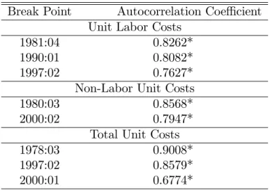
{Table 1: Test for Break Points in the Persistence of...}
Table 1 presents the results of a more formal estimation of persistence in the presence of unknown breaks (as suggested by Perron and Vogelsang 1992). Table 1 shows the break points and the coe¢ cients on the AR term for each resulting sub-sample. The changes in the size of the AR coe¢ cients are relatively small for unit labor costs thus con…rming the previous inference of very little change in persistence. The average of the AR coe¢ cients for non-unit labor costs and total non-unit costs are higher than the average for non-unit labor cost even after we account for the breaks. However, as Rotemberg (2007) demonstrates, the NKPC can generate in‡ation that is more persistent than the driving variable. Hence, one cannot rely on the univariate estimates of persistence in assessing alternative measures of marginal cost. In what follows therefore we turn to examine the structural estimates of the NKPC.
3.2
Structural Estimates
In this section we estimate the hybrid NKPC, equation (24), using non-linear instrumental variables (GMM) with robust errors over the period 1966:Q1 to 2003:Q4. To deal with the small sample normalization problem we follow Gali and Gertler (1999) and use the following orthogonality conditions,
Et 1f( t mcct f t+1 b t 1)zt 1g= 0 (26)
Et 1f( t (1 !)(1 )(1 )mcct t+1 ! 1 t 1)zt 1g= 0 (27)
where = +!(1 (1 )), zt 1 is a vector of variables dated t-1 and
Equation (26) normalizes the coe¢ cient on in‡ation to be unity whereas (27) does not.
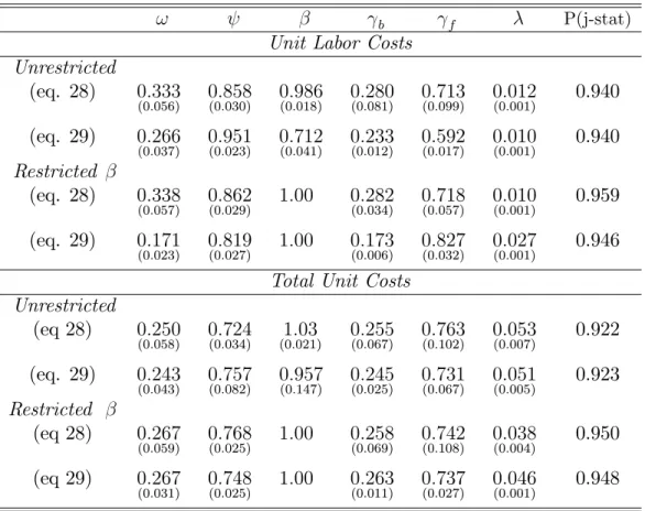
{Table 2: NKPC Estimates: Unit Labor Cost vs Total Unit Costs}
Table 2 gives non-linear instrumental variables, (GMM, IV) estimates of the deep structural parameters in equation (24) using labor unit costs and total unit costs as proxies for marginal cost, respectively. The instrument set used is four lags of the measure of real marginal costs, in‡ation, wage in‡ation and commodity price in‡ation.28 The results in Table 2, suggest that adding
non-labor unit costs to the familiar unit labor costs improves on the existing empirical support for (a) the role of real marginal cost as the driving variable in the NKPC and (b) the forward looking expectations-based new Keynesian Phillips curve.
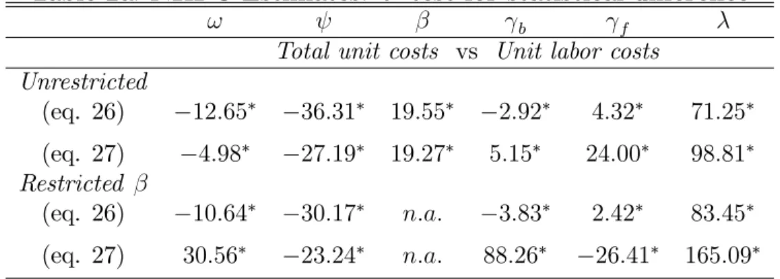
Focusing …rst on the real marginal cost coe¢ cient, , Table 2 shows that total unit costs imply a higher , than the traditional measure of real unit labor cost. Further, tstatistics for the di¤erence in these estimated coe¢ -cients, show that even when standard errors are taken into account the size of is signi…cantly di¤erent (higher in absolute terms) when total unit cost is used as the measure of marginal cost, irrespective of the orthogonality condition and restriction on beta.29
To further establish, independently of our structural model, whether the total unit costs NKPC is a better speci…cation than the unit labor costs
28Here we use the most parsimonious instrument set possible to avoid the estimation
bias that arise in small samples with too many over-identifying restrictions (see Staiger and Stock (1987). However, in Table 3, where we compare our marginal cost proxy to that used in Gali, Gertler and Lopez-Salido (2005) we use, for comparative purposes, exactly the same instruments as those employed by the latter study.
29Table 2a in the Appendix, reports the t-statistics for the di¤erence in the estimated
NKPC, we also conduct a non-nested test. The results are summarized in Table 3. Although the de…nition of total unit cost nests unit labor cost, equation (24) does not lend itself to the traditional F-tests for nested models, since it only includes one marginal cost variable. We therefore treat the unit labor cost NKPC and total unit labor cost NKPC as two di¤erent non-nested models focusing on the choice of regressors, that is total unit cost versus unit labor cost. In this regard we employ the Davidson and MacKinnon (1981) J-test which is based on the comprehensive approach and the Godfrey (1983) non-nested test for instrumental variable estimators.30
{Table 3: NKPC Estimates: Non-nested Tests}
Table 3, indicates that while we reject the null hypothesis for the labor unit cost NKPC model in favour of the total unit cost model, we cannot reject the null for the total unit cost NKPC model; hence total unit cost NKPC appears to be a better explanatory variable for in‡ation than the standard labor unit cost NKPC.
3.2.1 Total Unit Costs and Forward Looking Behavior
The results in Table 2 also suggest that when total unit costs are used as the driving variable in the NKPC, the coe¢ cients on the structural parame-ters indicating backward looking behavior, (i.e. !; and b) are generally lower, and those indicating forward looking behavior (i.e. f and ) are
generally higher, than their respective labor unit cost counterparts. To test the robustness of this result we perform a number of tests, including try-ing di¤erent sample periods, applytry-ing a time varytry-ing trend and also testtry-ing
the implications of total unit costs for fundamental in‡ation and in‡ation persistence.31
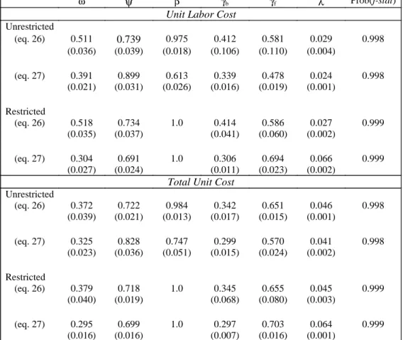
First, we test whether the relatively stronger forward looking behavior implied by total unit costs, holds in periods of high in‡ation volatility. Us-ing unit labor costs on US data, Zhang, Osborn and Kim (2008) …nd very little empirical support for the role of forward expectations-based in‡ation persistence in the high and volatile in‡ation period 1968:1 to 1981:4. When we estimate the NKPC structural parameters for the same sample period, we …nd that the coe¢ cient on unit labor costs is, = 0:024 (0:001) (stan-dard errors in brackets) with b = 0:339 (0:016) and f = 0:478 (0:020).32
However, for the same sample period the use of total unit costs produces,
= 0:0407 (0:0016), with b = 0:299 (0:015)and f = 0:570 (0:024).33 This,
consistently with Table 2, suggests thattotal unit costs indicate a larger role for forward looking behavior than that implied by unit labor costs. It also suggests, that much of the evidence supporting a backward NKPC might have been somewhat biased by the use of unit labor costs as a proxy for marginal cost.
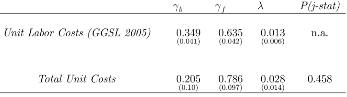
Similar results are presented in Table 4, where we examine the role oftotal unit costsusing the exact sample period and instruments used by Gali,Gertler and Salido-Lopez (2005) (GGSL 2005),
{Table 4: Comparative estimates of NKPC with GGSL 2005}
Total unit costs are again shown to produce a statistically signi…cant co-e¢ cient that is larger than that produced by unit labor costs. Note also
31The latter two tests are discussed in sections 3.2.1 and 3.3 respectively. 32For the full details see Table 6 in the Appendix.
33The di¤erence in the coe¢ cients on
f between these two marginal cost proxies is
that in relation to Table 2, that includes the more recent years of relatively high in‡ation stability (late 1980s to 2003), Table 4 suggests a larger role of expectations-based in‡ation persistence, f, when total unit costs are used instead of labor unit costs.
We also …nd that total unit costs imply a degree of price stickiness, , that is closer to the values supported by micro data. Speci…cally, the estimate from the …rst orthogonality condition implies an average price duration of 3.6 quarters, while the second orthogonality condition implies a duration of 4.1 quarters. Even after we account for the standard errors, these estimates are closer to the 3 to 4 quarters found by Blinder (1994) using micro data, than a duration of 5 quarters or higher which is typically found in the empirical NKPC literature.34
{Table 5: NKPC, GMM Estimates - detrended unit cost}
Consistently with the literature, the above estimations are based on devi-ations of unit labor costs and total unit cost from their respective sample mean. However, this may not be appropriate if there are changes in the mean over time, which as …gures 1, 2 and 3 suggest, is likely. In this regard, similar to Gwin and VanHoose (2007) we use the HP detrended measures of marginal cost along with the same instrument set. Table 5 indicates that the results do not change signi…cantly for total unit costs. We next check the implications of total unit costs for fundamental in‡ation and persistence.
34Note that Sbordone’s (2001) main baseline calibrated results (using labor unit costs)
show price contracts of 4.7 quarters. To obtain plausible estimates for price stickiness she had to assume (a) the share of capital was 0.25 , (b) the mark-up …rms charged was 20%. The latter assumption is signi…cantly higher than the 10% found in the literature see Gagnon and Khan (2004) and Basu and Fernald (1997). Also Gagnon and Khan’s (2004), (also using unit labor costs), estimates of beta (0.86 is the largest value reported) are very low with respect to near unity as suggested for the US in Gali and Gertler (1999).
3.2.2 Actual versus Fundamental In‡ation
To assess the explanatory power of the NKPC using total unit cost as opposed to unit labor costs, we estimate the model-consistent or ‘fundamental’(Gali and Gertler 1999) in‡ation rate and compare this with the actual in‡ation rate. As Gali and Gertler (1999) show, the hybrid NKPC has the following closed form, t = 1 t 1+ 2 f 1 X s=0 s 2 Etfmcct+sjztg where 1 = 1 p1 4 b f 2 f and 2 = 1+p1 4 b f
2 f are the small and large roots
of (24) respectively and zt is a subset of the market’s information set
con-taining current and lagged values of in‡ation and real marginal cost i.e. zt = f t; :::; t q+1;mcct; :::;mcct q+1g0. If we assume that the data
generat-ing process for zt can be represented by the following VAR(q), zt =Azt 1+
vt, where A is a 2q x 2q companion matrix, then as Campbell and Shiller
(1987) demonstrates the second term in the equation, (i.e. discounted future marginal cost) is,
2 f 1 X s=0 s 2 Etfmcct+sjztg= 2 f h0 2A(1 2A) 1zt
from which the fundamental in‡ation is,
f
t = 1 t 1+ 2 f
h0 2A(1 2A) 1zt
where h0 is a 1 x 2q selection row vector that extracts the forecast of real marginal cost (i.e. the …rst element of A(1 2A) 1zt). Accordingly, we
derive the present value of future marginal cost from a VAR(3) model.35 35The Schwarz and Hannan-Quinn information criteria suggest a lag length of 3 for the
The resulting fundamental in‡ation fortotal unit cost andunit labor cost
versus actual in‡ation are shown in …gures 4a and 4b. {Figure 4a} {Figure 4b}
These …gures show that the total unit cost driven NKPC matches actual in‡ation much better than its unit labor cost counterpart. 36
3.3
Total Unit Costs and In‡ation Persistence
In this section we examine how the in‡ation persistence implied by our total unit cost driven NKPC, that is based on the structural parameters of our model, compares to that implied by a VAR model using real data. Following Fuhrer (2006), we compute the theoretical autocorrelation function (ACF) for the NKPC using the coe¢ cients from Table 2 (as implied by the orthog-onality condition (27) for the unrestricted case ) and then compare it to the autocorrelation function from the simple three variable VAR in the in‡ation rate, federal funds rate and real marginal cost, estimated over the period 1966 to 2003.37 The ACF of the VAR gives an estimate of the persistence
that is consistent with the data and is independent of any structural or theo-retical restriction. Fuhrer (2006) suggests that the reduced-form persistence obtained from the VAR serves as a useful benchmark. By comparing this reduced-form persistence with that implied by the pure NKPC model we can
36Moreover, the generalized R2 of Pesaran and Smith (1994), which is an
asymptoti-cally valid model selection criterion and measure of …t for nested and non-nested models estimated with instrumental variables, are 0.899 for the total unit cost NKPC and 0.706 for unit labor cost NKPC.
37We are grateful to Je¤ Fuhrer for sharing his programs for generating the ACFs and
con…dence bands for the NKPC and VAR. For a detailed derivation of the ACF for in‡ation see Fuhrer (2006).
assess whether the persistence in in‡ation emanates from the driving variable or whether it is intrinsic.
Fuhrer (2006) shows that since the coe¢ cient on the real marginal cost (as implied by unit labor costs) is at most around 0.035, for the theoretical NKPC to lie within the 75% con…dence the coe¢ cient on the backward looking in‡ation needs to have a value of 0.6, which contradicts the suggested values in the Gali et al studies, (which is around 0.3).
However, when we use Fuhrer’s ACF graph with total unit costs as the marginal cost proxy, the theoretical NKPC lies well within the 70% con…-dence. In particular, using the coe¢ cient estimates in Table 2, …gure 5 shows the graph of the theoretical ACF implied by the total unit cost driven NKPC, (TUC NKPC - solid line). This …gure also shows the ACF graph as implied by the unit labor cost driven NKPC, (Fuhrer (2006) - dashed line), as well as the ACF and the corresponding con…dence interval implied by the VAR (VAR –dotted line).38
{Figure 5}
In contrast to the ACF derived from the unit labor cost model (Fuhrer 2006), the ACF derived from the total unit cost driven NKPC is much closer to the benchmark VAR ACF, and although at points is slightly higher, it is still within the 70% con…dence band corresponding to Fuhrer (2006). In general, thetotal unit cost driven NKPC generates persistence that matches the data reasonably well. This also means that a lower b is now required to
capture the observed persistence in in‡ation, as a larger part of in‡ation is now captured by the real marginal cost proxy. In particular, the estimated value of b = 0:245, that we use to derive the theoretical ACF in Figure 5, is much lower than the value of b = 0:6that Fuhrer (2006) found was required
for the NKPC to su¢ ciently capture the persistence in in‡ation under unit labor costs.
4
Concluding Remarks
Wolman (1999), suggests that in assessing the new Keynesian Phillips curve more re…ned estimates of marginal cost than the labor income share should be investigated. Extending the data already used in the literature, by using both labor and non-labor payments in nonfarm GDP so as to match our theory-based marginal cost, we construct atotal unit cost that we use as our real marginal cost proxy in the new Keynesian Phillips curve.
It is shown that adding non-labor unit costs to the familiar labor unit costs, (i) improves on the …t of observed in‡ation and hence on the exist-ing empirical support for real marginal costs as the drivexist-ing variable in the NKPC; (ii) imply a duration of …xed nominal contracts that is much closer to those suggested by …rm-level surveys, than that implied by merely labor unit costs; (iii) total unit costs suggest a larger role for forward looking behavior and expectations-based in‡ation persistence than that implied by the con-ventional unit labor costs. This e¤ect is shown to hold even in the relatively high and volatile in‡ation periods of the 1970’s where the use of unit labor costs suggest a very weak forward looking behavior. Intuitively, this might be because in periods of increased uncertainty and high in‡ation volatility, expectations about future in‡ation may be more relevant to …rms’decisions about non-labor costs, such as on borrowing costs and investment in new capital.
Wolman’s suggestion to investigate more re…ned estimates of marginal cost is recently attracting more attention. We believe that richer data of
marginal cost proxies, particularly from data that also re‡ect information about key leading economic indicators, such as expectations about interest rates, borrowing costs and investment, that are so far largely neglected in empirical estimations of the NKPC, may substantially improve the existing empirical evidence on forward looking behavior in price setting and in‡ation.
References
Adolfson, M., Laséen, S., Lindé, J., Villani, M., 2005. The role of sticky prices in an open economy DSGE model: a Bayesian investigation. Journal of the European Economic Association Papers and Proceedings, 3 (2–3), 444–457. Agénor, P.R., Bratsiotis, G.J., Pfajfar, D., 2011. Monetary Shocks and the
Cyclical Behavior of Loan Spreads. Centre for Growth and Business Cycle Research Discussion Paper Series, University of Manchester, No. 156. Atta-Mensah, J., Dib, A., 2008. Bank lending, credit shocks, and the
transmis-sion of Canadian monetary policy. International Review of Economics and Finance, 17, 159–176
Basu, S., and J.G. Fernald., 1997. Returns to Scale in U.S. Production: Esti-mates and Implications. Journal of Political Economy, 105 (2), 249-83. Bils, M., Klenow, P., 2004. Some evidence on the importance of sticky prices.
Journal of Political Economy 112, 947–985.
Blinder, A., Canetti, E., Lebow, D., Rudd, J., 1998. Asking about Prices: A New Approach to Understand Price Stickiness. Russell Sage Foundation, New York.
Bjørnland, H. C., Leitemo K., Maih J., 2009. Estimating the Natural Rates in a simple New Keynesian Framework. Norges Bank working paper 2007/10. Campbel, Y. J., Shiller R., 1987. Cointegration Tests of Present Value Models.
Journal of Political Economy, vol. 95, no. 5, 1062–1088.
Cantore C., Levine P., Yang B., 2010. CES Technology and Business Cycle Fluctuations. Working Paper, University of Surrey.
Chadha, J.S., Nolan. C., 2004. Output, In‡ation and the New Keynesian Phillips Curve. International Review of Applied Economics, 18, 3, 271-287. Chevalier, J., Kashyap, A., Rossi, P., 2003. Why Don’t Prices Rise During
Pe-riods of Peak Demand? Evidence from Scanner Data". American Economic Review 93, 15–37.
Chowdhury, I., Ho¤mann, M., and Schabert, A., 2006. In‡ation Dynamics and the Cost Channel of Monetary Transmission. European Economic Review, 50, 995-1016.
Christiano L.J., Eichenbaum M., Evans C., 2001. Nominal rigidities and the dynamic e¤ects of a shock to monetary policy. Proceedings, Federal Reserve Bank of San Francisco (June).
Coenen, G., Levin, A.T., Kai, C., 2007. Identifying the in‡uences of nominal and real rigidities in aggregate price-setting behavior. Journal of Monetary Economics, 54(8), 2439-2466.
Cook, D. 1999. The Liquidity E¤ect and Money Demand. Journal of Monetary Economics, 43, 377–90.
Davidson, R., MacKinnon J., 1981. Several Tests for Model Speci…cation in the Presence of Alternative Hypotheses. Econometrica Vol. 49, No. 3, 781-793. De Walque, G., Smets, F., Wouters R., 2004. Price Setting in General
Equilib-rium: Alternative Speci…cations. Mimeo, National Bank of Belgium.
Di Bartolomeo, G., Manzo, M. 2007. Do tax distortions lead to more indeter-minacy? A New Keynesian perspective. MPRA Working Paper No. 3549, (November).
Faia, E., Monacelli, T., 2007. Optimal Interest Rate Rules, Asset Prices, and Credit Frictions. Journal of Economic Dynamics and Control, 31, 3228-54. Fuhrer, J., 2006. Intrinsic and Inherited In‡ation Persistence. International
Jour-nal of Central Banking, 3, 2, 49-86.
Gagnon, E., Khan H. 2005. New Phillips Curve Under Alternative Production Technologies for Canada, the United States and the Euro Area. European Economic Review, 49, 1571 –1602.
Gali, J., Gertler M., 1999. In‡ation Dynamics: A Structural Econometric Analy-sis. Journal of Monetary Economics, 44, 2, 195-258.
Gali, J., Gertler M., Lopez-Salido, J.D., 2001. European In‡ation Dynamics. European Economic Review, 45, 1237-1270
Gali, J., Gertler M., Lopez-Salido, J.D., 2005. Robustness of the Estimates of the Hybrid New Keynesian Phillips Curve. Journal of Monetary Economics, 52, 2, 1107-1118.
Gali, J., Gertler M. Lopez-Salido, J.D. 2007, Markups, gaps and the welfare costs of business zuctuations. The Review of Economics and Statistics, 89: 44-59.
Godfrey, L.G., 1983. Testing Non-Nested Models After Estimation by Instru-mental Variables or Least Squares. Econometrica, 51, 2, 355-365.
Goodfriend, M., McCallum, B.T., 2007. Banking and Interest Rates in Mone-tary Policy Analysis: A Quantitative Exploration. Journal of MoneMone-tary Eco-nomics, 54, 1480-507.
Gwin, C.R., VanHoose, D.D., 2007. Disaggregate Evidence On Price Stickiness And Implications For Macro Models. Economic Inquiry, Western Economic Association International, 46, 4, 561-575.
Gwin, C.R., VanHoose, D.D., 2008. Alternative measures of marginal cost and in‡ation in estimations of new Keynesian in‡ation dynamics. Journal of Macroeconomics, Elsevier, 30, 3, 928-940.
Hall, S., Walsh, M., Yates, T., 2000. Are UK Companies’prices sticky? Oxford Economic Papers 52, 425–446.
Hnatkovska, V., Lahiri, A., Vegh, C.A., 2008. Interest Rates and the Exchange Rate: A Non-Monotonic Tale. NBER Working Paper No. W13925.
Lawless, M., Whelan, K., 2007. Understanding the Dynamics of Labour Shares and In‡ation. European Central Bank Working Papers Series, no. 784. Lindé, J. 2005 Estimating New Keynesian Phillips Curve: A Full Information
Maximum Likelihood Approach. Journal of Monetary Economics, 52, 6, 1135-1149.
Matheron, J.,Maury, T., 2004. Supply-Side Re…nements and the New Keynesian Phillips Curve. Economic Letters, 82, 391-396.
Neiss, K.S., Nelson, E. 2005. In‡ation Dynamics, Marginal Cost, and the Out-put Gap: Evidence from Three Countries. Journal of Money, Credit, and Banking, 37, 6, 1019-1045.
Neiss, K.S., Pappa E., 2005. “Persistence Without Too Much Price Stickiness: The Role of Factor Utilisation”, Review of Economic Dynamics 8, 1231-1255. Pesaran, M.H., 1974. On the General Problem of Model Selection. Review of
Economic Studies, 41, 153-171.
Pesaran, M.H., Deaton A., 1978. Testing Non-Nested Nonlinear Regression Mod-els. Econometrica, 46, 3, 677-694.
Pesaran, M.H., Smith, R., 1994. A Generalized R2 Criterion for Regression Models Estimated by the Instrumental Variables Method. Econometrica, 62, 3, 705-710.
Ravenna, F., Walsh, C.E., 2006. Optimal Monetary Policy with the Cost Chan-nel. Journal of Monetary Economics, 53, 199-216.
Rotemberg, J., 1982. Monopolistic Price Adjustment and Aggregate Output. Review of Economic Studies, 49, 517-31.
Rotemberg, J., Woodford M., 1999. The Cyclical Behaviour of Prices and Costs. NBER Working Paper 6909
Rotemberg, J., Woodford M., 1997. An Optimization-Based Econometric Frame-work for the Evaluation of Monetary Policy. NBER Technical Working Paper T233.
Rudd J., Whelan, K., 2007. Modelling In‡ation Dynamics a Critical Review of the Research. Journal of Money Credit and Banking, vol. 39, pg. 155-170. Rudd J., Whelan, K., 2005. New tests of the new-Keynesian Phillips curve.
Journal of Monetary Economics, vol. 52(6), pages 1167-1181,
Rudd J., Whelan, K., 2002. “Does Labour Income Share Drive In‡ation,” Fi-nance and Economics Discussion Series, no. 30.
Sbordone, A., 2005. Do Expected Future Marginal Cost Drive In‡ation Dynam-ics. Journal of Monetary Economics, vol. 52, no.6, pg. 1183-1197.
Sbordone, A., 2002. Prices and Unit Labor Costs: A New Test of Price Sticki-ness, Journal of Monetary Economics, 49, 2, 265-292.
Staiger, J., Stock, J., 1987. Instrumental variables regression with weak instru-ments. Econometrica 65, 3, 557–586.
Wolman, A., 1999. Sticky prices, marginal cost, and the behavior of in‡ation. Federal Reserve Bank of Richmond Economic Quarterly, 85, 29–48.
Woodford, M., 2001. Firm-Speci…c Capital and the New Keynesian Phillips Curve. International Journal of Central Banking, vol. 1, No.2, pg. 2-46. Zhang C., Osborn D. R., Kim, D.H., 2008. The New Keynesian Phillips Curve:
From Sticky In‡ation to Sticky Prices. Journal of Money, Credit and Bank-ing, 40, 4, 667-699.
Data De…nitions
All the data, with the exception of commodity price index, are sourced from the U.S. Department of Commerce Bureau of Economic Analysis and the US Bureau of Labor Statistics. The commodity price index is the spot commodity index sourced from the Commodity Research Bureau at: http://www.crbtrader.com/crbindex/
Labor Cost (nonfarm): Source: US Bureau of Labor Statistics
Non-Labor Costs (nonfarm)= Non-Labor Payment (non farm) - Corporate Pro…ts (nonfarm)
Non-Labor Payments (nonfarm): Source: US Bureau of Labor Statistics. These payments include pro…ts, consumption of …xed capital, taxes on production and imports less subsidies, net interest and miscellaneous payments, business current transfer payments, rental income of persons, and the current surplus of government enterprises.
Corporate Pro…ts (nonfarm):US Bureau of Economic Analysis, Table 6.16D (sum of pro…ts of all non-farm domestic industries)
In‡ation - Change in the log of the GDP de‡ator.
Nominal (nonfarm) GDP: US Bureau of Economic Analysis, Table 1.3.5
Output Gap: Log di¤erence between real GDP and the Hodrick-Prescott …ltered trend.
Total Costs (nonfarm) = Labor Cost (nonfarm) + Non-Labor Costs (non-farm)
Unit Labor Costs (nonfarm)= (log)Labor Cost (nonfarm) - (log)Nominal (nonfarm) GDP
Total Unit Costs (nonfarm)= (log)Total Costs (nonfarm) - (log)Nominal (nonfarm) GDP
Table 1: Break Point Tests in the Persistence of Marginal Cost Break Point Autocorrelation Coe¢ cient
Unit Labor Costs
1981:04 0.8262*
1990:01 0.8082*
1997:02 0.7627*
Non-Labor Unit Costs
1980:03 0.8568*
2000:02 0.7947*
Total Unit Costs
1978:03 0.9008*
1997:02 0.8579*
2000:01 0.6774*
Note: This table presents results of tests for shifts in persistence using the Perron and Vo-gelsang (1992) innovational outlier model over the period: 1966Q1 to 2003Q4. * indicates signi…cance at the 5% level.
Table 2: NKPC Estimates: Unit Labor Cost vs Total Unit Costs
! b f P(j-stat)
Unit Labor Costs Unrestricted (eq. 28) 0:333 (0:056) 0:858 (0:030) 0:986 (0:018) 0:280 (0:081) 0:713 (0:099) 0:012 (0:001) 0.940 (eq. 29) 0:266 (0:037) 0:951 (0:023) 0:712 (0:041) 0:233 (0:012) 0:592 (0:017) 0:010 (0:001) 0.940 Restricted (eq. 28) 0:338 (0:057) 0(0::862029) 1:00 (00::282034) 0(0::718057) 0(0::010001) 0.959 (eq. 29) 0:171 (0:023) 0(0::819027) 1:00 (00::173006) 0(0::827032) 0(0::027001) 0.946
Total Unit Costs Unrestricted (eq 28) 0:250 (0:058) 0(0::724034) (01::021)03 0(0::255067) 0(0::763102) 0(0::053007) 0.922 (eq. 29) 0:243 (0:043) 0(0::757082) (00::957147) 0(0::245025) 0(0::731067) 0(0::051005) 0.923 Restricted (eq 28) 0:267 (0:059) 0(0::768025) 1:00 (00::258069) 0(0::742108) 0(0::038004) 0.950 (eq 29) 0:267 (0:031) 0(0::748025) 1:00 (00::263011) 0(0::737027) 0(0::046001) 0.948
Note: This table reports non-linear IV (GMM) estimates of the deep structural parame-ters in equation (24), using labor unit cost and total unit costs as proxies to marginal cost. The estimation uses quarterly data over the period: 1966:Q1-2003:Q4. The instru-ment set includes four lags of the real marginal cost proxy, in‡ation, wage in‡ation and commodity price in‡ation. Standard errors are shown in brackets. A 12-lag Newey-West estimate of the covariance matrix is used. The last column presents the Hansen’s J-test for overidentifying restrictions.
Table 3: NKPC Estimates: Non-nested Tests
b f J-Test Godfrey
Unit Labor Costs 0:280
(0:035) 0(0::713037) (00::012006) 2:72 3:44
Total Unit Costs 0:255
(0:045) 0(0::763046) (00::053015) 0:17 0:11
Note: This table reports the GMM estimates of the reduced-form of equation (24), using quarterly data over the period 1966 Q1 to 2003 Q4. The instrument set includes four lags of the measure of real marginal costs, detrended output, wage in‡ation and in‡ation. Standard errors are given in parenthesis below. A 12-lag Newey-West estimate of the covariance matrix is used. The last two columns give the Davidson –McKinnon J-test and Godfrey non-nested tests. Asterisks (*) denote signi…cance at the 5% level.
Table 4: Comparative estimates of NKPC with GGSL (2005)
b f P(j-stat)
Unit Labor Costs (GGSL 2005) 0:349
(0:041) 0(0::635042) 0(0::013006) n.a.
Total Unit Costs 0:205
(0:10)
0:786
(0:097)
0:028
(0:014) 0.458
Note: This table reports GMM estimates of equation (24), using quarterly data over the period 1960 Q1 to 1997 Q4. As in Gali, Gertler and Lopez-Salido (2005) the instrument set includes two lags of the real marginal costs proxy, in‡ation, detrended output, and wage in‡ation and four lags of in‡ation. The upper panel reports the comparative results from the baseline estimates in Gali, Gertler and Lopez-Salido (2005). Standard errors are given in parenthesis below. A 12-lag Newey-West estimate of the covariance matrix is used. The last column presents the Hansen’s J-test for overidentifying restrictions.
Table 5: NKPC, GMM Estimates - detrended unit cost
t= b t 1+ fEt t+1+ mct
b f Prob(j-stat)
Unit Labor Costs 0:288
(0:035) 0(0::706037) (00::036012) 0:954
Total Unit Costs 0:266
(0:039) 0(0::729040) (00::047016) 0:939
Note: This table reports the GMM estimates of equation (24), using the Hodrick-Prescott …ltered detrended measures of marginal cost. The estimation uses quarterly data over the period 1966:Q1 to 2003:Q4. The instrument set includes four lags of the measure of real marginal costs, in‡ation, wage in‡ation and commodity price in‡ation. Standard errors are given in parenthesis below. A 12-lag Newey-West estimate of the covariance matrix is used. The last column presents the Hansen’s J-test for overidentifying restrictions.
APPENDIX
(Not for Publishing)
Appendix A: Further empirical tests
Table 2a,gives the t-statistics for the di¤erence in the estimated parameters in Table 2 using the standard test for di¤erence in means. The null hypothesis is that there is no signi…cant di¤erence in the estimates. The critical value of the t-statistics at the 5 percent level with 302 degrees of freedom is 1.98 and as such we reject the null hypothesis in all cases for all coe¢ cients. Therefore, we conclude that, even when the standard errors are taken into account, the size of lambda is signi…cantly di¤erent (higher in absolute terms) when total unit cost is used as the measure of marginal cost, irrespective of the orthogonality condition and restriction on beta.
Table 2a: NKPC Estimates: t- test for statistical di¤erence
! b f
Total unit costs vs Unit labor costs Unrestricted (eq. 26) 12:65 36:31 19:55 2:92 4:32 71:25 (eq. 27) 4:98 27:19 19:27 5:15 24:00 98:81 Restricted (eq. 26) 10:64 30:17 n:a: 3:83 2:42 83:45 (eq. 27) 30:56 23:24 n:a: 88:26 26:41 165:09
Note: This table reports the t-statistic for di¤erences in coe¢ cients of the NKPC estimates using total unit cost and unit labor cost. The test is a two-tailed test with the null hypothesis,H0 :xT U C xU LC = 0, against the alternativeH0 :xT U C 6=xU LC. The
test statistic is t = (xT U C xU LC)=psp, where sp = 2(s2T U C +s2U LC)=v and the
degrees of freedom are v = 2n 2 = 302; s is the standard error of the coe¢ cient estimate. Stars (*) denotes the signi…cance at the 5% level.
Test for the Non-Nested Model
We are interested in comparing two competing models: Mx : t =XtA+ut
Mz : t =ZtB+et,
where t is the in‡ation rate, Xt = ( t 1; E t+1;total unit costs)
0
and Zt =
( t 1; E t+1;unit labor costs)
0
; utand et are random errors andA and B are
the matrix of coe¢ cients estimated using GMM (instrumental variables). De-…neW as the matrix of instruments andQ(W)the projectionW(W0W) 1W0. The null hypothesis is that Mi, i=x; z is the valid model against the
alter-native Mj, j = x; z (i 6= j). The augmented model is t = (1 ')XtA+
'ZtB +"t. The null hypothesis tested is ' = 0. Yet, since ' cannot be
separately estimated in this model we use the Davidson and MacKinnon’s (1981) test.
For the Godfrey non-nested test for instrumental variables estimators, the augmented model is,
t =XtA+ (XetAe) +"t,
where Ae is the IV estimate of A; Xet is the matrix of OLS residuals of the
regression of Xbt onZbt; where Xbt =Q(W) X is the …tted values of the OLS
regression of X on W and Zbt = Q(W) Z is the …tted values of the OLS
regression ofZ onW. The test for the validity ofMx is therefore a standard
Table 6, provides the empirical estimates for the high and volatile in‡ation period sample used in Zhang, Osborn and Kim (2008). In the text we only report the key coe¢ cients as shown by (eq 27), for the unrestricted case.
Table 6: NKPC Estimates: Unit Labor Cost vs Total Unit Cost (1968Q1-1981Q4)
Note: This table reports non-linear IV estimates (GMM) of the deep structural parameters in equation (25), using labor unit cost and total unit costs as proxies for marginal cost. The estimation uses quarterly data over the period: 1968:Q1-1981:Q4. The instrument set includes four lags of the real marginal cost proxy, inflation, wage inflation and commodity price inflation. Standard errors are shown in brackets. A 12-lag Newey-West estimate of the covariance matrix is used. The last column presents the Hansen’s J-test for overidentifying restrictions.
ω ψ β γb γf λ Prob(j-stat)
Unit Labor Cost Unrestricted (eq. 26) 0.511 0.739 0.975 0.412 0.581 0.029 0.998 (0.036) (0.039) (0.018) (0.106) (0.110) (0.004) (eq. 27) 0.391 0.899 0.613 0.339 0.478 0.024 0.998 (0.021) (0.031) (0.026) (0.016) (0.019) (0.001) Restricted (eq. 26) 0.518 0.734 1.0 0.414 0.586 0.027 0.999 (0.035) (0.037) (0.041) (0.060) (0.002) (eq. 27) 0.304 0.691 1.0 0.306 0.694 0.066 0.999 (0.027) (0.024) (0.011) (0.023) (0.002)
Total Unit Cost Unrestricted (eq. 26) 0.372 0.722 0.984 0.342 0.651 0.046 0.998 (0.039) (0.021) (0.013) (0.017) (0.015) (0.001) (eq. 27) 0.325 0.828 0.747 0.299 0.570 0.041 0.998 (0.023) (0.036) (0.051) (0.015) (0.024) (0.002) Restricted (eq. 26) 0.379 0.718 1.0 0.345 0.655 0.045 0.999 (0.040) (0.019) (0.068) (0.080) (0.003) (eq. 27) 0.295 0.699 1.0 0.297 0.703 0.064 0.999 (0.016) (0.016) (0.007) (0.016) (0.001)