On Comparison of Some Imputation Techniques in Multivariate
Data Analysis
Chukwu, A. U1., Ezichi, O. N2.& Dike A. O3* 1&2
Department of Statistics, University of Ibadan, Ibadan, Nigeria. 3
Department of Maths/Statistics, Akanu Ibiam Federal Polytechnic, Unwana,Nigeria. *[email protected]
Abstract
Listwise or pairwise deletion as the method of handling missing data in multivariate data leads to loss of statistical power, biased results and underestimation of standard errors and P-values.Four imputation techniques namely Regression, Stochastic, Expectation-Maximization (EM) and Multiple Imputation (MI) were considered and compared in terms of preserving the original distribution of the (multivariate) data and the relationships among the variables before the techniques were applied. Results show that none of the techniques performed absolutely better than the rest leaving the choice of imputation techniques in any dataset on the objectives of the researcher.
Keyword: Imputation, missing data, Expectation Maximization, Multiple Imputation, Root Mean Square Error.
1.0 Introduction
Method of handling missing data in some statistical software like SAS, S-Plus and SPSS is listwise deletion. This involves dropping any case with missing value. Consequently, statistical power is lost, biased results are obtained and underestimation of standard errors and P-values are usually observed.
Alternatively, imputation can be applied which according toEveritt (2002) is a process of estimating missing values using the non-missing information available for the subject. It addresses the problem of reduction in statistical power. There are several imputation techniques which include mean imputation (the average value is filled in), regression imputation (a regression model is used to predict the missing value), hot deck imputation (which imputes new values from similar cases), Stochastic imputation and the more recent methods like Maximum Likelihood, Multiple Imputation, Expectation Maximization (EM), etc. However, only four techniques are considered in this work namely: Regression imputation, Stochastic imputation, Expectation-Maximization and the Multiple Imputation. Von Hippel (2007) suggested that several factors should be considered before a technique is chosen. Such factors include type of parameter estimates that should be generated (biased or unbiased), non-response rate, nature of the missing data and availability of an auxiliary data that are correlated with characteristic of interest.
1.1 Non-Response Rate
For non-response rate, the researcher should consider percentage of missing data for each of the variable. ‘Small’ percentage of missing value is less problematic and may be corrected by simpler imputation techniques like overall mean or class-mean imputation technique where applicable. There’s no consistent definition of ‘small amount of missing data’. However, for Little and Rubin (2002) it ranges from 5% or less of values.
1.2 Nature of Missing Data
The researcher needs to establish whether data are missing completely at random (MCAR), missing at random (MAR) or missing not at random (MNAR). This factor determines the choice of the technique to choose as well as the case deletion method to adopt. If data are MCAR then listwise deletion yield unbiased results but if the data are not MCAR, listwise deletion will introduce bias because the sub-sample of case represented by the missing data are not representative of the original sample (and if the original sample was itself a representative sample of a population, then the complete cases are not representative of that population either. Brick and Kalton (2000)
1.2.1Missing Completely at Random (MCAR)
Here, the probability of response to a variable of interest, Y, is the same for all the units in the population. This means that the probability of response does not depend on the auxiliary variable(s), or the variable of interest, Y.Roughly speaking, the tendency for a data point to be missing is completely random. Pickles (2005) points out that for MCAR, the probability of missingness is a constant. This implies that Pi = P(i ϵ Sr) = P. ∀ i ∊ U. Where Sr is Sample of respondents for a given item and U is the target population of size N. Formally, when data are MCAR, evidently the set of objects with no missing data is also a random sample from the source population. Hence, most techniques for handling missing data under MCAR including listwise deletion yield unbiased results. According to Fellegi and Holt (1976), the imputed estimator, Ӯ* for the population mean will be unbiased if data are MCAR. A statistical test for MCAR is a Chi-square test which is provided in the SPSS Missing Values Analysis (MVA) option. A significant value indicates that data are not MCAR.
1.2.2Missing at Random (MAR)
In this case, the probability of response to a variable of interest, Y is related to auxiliary variable(s) X. This implies that Pi = P(i ϵ Sr) = P(Xi). i.e. data are MAR if the probability of response to Y is not a function of its own value but a function of the values of the auxiliary variable(s). Generally, when data are MAR, a complete case analysis is no longer based on random sample from the source population. Hence, all simple techniques including the listwise deletion and overall mean imputations yield biasedresults. However, more advanced techniques like Stochastic Regression and Multiple Imputation techniques give unbiased results even when missing data are MAR.
The MAR test is a ‘‘Separate variance t-tests’’ which is also available on the SPSS Missing Values Analysis (MVA). A significant value indicates that data are MAR.
1.2.3Missing Not at Random (MNAR)
Often times, data are MNAR, implying that missingness is related to one or more of the outcome variables or that the missingness has a systematic pattern, Schaefer and Graham (2002). If there is a pattern to the missing values, the best decision is that they are MNAR. There are some simple ways researchers can examine their data to determine whether missing data follow a pattern. For instance, during instrument development like questionnaire, etc., response sets should include ‘don’t know’, ‘does not apply’ or ‘refused’ responses. These responses allow the researcher to distinguish among these ‘no answer’ responses. For example, if the majority of responses to an item asking for particular information which may be income, age, marital status, etc. are ‘refused’, the researcher will be confident that there is
a pattern to the responses. When missing data are MNAR, valuable information is lost from the data and there is no universal way of handling the missing data properly.
Although, data imputation techniques typically assume that at a minimum, data are MAR, more advanced imputation techniques are robust and produce nearly as good results without strictly meeting this assumption. Little and Rubin (2002).
2.0 Methodology
Procedures for data imputation using regression, stochastic, Expectation-Maximization (EM) and Multiple Imputation (MI) were described. The descriptive statistics, the statistical relationships and the normal Q-Q plots of the four variables were obtained and examined before and after imputation. The SPSS and R were used for the analysis.
2.1 Regression Imputation
This assumes a linear relationship between the variables used in the regression equation when there may not be one. We used the variable with the missing data as the dependent variable. Cases with the complete data for the predictor variables were used to generate the regression equation. Predictors of the missing values were identified using a correlation matrix. The best predictors were the variables with the highest correlations and were therefore used as the independent variables in a regression equation to predict missing values for the incomplete cases. That is for a variable Yi with missing values, a model
𝑌𝑖 = 𝛽0+ 𝛽1𝑌1 + 𝛽2𝑌2 + ⋯ + 𝛽(𝑖−1)𝑌(𝑖−1) 1.1
is fitted for the non-missing observations.
Where𝛽0,𝛽1, … , 𝛽(𝑖−1) are the estimated parameters of the model and𝑌1 , 𝑌2 , …,𝑌(𝑖−1)are the covariates used as predictors of the missing value. Multicollinearity was also considered.
2.2 Stochastic Imputation
We introduced an error term to Equation 1.1 because regression imputation doesn’t supply ‘uncertainty’ about the predicted value. Consequently, imputed data in 1.1 do not have an error term included in their estimation, thus the estimates fit perfectly along the regression line without any residual variance. This causes relationships to be over identified and underestimation of variance.
From the regression model in 1.1 above, the parameter estimates and the associated Variance-Covariance matrix of the fitted model are given by
𝛽0,∗ 𝛽1∗, … , 𝛽(𝑖−1)∗ and 𝜎2𝑄𝑖respectively. Where 𝑄𝑖 is the usual XIX matrix from the intercept and the variables 𝑌1 , 𝑌2 ,…,𝑌(𝑖−1). For each imputation, new parametersβ₀*, β₁*,…, β(i-1)* and σ2i* are drawn from the posterior predictive distribution of the missing data. Then a new model for the estimation of missing data is given by
𝑌𝑖 = 𝛽0+ 𝛽1𝑌1 + 𝛽2𝑌2 + ⋯ + 𝛽(𝑖−1)𝑌(𝑖−1)+ 𝑟𝑚𝑠𝑒 ∗ 𝜀𝑖 1.2 Where𝜀𝑖~ N (0,1) , and rmse is the Root Mean Square Error.
Clearly from 1.2, the error term for each model is a function of its Root Mean Square Error (rmse)
The procedure used here is summarized as follows:
(i) Regress the variable with the missing data on other variables. (ii) Obtain the root mean square error (Standard Error) of the estimate.
(iii) Compute the predicted value of the missing data given the values of other variables in the equation.
(iv) Add random variability (which is simply a product of the rmse and ϵi) to the predicted value Yi
2.3 Expectation–Maximization (EM) Imputation
The EM technique is a maximum likelihood based approach that works with the relationship between the unknown parameters of the data model and the missing data. We assumed a multivariate normal model. The procedure here is summarized as follows:
We first estimate the model parameters, then estimate the missing values, then use the filled-in dataset to re-estimate the parameters, then use the re-estimated parameters to estimate missing values, and so on. When the process finally converges on stable estimates the iterative process ends. Schaefer and Olsen (1998)
Recall that regression imputation underestimates the true variability in the data because there is no error associated with the imputed observations. Howell, D.C. (2008) points out that EM like Stochastic imputation corrects that problem by estimating variances and covariances that incorporate the residual variance from the regression. For instance, assume that we impute values for missing data on Y1from data on Y2, Y3and Y4, to find the estimated mean of Y1we
simply take the mean of that variable. Now that we have a new set of parameterestimates, we repeat the imputation process to produce another set of data. From that new set we re-estimate our parameters as above, and then impute yet another set of data. We continue this process in an iterative fashion until the estimates converge.
2.4 Multiple Imputation. MI uses a stochastic linear model.
𝑌𝑖 = 𝛽0+ 𝛽1𝑌1 + 𝛽2𝑌2 + ⋯ + 𝛽(𝑖−1)𝑌(𝑖−1)+ 𝜀𝑖 1.3 Where𝜀𝑖~ N(0,1) and 𝛽0,𝛽1, … , 𝛽(𝑖−1)are the parameters of the model.
From the term ‘multiple’, clearly we are required to impute several times. This implies that we shall have multiple complete dataset before we proceed with analysis. We then combine the results of those analyses and make inference. The process involves three different stages namely:
(i) Impute for the missing data k times using the above model.
(ii) The k completed datasets are analysed for the parameter estimates of interest. (iii) The results from the k completed datasets are combined for inference.
Step (iii) is broken down as follows:
Suppose k imputations were done, from each analysis, we calculate and save the estimates. The overall estimate is the mean of the individual estimates.
For the overall standard error for each variable, the within-imputation variance was first
𝑦 =𝑘1∑𝑘𝑖=1𝑊I 1.4 Wi i = 1,…,k are the variances for each dataset.
The between-imputation variance which is the variance of the variances of the variable in the
k dataset is given below as:
𝐵 =𝑘−11 ∑𝑘−1𝑖=1(𝑊𝑖 − 𝑦̅)2 1.5
The total variance is given by
T= 𝑦̅ + (1+ 1𝑛)B 1.6
Where (1 + 1
𝑛) is a correction factor. Then the overall standard error is the square root of T, (T)1/2
3.0 Example/ Analysis
We illustrate with a multivariate data of four variables obtained from the Records department of Bishop Shananhan Hospital, Nsukka, Enugu State, Nigeria. The variables are Age of the patients,(Y1,), Number of days they spent in the hospital (Y2), Blood pressure (Systolic)Y3 and their Weight (Y4). It is on 40 patients, with each patient providing information on each variable. There are 20 missing observations out of 160 across the data implying a non-response rate of 12.5%. Little’s Chi-Square test for MCAR and the ‘Separate Variance t-test’ for MAR were used to determine the nature of the missing data. Using the MVA(Missing Value Analysis) option on SPSS, under EM estimation, the Little’s MCAR test has the following values: Chi-Square = 14.006, degree of freedom = 14 and P-value = 0.449. At 5% level of significance, the null hypothesis that data are MCAR was accepted which implies that the probability of missingness is a constant and the set of items with no missing data is a random sample from the source population. Conclusion: Data are MCAR (5% level of significance).
Like in all practical cases and for a valid inference, the assumption of linear dependency amongst the variables was not taken for granted. We obtained a correlation matrix and tested for linear dependency among the variables. The essence of this was to determine how the four variables are correlated amongst themselves and subsequently determine the independent variable(s) that should be used in the imputation model for each variable. Using
𝐻0: 𝜌𝑖𝑗 = 0𝑉𝑠 𝐻1: 𝜌𝑖𝑗 ≠ 0 i ≠ j ∀𝑖𝑖 =1,2,3,4: ∀𝑗, 𝑗 = 1, 2,3,4 where 𝜌𝑖𝑗 signifies correlation between 𝑌𝑖 and 𝑌𝑗.
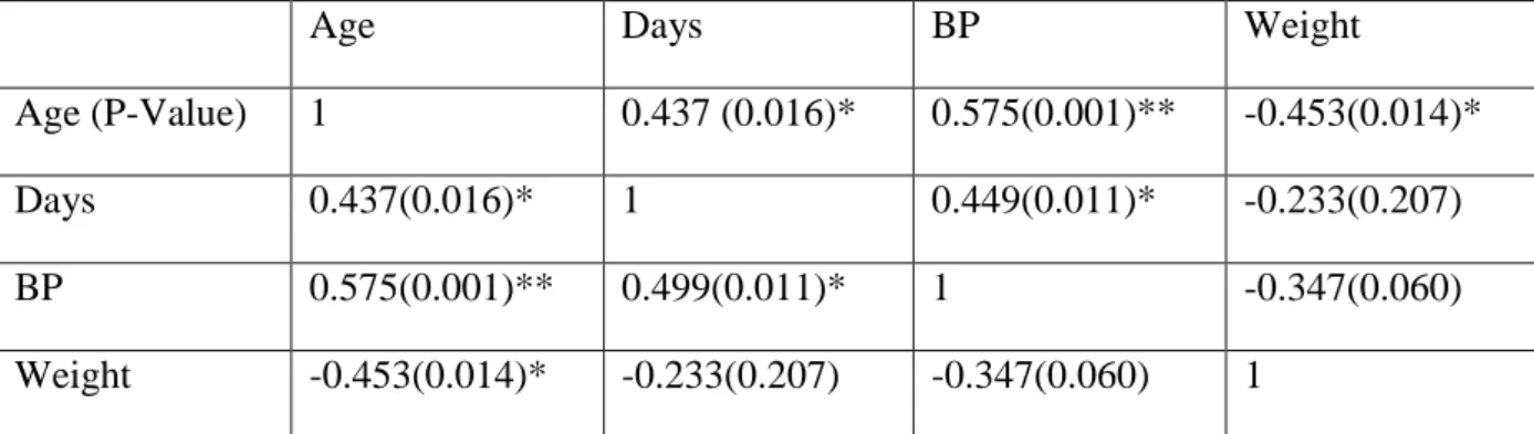
In Table 1 below, the values outside the bracket are the Pearson correlation coefficient while the values in the bracket are the P-values for the tests of hypothesis above.
Table 1. Correlation before imputation
Age Days BP Weight
Age (P-Value) 1 0.437 (0.016)* 0.575(0.001)** -0.453(0.014)*
Days 0.437(0.016)* 1 0.449(0.011)* -0.233(0.207)
BP 0.575(0.001)** 0.499(0.011)* 1 -0.347(0.060)
Weight -0.453(0.014)* -0.233(0.207) -0.347(0.060) 1
** Correlation significant at 1% level of significance. * Correlation significant at 5% level of significance.
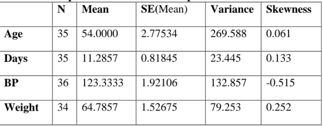
Table 2 Descriptive Statistics before Imputation
N Mean SE(Mean) Variance Skewness
Age 35 54.0000 2.77534 269.588 0.061
Days 35 11.2857 0.81845 23.445 0.133
BP 36 123.3333 1.92106 132.857 -0.515
Weight 34 64.7857 1.52675 79.253 0.252
Clearly from Table 1, at 5% level of significance, Only Y2, Y3 and Y4 are correlated with Y1. Using regression imputation to impute for Y1, it was discovered that regressing Y1 on Y2, Y3 and Y4 yielded a model with a low (adjusted) Coefficient of DeterminationR2 which is very poor for the purpose of prediction and even a high standard error of the estimate. Consequently, Y4 was dropped and a “better” model emerged. Y2, Y3 and Y4 were also imputed using the same procedure. Using Table 1 and considering the (adjusted) R2, we shall have the following imputation models,
𝑌1𝑖 = 𝛽0+ 𝛽1𝑌2𝑖 + 𝛽2𝑌3𝑖 1.6
𝑌2𝑖 = 𝛽0+ 𝛽1𝑌1𝑖 + 𝛽2𝑌3𝑖 1.7
𝑌3𝑖 = 𝛽0+ 𝛽1𝑌1𝑖 + 𝛽2𝑌4𝑖 1.8
𝑌4𝑖 = 𝛽0+ 𝛽1𝑌1𝑖 + 𝛽2𝑌3𝑖 1.9
The parameters were estimated and the following models emerged:
, 𝑌1𝑖 = −31.419 + 0.898𝑌2𝑖 + 0.620𝑌3𝑖 2.0
𝑌2𝑖 = −11.282 + 0.100𝑌1𝑖 + 0.134𝑌3𝑖 2.1
𝑌3𝑖 = 148.860 + 0.190𝑌1𝑖 − 0.519𝑌4𝑖 2.2
𝑌4𝑖 = 118.360 − 0.378𝑌1𝑖 − 0.105𝑌3𝑖 2.3
The Variance Inflation factor (VIF) is an indicator of multicollinearity. It’s an index that measures how much the variance of an estimated regression coefficient is inflated due to multicollinearity. Kutner (2004) suggests that VIF > 5 signifies high multicollinearity. The VIF is given by
VIF = 1/1-R2 2.4 where R2 is the Adjusted coefficient of determination of the model.
For the models in 2.0, 2.1, 2.2 and 2.3, the VIF were computed as 1.278, 1.442, 1.299 and 1.284 respectively. These values are less than 5. So, there was no problem of multicollinearity.
For Y1, there are missing cases in items 3, 7, 17, 25 and 36 and there imputed values are 42, 66,53, 42 and 62 respectively.
The complete dataset from regression imputation included the other variables is tabulated on the Appendix.
For 𝑌1 , the regression model before imputation is given in 2.0 as
𝑌1𝑖 = −31.419 + 0.898𝑌2𝑖 + 0.620𝑌3𝑖
While the regression model after imputation is given by:
𝑌1𝑖 = −38.632 + 0.904𝑌2𝑖 + 0.672𝑌3𝑖2.4 3.1 Stochastic Regression:
Using the normal variates, 𝜀𝑖𝑗 ~N(0,1) generated by the SPSS. We have the following models:
𝑌1𝑖 = −31.419 + 0.898𝑌2𝑖 + 0.620𝑌3𝑖+ 13.784 ∗ 𝜀𝑖𝑗 2.5
𝑌2𝑖 = −11.282 + 0.100𝑌1𝑖 + 0.134𝑌3𝑖+ 4.946 ∗ 𝜀𝑖𝑗2.6
𝑌3𝑖 = 148.860 + 0.190𝑌1𝑖 − 0.519𝑌4𝑖+ 8.660 ∗ 𝜀𝑖𝑗2.7
𝑌4𝑖 = 118.360 − 0.378𝑌1𝑖 − 0.105𝑌3𝑖+ 7.248 ∗ 𝜀𝑖𝑗2.8
The rmse for the imputation models in 2.5, 2.6, 2.7 and 2.8 are 13.820, 4.624, 9.309 and 7.428 respectively. For Y2, the missing cases are in items 6, 23, 26, 30 and 33 and the imputed values are 18.1, 9.6 ,5.1, 8.6 and 9.5 respectively.
The descriptive statistics after stochastic imputation and the new correlation matrix with their significance levels are tabulated below
3.2 Expectation-Maximization.
This technique is stochastic in nature. The imputation models used were those of the regression imputation but with the EM algorithm introducing an error term which is a normal variate, ϵj ~ N(0,1) (not a function of the rmse) Using the EM Algorithm for Missing Value Analysis (MVA)options,we used 25 iterations which is the default number of iterations. This implies that the algorithm estimated the model parameters, then estimated the missing values, then used the filled-in dataset to re-estimate the parameters with the process occurring 25 times before the values converged. The estimates are Maximum Likelihood Estimates
𝑌1𝑖 = −31.419 + 0.898𝑌2𝑖 + 0.620𝑌3𝑖+ 𝜀𝑖𝑗 2.9
𝑌2𝑖 = −11.282 + 0.100𝑌1𝑖 + 0.134𝑌3𝑖+ 𝜀𝑖𝑗 3.0
𝑌3𝑖 = 148.860 + 0.190𝑌1𝑖 − 0.519𝑌4𝑖+ 𝜀𝑖𝑗 3.1
𝑌4𝑖 = 118.360 − 0.378𝑌1𝑖 − 0.105𝑌3𝑖+ 𝜀𝑖𝑗 3.2
3.3 Multiple Imputation.
Graham,et al(2007) recommends at least five imputations. From each analysis, we calculated and saved the estimates.
The overall estimate is the average of the individual estimates.
𝑊
̅̅̅̅ = 1𝑛∑𝑛 𝑊
𝑖=1 I 3.3 Where Wi: i = 1,…,5 are the individual estimates.
For the overall standard error, the within imputation variance as given by 1.4, the between-imputation variance by 1.5 and the total variance by 1.6 were all computed.
Then the overall standard error is the square root of T while a significance test of null hypothesis is performed using the test statistic below
T = √(𝑇)𝑊 ̅̅̅̅ ~t–distribution. 3.4
where𝑊̅ is the average of the estimate and √(𝑇) is the overall standard error. For Y1, the within-imputation variance Ӯ1 = 291.089 and the between imputation variance B1 = 393.243.Therefore, the total variance T1 (as computed using equation 1.6) = 694.163. The overall standard error of Y1 is simply given by (694.416) 1/2 = 26.34697. The total variance and overall standard error of other variables were computed in a similar manner.
Table 3Correlations before Imputation
Age Days BP Weight
Age (P-Value) 1 0.437 (0.016)* 0.575(0.001)** -0.453(0.014)*
Days 0.437(0.016)* 1 0.449(0.011)* -0.233(0.207)
BP 0.575(0.001)** 0.499(0.011)* 1 -0.347(0.060)
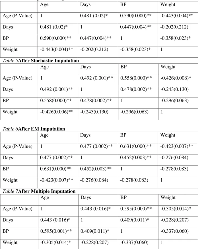
Table 4After Regression Imputation
Age Days BP Weight
Age (P-Value) 1 0.481 (0.02)* 0.590(0.000)** -0.443(0.004)**
Days 0.481 (0.02)* 1 0.447(0.004)** -0.202(0.212)
BP 0.590(0.000)** 0.447(0.004)** 1 -0.358(0.023)*
Weight -0.443(0.004)** -0.202(0.212) -0.358(0.023)* 1
Table 5After Stochastic Imputation
Age Days BP Weight
Age (P-Value) 1 0.492 (0.001)** 0.558(0.000)** -0.426(0.006)*
Days 0.492 (0.001)** 1 0.478(0.002)** -0.243(0.130)
BP 0.558(0.000)** 0.478(0.002)** 1 -0.296(0.063)
Weight -0.426(0.006)** -0.243(0.130) -0.296(0.063) 1
Table 6After EM Imputation
Age Days BP Weight
Age (P-Value) 1 0.477 (0.002)** 0.631(0.000)** -0.423(0.007)**
Days 0.477 (0.002)** 1 0.452(0.003)** -0.276(0.084)
BP 0.631(0.000)** 0.452(0.003)** 1 -0.278(0.083)
Weight -0.423(0.007)** -0.276(0.084) -0.278(0.083) 1
Table 7After Multiple Imputation
Age Days BP Weight
Age (P-Value) 1 0.443 (0.016)* 0.595(0.000)** -0.305(0.014)*
Days 0.443 (0.016)* 1 0.409(0.011)* -0.228(0.207)
BP 0.595(0.001)** 0.409(0.011)* 1 -0.337(0.060)
Weight -0.305(0.014)* -0.228(0.207) -0.337(0.060) 1 * Correlation significant at 5% level of significance.
Table 8Descriptive Statistics before Imputation
N Mean SE(Mean) Variance Skewness
Age 35 54.0000 2.77534 269.588 0.061
Days 35 11.2857 0.81845 23.445 0.133
BP 36 123.3333 1.92106 132.857 -0.515
Weight 34 64.7857 1.52675 79.253 0.252
Table 9Descriptive Statistics after regression Imputation
N Mean SE(Mean) Variance Skewness
Age 40 53.8250 2.49192 248.387 0.078
Days 40 10.9050 0.74744 22.347 0.282
BP 40 123.0000 1.74091 121.347 -0.443
Weight 40 64.5725 1.31076 68.724 0.328
Table 10Descriptive Statistics after Stochastic imputation
N Mean SE(Mean) Variance Skewness
Age 40 53.3250 2.61146 272.789 0.089
BP 40 122.6250 1.97976 126.702 -0.366
Weight 40 64.3800 1.40524 78.988 0.008
Table11Descriptive Statistics after EM Imputation.
N Mean SE(Mean) Variance Skewness
Age 40 53.5750 2.70484 292.646 0.074
Days 40 11.3050 0.80582 25.973 0.138
BP 40 122.8732 1.89100 143.035 -0.410
Table 12Descriptive Statistics after MI imputation
N Mean SE(Mean) Variance Skewness
Age 40 53.33816 26.34697 694.163 -0.0108
Days 40 11.40202 4.89959 24.006 0.1106
BP 40 122.92726 14.40951 207.634 -0.4628
Weight 40 64.70972 12.57911 158.234 0.2428
4.0 DISCUSSION OF RESULTS AND FINDINGS
Regression imputation underestimated the standard error of the four variables as shown in
Table 9, From269.588 to 248.387 for Y1, 23. 445 to 22.347 for Y2, 132.857 to 121.347 for Y3 and 79.253 to 68.724 for Y4 . Also, from Table 4, we see that the P-values in the test for correlation between the variables, Y1, Y2 , Y3 and Y4 are underestimated. At 5% level of
significance, ρ34 was not significant before imputation with P-value of 0.060 but significant
after imputation with a p-value of 0.023. However, at 1% level of significance, ρ14, and ρ23 which were not significantbefore imputation with p-values 0.014 and 0.011 respectively became significantafter imputationwith p-values 0.004 and 0.004. This shows that regression imputation is not robust enough to preserve the relationships among the variables and may lead to Type 1 error – reporting significance in hypothesis testing when there is none. This, of course leads to erroneous inference. Also in Table 9, the changes in values for skewness (a distribution’s departure from symmetry) are very minimal which suggests that there may not be any deviation from the original distribution of the dataset before imputation.
Stochastic imputation underestimated standard errors but not as much as Regression imputation. Table 10 reveals that the variance for the four variables increased. This is clearly due to the introduction of the error term, rmse*ϵijwhere ϵij~ N(0,1) in the models which increases the variability in the dataset. Table 5 shows that at 5% level of significance the statistical relationships are preserved. However, at 1% level of significance, ρ21, ρ32 and ρ41 which were not significantbefore imputation with p-values 0.016, 0.011 and 0.014 respectively became significantafter imputation.with p-values 0.001, 0.002 and 0.006 respectively. Also, changes in values for skewness are not much as shown in Table 10.
EM imputation only records a slight underestimation of standard errors. A study of Tables 8 and 11 reveals the underestimation after EM imputation as follows: 2.77534 to 2.70484, 0.81845 to 0.80582, 1.92106 to 1.89100 and 1.52675 to 1.50293 for S.E(Y1), S.E(Y2), S.E(Y3) and S.E(Y4) respectively. This underestimation is very minimal and Table 6 shows that relationships at 5% level of significance are still maintained. This verifies the claim of Enders, C.K. (2010) that “EM imputations preserve the relationships with other variables, which is extremely vital if the researcher is going into Factor Analysis and Regression.” Interestingly, at 1% level of significance as revealed in Table 6 , ρ12, ρ23 and ρ14 which were not significantat 5% became significant with with p-values 0.002, 0.007 and 0.003 respectively. The skewness for the four variables remains almost the same with the ones before imputation. From 0.061 to 0.074 for Y1, 0.133 to 0.138 for Y2, -0.515 to -0.410 for Y3 and 0.252 to 0.242 for Y4. These values are close to zero showing that their distributions still remain approximately symmetric.
Multiple imputation, MI is the only technique that preserved the relationships of the variables both at 5% and 1% levels of significance. This is evident in Table 7. This makes it “better” than the EM technique especially in studies where the statistical relationships amongst the variables are paramount. A study of Table 12 reveals that there is no underestimation of standard errors rather they were inflated. The S.E.(Y1) moved from 2.77534 to 26.43697, 0.81845 to 4.89959 for S.E.(Y2), 1.92106 to 14.40951 for S.E.(Y3) and 1.52675 to 12.57911 for S.E.(Y4). This could be a disturbing development when testing hypotheses about the variables especially for Y1 which records the highest margin. Clearly, MI doesn’t underestimate standard errors but may create the problem of Type II error- not reporting significance when they actually exist. Now, because of the inverse relationship between the probability of Type II error, β and statistical power (1- β), we can say that the MI has not been able to appropriately tackle the issue of reduced power in this case. Though, some statisticians would rather risk Type II error than Type I error because in hypothesis testing, the practice is usually to consider Type I error more seriously than Type II error. In other words, any technique that would minimise Type I error would surely be preferred.
Once again, values in skewness did not change significantly showing that the distribution of the dataset is still maintained. The results of MI done well are unbiased parameter estimates and no underestimation of standard errors and P-values. However, MI created by an incorrect model can lead to erroneous decisions.
Descriptive statistics before Imputation Descriptive statistics after MI N Mean SE(Mean) Variance Skewness N Mean SE(Mean) Variance Skewness
Age 35 54.0000 2.77534 269.588 0.061 40 53.33816 26.34697 694.416 -0.0108
Days 35 11.2857 0.81845 23.445 0.133 40 11.40202 4.89959 24.006 0.1106
BP 36 123.3333 1.92106 132.857 -0.515 40 122.92726 14.40951 207.634 -0.4628
Weight 34 64.7857 1.52675 79.253 0.252 40 64.70972 12.57911 158.234 0.2428
5.0 Conclusion
The existence of missing data creates problems that can never be completely solved but managed using some good imputation techniques.
The underestimation of standard errors and P-values are highest in the regression technique, moderate in the stochastic, minimal in the EM technique and inflated in the MI. At 5% level of significance, correlations were maintained only by the EM and the MI techniques with only the MI still maintaining correlations at 1% level of significance but with inflated standard errors, exposing the researcher to the risk of Type II error. Unlike Multiple Imputations, the regression imputation, stochastic imputation and EM techniques are not robust enough to preserve relationships among variables at 1% level of significance. These techniques should be dropped in vital statistics, epidemiology, and government budgeting where most decisions are based on hypothesis testing at 1% level of significance
An attempt to compare these techniques shows that none of them is universally better than the other. While regression, stochastic and the EM were relatively better than the MI in maintaining the distribution of the original dataset. MI performed better than them in maintaining the relationships. Some underestimate standard errors and P-values thereby creating the problems of Type I error while others like the MI inflate standard errors and P-values, creating the problem of Type II error.
The EM has the advantage that even when the assumption of multivariate normal distribution of observations is in error, the algorithm seems to work remarkably well. But because it still underestimates standard errors, it is only advisable if the percentage of missing data is under 5%. Enders (2010)
Luengo, et al (2011) suggested that the EM and the MI techniques should be adopted in fields of knowledge like Bioinformatics, Climatic science and Medicine.
However, there is no universal imputation technique that performs ‘best’ for all cases. It all depends on the objectives of the researcher.
6.0 References
Brick, M. and Kalton, G., (2000), “Weighting in household panel surveys”, Researching social and economic change: the uses of household panel studies, ed Rose, D., Routldege, London.
Everitt, B.S. (2002), “The Cambridge Dictionary of Statistics 2nd Edition”. Institute of psychiatry, kings College, University of London.
Fellegi, I. P, and D. Holt (1976), “A Systematic Approach to Automatic Edit and Imputation”,
Journal of the American Statistical Association, 71, pp. 17-35.
Graham J. W., Olchowski A. E., and Gilreath T. D., (2007). “How many imputations are really needed?” Some practical classifications of multiple imputation theory.
Howell, D.C (2008), “The analysis of Missing data handbook of Social science Methodology”, London.
Julian, L., Salvador, G., and Francisco, H. (2011), “On the choice of best imputation methods for missing values considering three groups of classification methods”. Springer-Verlag London limited.
Kutner, M. H., Nachtsheim C.J., Neter, J., (2004), “Applied Linear Regression Models”, 4th Edition. Mc Graw Hill Irwin
Little, R.J.A, and Rubin, D.B.(2002), “Statistical Analysis with Missing Data”, 2nd
edition.
New York: John Wiley.
Pickles, A. (2005), “Missing data, problems and solutions”, Kimberly Kempf-Leonard (ed.),
Encyclopedia of Social Measurement. Amsterdam: Elsevier 689–694.
Schaeffer, J.L. and Graham, J.W. (2002). “Missing data: Our view of the state of the art”. Psychological Methods 7.
Schafer, J.L. (1997) , “Analysis of Incomplete Multivariate Data” London: Chapman & Hall, London. (Book No. 72, Chapman & Hall series Monographs on Statistics and Applied Probability.)
Von, H., and Paul, T., (2007) , “Regression with missing Y’s: an improved strategy for analysing multiple imputed data. Sociological Methodology.
More information about the firm can be found on the homepage: http://www.iiste.org
CALL FOR JOURNAL PAPERS
There are more than 30 peer-reviewed academic journals hosted under the hosting platform.
Prospective authors of journals can find the submission instruction on the following page: http://www.iiste.org/journals/ All the journals articles are available online to the readers all over the world without financial, legal, or technical barriers other than those inseparable from gaining access to the internet itself. Paper version of the journals is also available upon request of readers and authors.
MORE RESOURCES
Book publication information: http://www.iiste.org/book/
Academic conference: http://www.iiste.org/conference/upcoming-conferences-call-for-paper/
IISTE Knowledge Sharing Partners
EBSCO, Index Copernicus, Ulrich's Periodicals Directory, JournalTOCS, PKP Open Archives Harvester, Bielefeld Academic Search Engine, Elektronische Zeitschriftenbibliothek EZB, Open J-Gate, OCLC WorldCat, Universe Digtial Library , NewJour, Google Scholar