Defect Prediction on the Hardware Repository - A Case Study on the OpenRISC1000 Project

(1)

D

EFECT

P

REDICTION ON THE

H

ARDWARE

R

EPOSITORY

-

A

C

ASE

S

TUDY ON THE

O

PEN

RISC1000

P

ROJECT

SILVIU MUSA

A THESIS SUBMITTED TO THE FACULTY OF GRADUATE STUDIES

IN PARTIAL FULFILLMENT OF THE REQUIREMENTS FOR THE DEGREE OF

MASTER OF APPLIED SCIENCE

GRADUATE PROGRAMME IN ELECTRICAL ENGINEERING AND COMPUTER

SCIENCE

YORK UNIVERSITY

TORONTO, ONTARIO

MARCH 2017

(2)

Abstract

Software defect prediction is one of the most active research topics in the area of mining software engineering data. The software engineering data sources like the code repositories and the bug databases contain rich information about software development history. Mining these data can guide software developers for future development activities and help managers to improve the development process. Nowadays, the computer-engineering field has rapidly evolved from 1972 until present times to the modern chip design, which looks superficially and very much like software design. Hence, the main objective of this thesis is to check whether it would be possible to apply software defect prediction techniques on hardware repositories. In this thesis, we have applied various data mining methods (e.g., linear regression, logistic regression, random forests, and entropy) to predict the post-release bugs of OpenRISC 1000 projects. We have conducted two types of studies: classification (predicting buggy and non-buggy files) and ranking (predicting the buggiest files). In particular, the classification studies show promising results with an average precision and recall of up to 74% and 70% for projects written in Verilog and close to 100% for projects written in C.

(3)

Acknowledgements

I would like to thank my supervisor Prof. Mokhtar Aboelaze for the support, guidance, and feedback which has helped me pursue my MSc. Equally, I would like to thank my co-supervisor Prof. Zhen Ming (Jack) Jiang for extensively using his time to provide me the best of guidance and support during this project. I am very grateful to Mr. Jeremy Bennett (Open Cores community) for providing all the needed additional information. My inexpressible appreciation goes to my family and friends. Their unconditional love and support have always been the main source of motivation in my personal and professional life. I would also like to thank the entire Graduate Studies Department of the Electrical Engineering and Computer Science at York University for making my master studies a wonderful experience.

(4)

List of Tables

Table 1: Soft core processors ... 4

Table 2: HDL-Complexity Metrics ... 20

Table 3: C language – Complexity metrics... 21

Table 4: Complexity metrics summary for Mor1kx and Or1k-sim ... 24

Table 6: Released versions for Mor1kx project ... 32

Table 7: Mor1kx HCT metrics summary ... 33

Table 8: Released versions for Or1k-sim project ... 33

Table 9: Classification table... 36

Table 10: The prediction of the Mor1kx (Verilog) experiment built using the logistic regression prediction model - Precision ... 37

Table 11: The prediction of the Mor1kx (Verilog) experiment built using the logistic regression prediction model - Recall ... 37

Table 12: The prediction of the Mor1kx (Verilog) experiment built using the logistic regression prediction model - F-Measure ... 38

Table 13: The prediction of the Mor1kx (Verilog) experiment built using the random forest prediction model - Precision ... 40

Table 14: The prediction of the Mor1kx (Verilog) experiment built using the random forest prediction model - Recall ... 40

(7)

Table 15: The prediction of the Mor1kx (Verilog) experiment built using the random

forest prediction model - F-Measure ... 41

Table 16: The prediction of the Or1k-sim (C) experiment built using the logistic regression prediction model - Precision ... 44

Table 17: The prediction of the Or1k-sim (C) experiment built using the logistic regression prediction model - Recall ... 45

Table 18: The prediction of the Or1k-sim (C) experiment built using the logistic regression prediction model - F-Measure ... 46

Table 19: The prediction of the Or1k-sim (C) experiment built using the random forest prediction model - Precision ... 47

Table 20: The prediction of the Or1k-sim (C) experiment built using the random forest prediction model - Recall ... 48

Table 21: The prediction of the Or1k-sim (C) experiment built using the random forest prediction model - F-Measure ... 49

Table 22: Mor1kx – Spearman correlation coefficient ... 53

Table 23: Or1k-sim – Spearman correlation coefficient ... 54

Table 24: Mor1kx – Linear regression - Root relative squared error ... 56

Table 25: Or1k-sim – Linear regression – Root relative squared error ... 56

Table 26: Mor1kx – Entropy of modified files ... 58

(8)

List of Figures

Figure 1: OpenRISC1000 – Component blocks diagram ... 6

Figure 2: Functional Blocks for OR1200RTL ... 9

Figure 3: Our process to mine the OpenRISC1000 hardware repository ... 17

Figure 4: An example of code commit logs ... 25

Figure 5: Code commits and according version ... 26

Figure 6: Example of a .csv file ... 28

Figure 7: Mor1kx – HCT set of metrics... 29

Figure 8: Mor1kx – UnderstandSCI set of metrics ... 30

Figure 9: Example of a csv file for a file written in C ... 31

Figure 10: Weka – The Explore Interface... 31

Figure 11: Mor1kx – Precision ... 42

Figure 12: Mor1kx – Recall ... 42

Figure 13: Mor1kx - F-Measure ... 43

Figure 14: Or1k-sim- Precision ... 50

Figure 15: Or1k-sim Recall ... 50

Figure 16: Or1k-sim F-Measure ... 51

Figure 17: Mor1kx- Linear Regression - Spearman correlation coefficient ... 57

(9)

Figure 19: Entropy .csv file example ... 60 Figure 20: Mor1kx- Comparison between linear regression (LR) and linear regression on entropy ... 61 Figure 21: Or1k-sim - Comparison between linear regression and linear regression on entropy ... 61

(10)

Chapter 1 Introduction

The hardware development complexity is exponentially increasing nowadays; a single scale of chips may contain multiple billions of transistors [25]. The growing design complexity requires efficient hardware quality assurance (QA) techniques that differ from the software QA. A major difference between software and hardware QA process is that the hardware QA is not done sequentially, the different functional blocks behave simultaneously making the QA process more difficult. Generally, two thirds of the total hardware design budget is used for design QA [2, 21]. Meanwhile, there is an increasing number of projects that were written using a hardware description language (e.g., VHDL). Hence, it would be worthwhile to investigate whether some of the software QA techniques would be applicable to the process of hardware QA.

One of the active research areas in software engineering is software defect prediction. Software Defect Prediction (SDP) is the line of research that is concerned with building prediction models, which leverage software metrics to predict defect-prone areas within a software system. The typical metrics include code complexity metrics (e.g., lines of code) or historical code change metrics (e.g., code churns). Together with the traditional software testing approach, the data obtained from SDP can be used to further improve the quality of various software systems. It would be worthwhile to

(11)

investigate whether the software prediction techniques can be applied to detect potential issues in the hardware code.

With respect to applying SDP on hardware repositories, there is only one recent work [21] which predicts hardware defects on one large-scale commercial product. However, there are no published works on predicting defects on open source hardware repositories. Hence, this would be the focus of this thesis.

This thesis contains the defect prediction work done over a very popular open hardware project and open source development OpenRISC1000. Our goal was to perform an empirical investigation on this hardware project studying the relationship between various metrics (e.g., code complexity metrics and historical change metrics) and the post-release bugs. By applying the SDP techniques on hardware repositories, we were able to find the defect prone software modules. We focused on the post-release bugs rather than pre-release bugs or all bugs because of the post-release bugs, which are bugs discovered after the systems are released into the field, are more important with respect to the customer experience.

Thesis Organization

This thesis is organized as follows: Chapter 2 presents the OpenRISC1000 project and the background information about the SDP process. Chapter 3 provides an overview of our case study. Chapter 4 describes our experiments and discusses our results. Chapter 5 concludes this thesis and presents some future work.

(12)

Chapter 2 Background and Related Works

This chapter is organized as follows. First, we will describe the open source OpenRISC1000 project in Chapter 2.1. Then we will provide an overview of the related works in the area of SDP in Chapter 2.2.

2.1 OpenRISC1000 Overview

Since 1960, the embedded computers have evolved continuously as a result of the advances in the design and manufacture of microelectronic components and devices. Starting 1980, there is a new architectural approach regarding microprocessors, favouring a reduction in design complexity [12, 23].

The Reduced Instruction Set Computing (RISC) is a type of microprocessor architecture that utilizes a small, highly-optimized set of instructions, rather than a more specialized one, often found in other types of architectures. The most important characteristics of this family of processors are: one cycle execution time, pipelining and a large number of registers [2].

Almost in the same period of time (mid 80’s) when the RISC architecture was designed, there was a movement in terms of open source and free software systems. The Free Software Foundation was born aiming to create the environment for less restrictive software regarding freedom to access and open of suffocating “usage protective measures” [1]. Fifteen years later, the philosophy was transferred to the discipline of

(13)

hardware design. As a result, a large number of soft cores are currently available as open hardware. Cortex-M1, OpenRISC1000, OpenSPARC, LEON, Lattice Micro32, RISC-V are only a few of names from the list. The most popular of open source hardware systems are presented below.

Processor Developer Processor Developer

AEMB Shawn Tan Nios I, Nios II Altera

ARC ARC International OpenFire Virginia Tech

Cortex-M1 ARM OpenRISC OpenCores

ERIC5 Entner Electronics OpenSPARC SUN

eSI-RISC EnSillica T1 SUN

JOP Martin Schoeberi PacoBlaze Pablo Bleyer

Lattice Micro32 Lattice pAVR Doru Cuturela

LEON2 ESA PicoBlaze Xillinx

LEON 3/4 Aeroflex Gaisler RISC-V UC-Berkeley

MOL86 MicroCore Labs SecretBlaze U of Montpellier

Navre Seb Bourdeauducq

Table 1: Soft core processors [24]

In 1990, one of the most prominent projects aiming to develop an open source processor architecture was initiated by a group of students. These students had the goal to create a RISC processor design, including specifications and implementation. The name

(14)

of the project was OpenRISC1000 and, at the same time, an online open source hardware design community called Open Cores was created.

The Open Source Hardware Community, known as Open Cores Community has more than 150,000 registered users [3]. There are 20 programmers assigned to be the maintainers of the project and the most popular names are: Damjan Lampret, Julius Baxter, Jeremy Bennett, and Stefan Kristiansson.

In the absence of a widely accepted open source hardware license, the components produced by the Open Cores initiative used initially several different software licenses. The Open Cores portfolio consists of multiple design elements from central processing units, memory controllers, peripherals, motherboards, and other components. The cores are implemented in the hardware description languages like Verilog, VHDL which may be synthesized to either silicon or gate arrays. Among the components created by Open Cores contributors are: OpenRISC1000 - a highly configurable RISC central processing unit, Amber (processor core) - an ARM-compatible RISC central processing unit, a ZilogZ80 clone, USB 2.0 controller, Tri Ethernet controller, 10/100/1000 Mbit. From the multitude of Open Cores community achievements, the OpenRISC1000 project has the largest popularity [13].

2.1.1 OpenRISC1000 Architecture

OpenRISC1000 is an open source 32-bit processor IP core that has been widely used in many academic and technologic projects [5]. Its nickname is OR1K and the project is one important component of ORP “Open RISC reference platform”.

(15)

OpenRISC1000 provides a large area of implementations at a multitude of price per performance levels for a large range of industrial and telecommunication applications [20]. The basic implementations of the processor will only occupy 70% of a 50,000-gate Xilinx Virtex FPGA board, running at 80 MHz, reaching 80 MIPS.

The microprocessor block components are described in detail by Pablo Sanchez and Eugenio Villar in their paper “Using Open Source Cores in Real Applications” as being a 32/64-bitload microprocessor with store RISC architecture that has been designed with the emphasis on performance, simplicity, low power requirements, scalability and versatility [24]. The main CPU unit is implemented in 15,400 System C code lines (Figure 1) and has the following components described below according to the official manual [24].

(16)

The Integer Unit is the main part of the CPU designed to decode each instruction, to obtain the operation code and the operands. After each operation is performed, the integer unit writes the existing results. The integer unit is designed to allow the utilization of a higher clock frequency. The System C description of these units has 4,100 code lines.

Data and instruction caches are separate modules according to the hardware architecture of the design and are highly configurable. Cache size can be set from2 KBto8 KB and data block size can be set to 16, 32 or 64 bytes. Least Recently Used (LRU) is the algorithm used and it proved to be very efficient. This unit is described in 5,900 System C code lines.

Exception management unit is designed to calculate the address where the exception handler routine is placed and to decide which information about the status of the core must be stored for later restoring of the execution. This unit is described in 600 System C code lines.

Debug unit and development interface is an optional block that provides the possibility to create hardware breakpoints based on comparison conditions with stored or loaded values, data and instruction memory addresses. This unit is very closely related to the development interface which allows the debugging process to be completely in-system. Through the development interface, the debugging software can analyze the status of the CPU the memory content and trace information. The debug and development interface description takes 2,600 System C code lines.

(17)

Programmable interrupt controller allows the connection of 32 external masked interrupt lines through the interrupt line provided by the architecture. The OpenRISC1000 architecture only provides an insufficient number of interrupt thus a programmable interrupt controller (PIC) has to be implemented.

Tick timer facility provides the software with a precise clock reference. The tick timer generates an interrupt when the count reaches a programmed value.

Performance counters unit keeps a count of the number of times that a certain event has occurred. These events can be: instruction fetches, load and store accesses, cache misses and watch points.

Power management unit helps to better administer the power consumption of the core. This unit can perform modifications of the system clock frequency; it can shut down modules or can force the CPU to enter sleep mode.

Watchdog unit is used to prevent the CPU from entering into an endless loop or an erroneous routine from which the system cannot recover from.

(18)

The functional blocks are presented in the Figure 2. All of these blocks were designed with the focus on several principles such as ergonomics, efficiency, and lower power consumption [17].

The project started in 1998 aiming to develop reusable IP cores processors in Verilog/VHDL and since then each project has had several hundreds of code commits. First edition was launched in 2000 and since then up to the present times has been regularly updated to reflect the state of the latest implementations. The statistics provided by the Open Cores community show a total of 1,093 downloads per year. The project is known now as Design proven, ASIC proven, FPGA proven, but it is well known that still suffers historically from a lack of testing [24]. Knowing the increasing trend of design reuse, the developed IP cores have a high probability to be used in the research industry

(19)

for the embedded control systems and fast FPGA prototyping and they can be implemented as well for day by day use. There are already a few examples of real implementations that have become a market success: Samsung DTV, Allwiner power controllers, and NASA for the control of TechEdStad.

2.1.2 OpenRISC1000 Repository Structure

OpenRISC 1000 project can be considered as a showcase of an open, modular standard specification geared towards real hardware implementations. The code for all projects in the OpenRISC IP Core family, such as OpenRISC1000, OpenRISC1200, and other builds, is combined into a single source tree and is hosted by the most popular web-based Git repository service GitHub (https://github.com/openrisc). The tree contains the complete source code for all the modules including project builds for each supported Operating System (OS) platforms. Linux is the main platform and the biggest parts of the project developments were done for it. In addition, the project has also been ported to Real Time Operating Systems like freeRTOS, RTEMS, and eCOS.

To fork all the OpenRISC repositories to a personal GitHub account and to download them to the local computer was the first mandatory step in our study. The complete project family, including compilers, tool chains, simulators and existing builds has a size on disk very close to 10 GB with 726,134 files and 47,543 folders. Most of the code was written in the Verilog, and C programming languages. Both languages have concepts of components, functions, methods and modules like any other standard programming languages.

(20)

The most important directories of the repository are the following:

• Mor1kx is a modular source base, the most recent version of the OR1K project.

Mor1kx core is intended to replace the existing current OpenRISC1200 version. Mor1kx comes with 3 main configurations: Pronto-core is the configuration having three stages “delay-slot-free” and does not have a memory management unit (MMU); Espresso-core has a three-stage pipeline and does not have a MMU as well; Cappuccino-core has 6-stage pipeline and it can have MMUs and caches, which make it powerful enough to run Linux.

• ORPSoc is an OpenRISC reference platform (System on Chip) for further OS

development. The trend is towards standard software distributions.

• OpTiMSoc is a tiled multi-core platform included in the OpenRISC project. The

project can run on big FPGA boards.

• Or1k-gcc is the OR1KX Gnu collection compiler. Or1k-src it is a part of the tool

chain containing the binutils and GDB libraries.

• Or1ksim is the official emulator for the Or1k project and is built as a single core.

• Jor1k is a JavaScript simulator written in Java.

• UClibc-or1k contains the uClibc embedded C libraries.

• LLVM-Or1k (Low Level Virtual Machine for Or1k) contains the preliminary

support in LLVM and LINUX.

Each of the above-presented modules is hosted by GitHub as individual projects and each project can have up to 13 versions. The main branch is the one that accepts the

(21)

current code commits. The testing is done using the mentioned simulators Orksim and Jor1k and Verilator (Verilog to System C) the dedicated testing tool made by the largest FPGA producer Xilinx. Using the existing results of the past testing activity and considering the limitations of resources in the software industry, it is very valuable to exactly predict the areas which are prone to failures in order distribute those resources properly to ensure the best results on launching software products.

By analyzing the existing data contained in the above systems, we can obtain valuable perspectives over their development processes [8, 18]. The large open software and hardware systems are increasingly important in the daily lives, and the software programming errors are affecting professionals at all levels. Hence, it is very important to have an exploratory study over a large project in order to demonstrate how the collected data and all the existing information on an open hardware project can help us to obtain even more knowledge and information.

2.2 Software Defect Prediction

A software defect, commonly referred as a “software bug” can be defined as an issue or deficiency in the software product which causes it to perform in an unexpected way [22]. Since defects in software can lead to malfunctioning of the system, which could in some cases affect the overall quality of the project, the general objective of software QA and validation activities is to release software with no known defects. Trying to achieve this goal, all the unexpected malfunctions are reported and documented in the defect database also known as online bug repository for the open source projects

(22)

[22]. All defects found during the software QA and validation activities become records of the repositories in a pre-defined format, often with the sole purpose of facilitating their resolution. Such repositories, which are usually accessible online, are generally called the bug repositories, or issue tracking repositories [4, 29].

The online databases usually provide the platform where worldwide programmers and testers can access the information about defects of their interest. They can add, edit, or update the information related to a given defect or comment, provide expertise or guidance to help resolve the defect, and track the progress of reported defects and monitor their statistics. To facilitate the documentation and exchange of information, various attributes are recorded for each reported defect. Some of these attributes are mandatory aimed at providing the basic information pertaining to given defect, while others are optional that provide additional details.

The most commonly used software QA and validation approach is software testing [26, 19]. Software testing verifies the behavior of the software system by executing the test scenarios and checking its runtime behavior against the specification. In addition to software testing, recently SDP is another complementary approach which can be used to reveal potential problems in a software system.

Software Defect Prediction (SDP) is an area of research that focuses on building prediction models, which use software metrics to predict defect-prone areas of a software system [28]. SDP uses various metrics extracted from the source code, the historical revisions, as well as the bug repositories [31].

(23)

There are many existing works in the area of SDP. For details please refer to [11]. We describe here the two pieces of works which are most relevant to this thesis.

1. The ways to practically identify and prioritize defects are addressed in multiple research papers in the software defect prediction field, including the one written by Zimmermann and Zeller, “Predicting Defects for Eclipse” [32]. This paper is the first work and proposes the idea of mining an open source, publicly available software repositories to predict potential defects.

2. Regarding mining hardware repositories, there is only one published work. It is written by Parizy, Takayama, and Kanazawa, called “Software Defect Prediction for LSI Designs” [21]. This is a study that was developed by Fujitsu Laboratories aiming to predict software defects by mining hardware repositories. This study was done in the industry using proprietary software defect database and proprietary hardware repositories focusing only on entropy studies.

However, there are no existing works which predict defects on open source hardware repositories. Hence, the current state of the research in the field gives us the opportunity to bring our contribution.

In this thesis, we have made a first empirical study on predicting bugs from open source hardware repositories. We have used OpenRISC1000 project and proceeded in our work using the existing state of the art methods and trying to see if there are better ways to leverage the software metrics. Although Parizy et al. [21] also studied the projects written in the Verilog language, they only applied the entropy as their prediction

(24)

techniques. In this work, in addition to the entropy studies, we have used several other data mining techniques (e.g., regression and random forests) to predict the hardware defects.

(25)

Chapter 3 Case Study Overview and Setup

In this chapter, we describe our process of applying SDP techniques to predict potential defects in the hardware repositories. In particular, we explain the setup and the tools used in our case study.

3.1 Overview

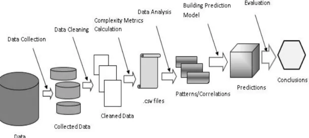
The main objective of this thesis was to apply the SDP technique to a hardware repository. In this study, we picked OpenRISC1000 as our case study project. In order to achieve this objective, similar as described in Zimmermann and Zeller paper [31], our process consisted of five steps as illustrated in Figure 3: (1) data collection; (2) data cleaning; (3) complexity metrics calculation; (4) building prediction model; and (5) evaluation.

(26)

Figure 3: Our process to mine the OpenRISC1000 hardware repository

(1) During the data collection step, the historical data from the online OpenRISC1000 open source repository was extracted. There were two types of historical data in our study:

i. the GitHub repository, which contains the past revisions of the OpenRISC1000 source code; and

ii. the BugZilla database, which contains the reported defects for various releases of the OpenRISC1000 projects.

(2) During the data cleaning step, the unnecessary data was removed and the input data was converted into the desirable format which can be processed by the subsequent tools. (3) During the complexity metrics calculation step, various complexity metrics were calculated for different releases of the software system. These complexity metrics were used in the later data mining models to predict the potential defects in the source code. Since there were two types of programming languages used in the OpenRISC1000

(27)

project, the Verilog and C. Hence, different types of complexity metrics were calculated for these two different programming languages.

(4) During the data analysis step, we studied the relationship between various code metrics with the bugginess of the systems. In particular, we explored the correlations between the complexity metrics and the past bug history.

(5) During the building prediction model step, various prediction models were built using the calculated complexity metrics as well as the past defect history. In particular, in this thesis, we studied two types of prediction models, classification, and ranking. For classification, we used two methods: logistic regression and random forest in order to determine which one provides better results. For ranking, we used the linear regression method.

(6) During the Evaluation step, the effectiveness of the prediction models was evaluated. In particular, we wanted to check whether the prediction models can be used to prediction bugs on the future releases of the systems.

3.2 Setup

There are three aspects related to the case study setup: (1) data download; and (2) the tools for complexity metrics calculation; and (3) the tool for building the prediction models.

(28)

3.2.1 Data Download

For the case study, we used two main sources of data available for the OpenRISC1000, the project repositories and the associated Bugzilla online database. Both were forked from the official location to a personal GitHub account and successfully downloaded to the local machine. For the hardware repository, the size of the download was approximately 9 GB. For Bugzilla online database, the size was around 70 MB.

3.2.2 Tools for Complexity Metrics Calculation

After collecting all the necessary data related to the study, the complexity metrics calculation phase naturally came next in the working flow. Software analysis generally extracts arbitrary properties of software source code. Software metrics provides various insights on various characteristics of the source code. Classic software metrics range in a large variety, from the very simple Source Lines of Code (SLOC) to more complex measures such as Cyclomatic Complexity measurements. Typical metrics report provides details on individual modules and summaries for subsystems. Such metrics are widely used to judge the quality or the complexity of source code.

The main advantages of using well-defined complexity metrics are their wide acceptance, unbiased assessment of source code quality, repeatability of measurements, ease of measurement, and the ability to judge progress in enhancing quality by comparing before and after assessments.

(29)

We built the bug prediction models using the complexity metrics guided by the thought that the most complex code would result in more bugs. However, as there were various complexity metrics proposed, our goal was to collect as many complexity metrics as possible when building the prediction models.

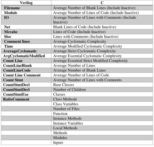
Since there were two types of programming languages in the OpenRISC1000 project, the Verilog and C, we used the HDL tool [16] to calculate the complexity metrics for the Verilog code and the UnderstandSCI [27] tool to calculate the complexity metrics for the C code.

The Hardware Description Language (HDL) Complexity Tool parses the Verilog code and calculates the code complexity metrics (Table 2).

Name Description

Filename the name of the file

Module the name of the module

IO input output elements Net design elements McCabe cyclomatic complexity Sloc lines of code

Comment lines lines containing comments

Time propagation time

Table 2: HDL-Complexity Metrics

The UnderstandSCI tool is a static analysis tool focused on source code comprehension and software metrics. The UnderstandSCI tool was widely used in various projects [16]. We used the UnderstandSCI tool to calculate the code complexity metrics for the C code. The following (Table 3) metrics were calculated:

(30)

Name Description

Average Number of Blank Lines (Include Inactive)

the average number of lines that are not containing code

Average Number of Lines of Code (Include Inactive)

the average number of lines that are containing code

Average Number of Lines with Comments (Include Inactive)

the average number of lines that are containing comments

Blank Lines of Code (Include Inactive) the number of lines that are not containing code Lines of Code (Include Inactive) the total number of lines of code

Lines with Comments (Include Inactive) the total number of lines that are containing code

Average Cyclomatic Complexity the number of linearly independent paths through a program's source code

Average Modified Cyclomatic Complexity the average of the modified number of linearly independent paths through a program's source code

Average Number of Lines the average number of lines Average Number of Blank Lines the average number of blanc lines Average Number of Lines of Code the average number of lines of code

Base Classes the number of classes from which other classes are derived

Number of Children the total number of direct subclasses

Classes the total number of classes

Class Methods the total number of methods

Class Variables the total number of variables defined in a class Number of Files the total number of files

Function the total number of functions Instance Methods the total number of subroutines

Instance Variables the total number of variables defined in a class Local Methods the total number of local methods

Methods the total number of methods

Modules the total number of modules

Program Units the total number of program units Subprograms the total number of subprograms

Table 3: C language – Complexity metrics

3.2.3 The Tool for Building the Prediction Models

We used the Waikato Environment for Knowledge Analysis (WEKA) as our tool to build the bug prediction model. WEKA is a machine learning workbench currently

(31)

being developed at the University of Waikato. Its purpose is to allow users to access a variety of machine learning techniques for the purposes of experimentation and comparison using real world datasets. A workbench represents a set of tools bound together by the same user interface and each of these represents an individual program. The machine learning tools are written in a variety of programming languages (C, C++ and LISP). The last version of WEKA application includes multiple machine learning capabilities [10]. By providing the option to build a data mining model based on a training dataset, Weka has proven to be the ideal tool for our study.

(32)

Chapter 4 Experiments

In this chapter, we present our experiment on prediction bugs for the OpenRISC1000 project. The experiment was performed on a Dell XPS, I7-3770K single core desktop computer with 16 GB of RAM and 1 TB hard disk drive storage capacity.

4.1 Data Collection

4.1.1 The Hardware Repository

For this study, we used two main sources of available data for the OpenRISC1000, the project repositories and the associated Bugzilla online database. A total of 9.06 GB was downloaded to the local machine.

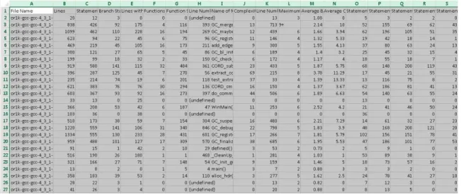
By looking through the downloaded data, we understood that this project started in 2001 and it is still ongoing at the present time. In total, there were 28 components/sub-projects inside the OpenRISC1000 project. Within these 28 sub-components/sub-projects, there were more than 635,127 files overall. In total, there were more than 183,344,000 lines of code and 87,768,000 of statements for the entire project. Among them, 15,655 lines of code contained in 529 files were written in Verilog. The rest of 634,598 files containing 183,328,345 lines of code were written in C.

From all the OpenRISC1000 component sub-projects, we selected for our study only those that had multiple released versions in order to make possible future

(33)

comparisons. As a result, only 2 sub-projects fulfilled this condition. To have a balanced study, we selected Mor1kx, the actual processor design written in Verilog, and Or1k-sim, the current simulator of the processor, written in C.

Table 4: Complexity metrics summary for Mor1kx and Or1k-sim

4.1.2 Bugs Collection

A copy of the project’s post-release bugs was obtained from the online OpenRISC1000 Bugzilla Database. This database collects all the reported issues and modification requests that are submitted electronically by worldwide users. They are commonly referred to as “bug reports”. This term is quite misleading as not all reported issues are defects, as some of the reported issues are just requests for optimization, or suggestion for different future improvements. Normally, every bug report should contain a variety of supporting meta-information such as a unique identification number, the software version, and the operating system it relates to, or the reporter’s perceived

importance. In addition, the entries should contain a short one-line summary of the issue at hand, followed by a more elaborate description. In our case, the additional information was missing for some of the reported bugs. Considering also the fact that the number of reported issues present in the database (106 instances in total) was too small to be used in the data mining study, we had to consider the second solution. Hence, we examined the

Verilog C

Mor1kx Or1k-sim

529 files 2,063 files

(34)

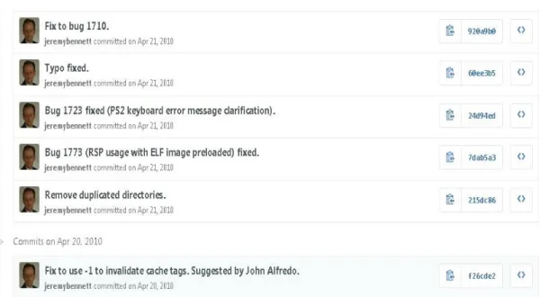
commit logs of the online code repositories. Methodically, we analyzed all the existing logs of the code commits and we included the code revisions whose commit logs contained the words like “corrections” or “fixes”. Usually, when the developers submit their code, they usually include some short messages, called the commit logs, which contain the purpose of their submission. For example, if their code commit is for fixing some bugs, their commit log might contain phrases like “fixed 1067” or “bug #1025”. Figure 4 shows an example.

Figure 4: An example of code commit logs

We built a group of large spreadsheets for each sub-project containing the list of bugs, the patch for each modified file when fixing that bug and the date when the code commit was submitted.

(35)

Knowing the release date for each version and the date when each code commit was submitted, we checked and ensured that all the software defects were post-release bugs. Post-release bugs refer to bugs reported after that version of the system is released. We also took into consideration the existing comments inside the code commits. In this thesis, we focus on analyzing and predicting the post-release bugs is because these are the bugs which escape from software testing and can potentially impact the customer experience.

Figure 5: Code commits and according version

4.2 Data Cleaning

The second step in our data processing process is data cleaning. We verified if the data values were correct and conform to the existing dataset of rules. The non-useful information such as the “author” and “submission date” fields was removed. In this way, the existing data was prepared to be used for in depth analysis.

(36)

4.3 Complexity Metrics Calculation

Using the UnderstandSCI and HCT tools, we were able to extract from the analyzed repositories all the useful complexity metrics [6].

Verilog C

Filename Average Number of Blank Lines (Include Inactive)

Module Average Number of Lines of Code (Include Inactive)

IO Average Number of Lines with Comments (Include

Inactive)

Net Blank Lines of Code (Include Inactive)

Mccabe Lines of Code (Include Inactive)

Sloc Lines with Comments (Include Inactive)

Comment lines Average Cyclomatic Complexity

Time Average Modified Cyclomatic Complexity

AverageCyclomatic Average Strict Cyclomatic Complexity

AvgCyclomaticModified Average Essential Cyclomatic Complexity

Count Line Average Essential Strict Modified Complexity

CountLineBlank Average Number of Lines

CountLineCode Average Number of Blank Lines

Count Line Comment Average Number of Lines of Code

Count Stmt Average Number of Lines with Comments

CountStmtDecl Base Classes

CountStmtDecl Number of Children

CountStmtExe Classes

RatioComment Class Methods

Class Variables Number of Files Function Instance Methods Instance Variables Local Methods Methods Modules Inputs

(37)

UnderstandSCI was used to analyze the C code and provided a generous set of metrics. The program proved to be very efficient in collecting them. Figure 6 shows a snippet of the collected metrics from the UnderstandSCI tool.

Figure 6: Example of a .csv file

Most of the metrics in UnderstandSCI can be categorized as complexity metrics or volume metrics groups [30]. Cyclomatic complexity, Essential Complexity, Nesting level of Control Constructs are a few examples from the Complexity Metrics group. The Total number of Lines of Code, Total Number of Blank Lines or Total Number of Commented Lines, Number of Functions, Number of local Internal Methods are a few other examples belonging to the Volume Metrics group.

(38)

For Verilog language, the situation was a bit more complex. Using the HCT tool, a freely available program dedicated to Verilog code analysis, we were able to extract the most important code complexity metrics such us, Net, IO, McCabe, and Time.

Those metrics strictly describe the hardware design providing the Number of gates used (Net), the number of Input-Output elements (IO), the complexity of the design (McCabe) and the propagation time (Time) (Figure 7). They are essential in any hardware design analysis. We also understood that for a better study the set of metrics should be larger. Luckily, we found a way to enrich the Verilog set of metrics with code Volume Metrics.

Figure 7: Mor1kx – HCT set of metrics

Going back to the UnderstandSCI tool, we made this powerful tool able to analyze Verilog Code. In this way, we extracted the Total number of Lines of Code, Total Number of Blank Lines or Total Number of Commented Lines and a few other useful metrics. The two complexity metrics tables, for each released version, were merged

(39)

according to the commune column containing the path and the file name. An example of a merged table is showed in Figure 8.

Figure 8: Mor1kx – UnderstandSCI set of metrics

In the next phase, we merged the total complexity metrics files with the bugs collection files resulted from harvesting the code commits for both projects Mor1kx and Or1k-sim.

The final resulting .csv files were enriched with 3 extra columns, the number of time when a file was modified after release, the number of bugs reported for that file, both being numeric fields and the field “buggy” a yes or no nominal field (Figure 9). Those last three fields were extremely important in our next steps.

(40)

Figure 9: Example of a csv file for a file written in C

The final resulting .csv files were converted into .arff type of file, which is the preferred dataset format by the Weka application (Figure 10).

(41)

4.4 Data Analysis

4.4.1 The “Verilog” Subprojects Group

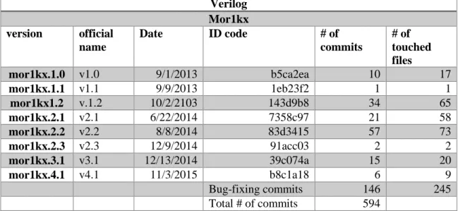
Mor1kx, the current design from the OpenRISC1000 processor family is the single package written in Verilog. Table 6 shows the existing released versions, the released date, the number of commits associated with each of them and the number of modified files before the next release.

Verilog Mor1kx version official name Date ID code # of commits # of touched files mor1kx.1.0 v1.0 9/1/2013 b5ca2ea 10 17 mor1kx.1.1 v1.1 9/9/2013 1eb23f2 1 1 mor1kx1.2 v.1.2 10/2/2103 143d9b8 34 65 mor1kx.2.1 v2.1 6/22/2014 7358c97 21 58 mor1kx.2.2 v2.2 8/8/2014 83d3415 57 73 mor1kx.2.3 v2.3 12/9/2014 91acc03 2 2 mor1kx.3.1 v3.1 12/13/2014 39c074a 15 20 mor1kx.4.1 v4.1 11/3/2015 b8c1a18 6 9 Bug-fixing commits 146 245 Total # of commits 594

Table 5: Released versions for Mor1kx project

(42)

Table 6: Mor1kx HCT metrics summary

4.4.2 The “C” Subprojects Group

The second analyzed subproject ORK-Sim written in C had also eight released versions. They are presented in Table 8.

By using the UnderstandSCI tool, we were able to compute the complexity metrics for each package and each version.

An example of some complexity metrics statistics for each Or1k-sim released version is presented in the next table.

C Or1k-sim

version official name date ID code # of

commits

# of touched files

or1ksim-0.3.0 or1ksim-0.3.0 5/25/2009 0b63f32 3 148

or1ksim-0.4.0rc1 or1ksim-0.4.0rc1 6/3/2010 48c3d23 12 130

or1ksim-0.4.0rc2 or1ksim-0.4.0rc2 6/16/2010 c7a1d5e 2 14

or1ksim-0.4.0 or1ksim-0.4.0 6/22/2010 27806aa 15 208

or1ksim-0.5.0rc1 or1ksim-0.5.0rc1 9/7/2010 ef54033 2 22

or1ksim-0.5.0rc2 or1ksim-0.5.0rc2 10/2/2010 b55e843 21 131

or1ksim-0.5.0rc3 or1ksim-0.5.0rc3 2/11/2011 ae337dc 2 50

or1ksim-0.5.1rc1 or1ksim-0.5.1rc1 4/8/2011 7672c7e 45 179

Bug-fixing commits 102 882

Total # of commits 129

Table 7: Released versions for Or1k-sim project

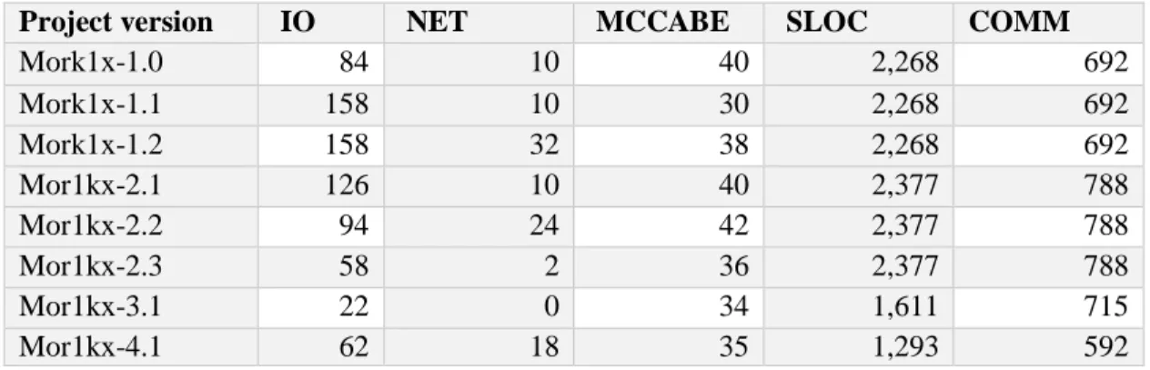
Project version IO NET MCCABE SLOC COMM

Mork1x-1.0 84 10 40 2,268 692 Mork1x-1.1 158 10 30 2,268 692 Mork1x-1.2 158 32 38 2,268 692 Mor1kx-2.1 126 10 40 2,377 788 Mor1kx-2.2 94 24 42 2,377 788 Mor1kx-2.3 58 2 36 2,377 788 Mor1kx-3.1 22 0 34 1,611 715 Mor1kx-4.1 62 18 35 1,293 592

(43)

We wanted to study the following two research questions regarding the defect prediction studies on the OpenRISC1000 hardware repository:

1. Classification: to predict the files which contain software bugs (e.g., Mor1kx or Or1k-sim) and,

2. Ranking: to predict the files which contain the largest number of software defects.

4.4.3 Classification

The first analysis that had to be done was naturally the classification. Using this method, we were able to differentiate between buggy or not buggy files. In this work, we compared the results built using the random forest and logistic regression model to see which prediction model provides the best results.

• Logistic regression is used to estimate the probability of a binary response based on one or more predictor variables. Logistic regression measures the relationship between the categorical dependent variable, in our case “buggy or not buggy” and one or more independent variables. To classify files/packages as defect-prone or not based on code metrics we define the following based on the values outputted by the logistic regression model:

Defect Classification =

defect-prone (0.5 < value ≤ 1) defect-free (0 ≤ value ≤ 0.5)

(44)

• Random forest is another useful prediction method when predicting a binary outcome [15], in our case post-release bugs from a set of continuous or categorical variables. Compared to the logistic regression model, in which there are a few assumptions associated with the model (e.g., the normality of the data, the balance of the output data, etc.), the random forest model is less constrained.

Since there were more “bug-free” files than the “buggy” files, we had to re-sample the data before we can train them using the logistic regression model. The data was sampled automatically before proceeding with the logistic regression method to every dataset. By doing this, we ensured that for every test dataset the number of buggy records equals the number of the not buggy ones. Every version from both projects was used as a training dataset and all the remaining versions became one after another the test dataset.

Below we describe the performance metrics used to evaluate the effectiveness of the defect prediction models: precision, recall, and F-measure.

To properly explain the above three metrics, we need to consider the following prediction outcomes (Table 9):

• True positive (TP): buggy instances predicted as buggy

• False positive (FP): clean instances predicted as buggy

• True negative (TN): clean instances predicted as clean

(45)

Actual Results

Yes No

Predictive Results Yes TP (true positive) FP (false positive) No FN (false negative) TN (true negative)

Table 8: Classification table

With these prediction outcomes, which are mostly used in the defect prediction literature, the following measures are defined:

• Precision – measures the ratio of the correctly classified positive modules to the set of positive modules.

• Recall – measures the ratio of correctly predicted positive modules in the whole modules with defects.

• F-measure – is the harmonic mean of precision and recall.

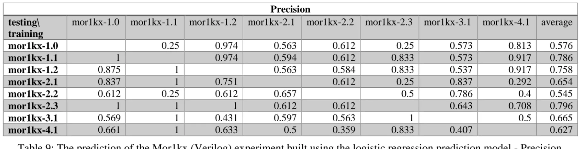
Having this knowledge and based on the output values, the data can be interpreted immediately and it is easy to know if a file or a package contains software defects or not. The Precision, Recall and F-measure values for the logistic regression models are listed below (Tables 10, 11, 12).

(46)

Precision testing\

training

mor1kx-1.0 mor1kx-1.1 mor1kx-1.2 mor1kx-2.1 mor1kx-2.2 mor1kx-2.3 mor1kx-3.1 mor1kx-4.1 average

mor1kx-1.0 0.25 0.974 0.563 0.612 0.25 0.573 0.813 0.576 mor1kx-1.1 1 0.974 0.594 0.612 0.833 0.573 0.917 0.786 mor1kx-1.2 0.875 1 0.563 0.584 0.833 0.537 0.917 0.758 mor1kx-2.1 0.837 1 0.751 0.612 0.25 0.837 0.292 0.654 mor1kx-2.2 0.612 0.25 0.612 0.657 0.5 0.786 0.4 0.545 mor1kx-2.3 1 1 1 0.612 0.612 0.643 0.708 0.796 mor1kx-3.1 0.569 1 0.431 0.597 0.563 1 0.5 0.665 mor1kx-4.1 0.661 1 0.633 0.5 0.359 0.833 0.407 0.627

Table 9: The prediction of the Mor1kx (Verilog) experiment built using the logistic regression prediction model - Precision

Recall testing\

training

mor1kx-1.0 0.5 0.972 0.563 0.611 0.5 0.571 0.7 0.631 mor1kx-1.1. 1 0.972 0.594 0.611 0.75 0.571 0.9 0.771 mor1kx-1.2 0.833 1 0.563 0.583 0.75 0.536 0.9 0.737 mor1kx-2.1 0.833 1 0.75 0.611 0.5 0.821 0.3 0.687 mor1kx-2.2 0.611 0.5 0.611 0.656 0.5 0.786 0.4 0.58 mor1kx-2.3 1 1 1 0.611 0.611 0.643 0.7 0.795 mor1kx-3.1 0.556 1 0.444 0.594 0.556 1 0.5 0.664 mor1kx-4.1 0.611 1 0.583 0.5 0.444 0.75 0.464 0.621

Table 10: The prediction of the Mor1kx (Verilog) experiment built using the logistic regression prediction model - Recall

(47)

testing\ training

mor1kx-1.0 0.333 0.972 0.563 0.61 0.333 0.569 0.67 0.578 mor1kx-1.1 1 0.972 0.593 0.61 0.733 0.569 0.899 0.768 mor1kx-1.2 0.829 1 0.561 0.583 0.733 0.53 0.899 0.733 mor1kx-2.1 0.833 1 0.75 0.61 0.333 0.819 0.293 0.662 mor1kx-2.2 0.61 0.333 0.61 0.656 0.5 0.786 0.4 0.556 mor1kx-2.3 1 1 1 0.61 0.61 0.643 0.697 0.794 mor1kx-3.1 0.532 1 0.416 0.59 0.543 1 0.495 0.653 mor1kx-4.1 0.579 1 0.54 0.382 0.345 0.733 0.367 0.536

(48)

The above charts show that the vast majority of the values for precision, recall, and accuracy are in the [0.5:1] interval. It means we can use the logistic regression method to perform bug prediction on all mor1kx versions.

Similarity, we used one version of the data as training data for the random forest model and tested it against other versions. The tables below show the precision, recall and F-measure number for the Mor1kx project obtained by using this second method (Tables 13, 14, 15 for Mor1kx ).

By analyzing the precision, recall, and accuracy results obtained through the random forest method, we can reach the same conclusion as for the logistic regression method: we can use the random forest method to perform bug prediction on all mor1kx versions. In addition, the prediction performance for the random forest method is better than the logistic regression method.

(49)

Precision testing\

training

mor1kx-1.0 1 1 0.65 0.594 0.974 0.644 0.946 0.829 mor1kx-1.1. 0.832 0.757 0.76 0.237 0.974 0.776 0.904 0.748 mor1kx-1.2 1 1 0.598 0.594 0.974 0.622 0.946 0.819 mor1kx-2.1 0.861 0.974 0.951 0.732 0.951 0.76 0.716 0.849 mor1kx-2.2 0.677 0.924 0.679 0.736 0.896 0.683 0.735 0.761 mor1kx-2.3 0.832 1 0.757 0.765 0.757 0.787 0.834 0.818 mor1kx-3.1 0.875 0.975 0.759 0.75 0.639 0.954 0.771 0.817 mor1kx-4.1 0.849 1 0.771 0.367 0.586 0.946 0.654 0.739

Table 12: The prediction of the Mor1kx (Verilog) experiment built using the random forest prediction model - Precision

Recall testing\

training

mor1kx-1.0 1 0.947 0.619 0.595 0.973 0.649 0.946 0.818 mor1kx-1.1 0.784 0.514 0.459 0.486 0.973 0.649 0.892 0.679 mor1kx-1.2 1 1 0.595 0.595 0.973 0.622 0.946 0.818 mor1kx-2.1 0.676 0.459 0.946 0.73 0.486 0.703 0.405 0.629 mor1kx-2.2 0.568 0.514 0.676 0.73 0.486 0.649 0.459 0.583 mor1kx-2.3 0.784 1 0.514 0.486 0.514 0.676 0.865 0.691 mor1kx-3.1 0.838 0.676 0.73 0.703 0.622 0.703 0.595 0.695 mor1kx-4.1 0.811 1 0.568 0.405 0.514 0.946 0.649 0.699

Table 13: The prediction of the Mor1kx (Verilog) experiment built using the random forest prediction model - Recall

(50)

testing\ training

mor1kx-1.0 1 0.973 0.634 0.594 0.969 0.646 0.946 0.823 mor1kx-1.1 0.711 0.376 0.318 0.318 0.969 0.535 0.859 0.583 mor1kx-1.2 1 1 0.596 0.594 0.969 0.622 0.946 0.818 mor1kx-2.1 0.696 0.601 0.946 0.729 0.603 0.706 0.489 0.681 mor1kx-2.2 0.598 0.66 0.675 0.731 0.612 0.654 0.541 0.638 mor1kx-2.3 0.711 1 0.376 0.37 0.376 0.588 0.839 0.608 mor1kx-3.1 0.846 0.782 0.724 0.7 0.613 0.784 0.657 0.729 mor1kx-4.1 0.761 1 0.477 0.289 0.411 0.946 0.569 0.636

(51)

Based on the existing data, we have plotted 3 graphs where logistic regression and random forest can be accurately compared (Figures 11, 12, 13).

Figure 11: Mor1kx – Precision

(52)

Figure 13: Mor1kx - F-Measure

We did a similar study for the Or1k-sim subproject. We applied both the logistic regression and the random forest methods. In this second study, the values for precision, recall, and accuracy were in the [0.92:0.99] interval. Similar as the mor1kx versions, the precision, recall, and F-measure values obtained through the random forest method were a little bit higher than the ones obtained through the logistic regression. The data is shown in the following tables.

(53)

Precision test\training or1k-sim.0.3.0 or1k-sim.0.4.0 or1k-sim.0.4.0.rc1 or1k-sim.0.4.0.rc2 or1k-sim.0.5.0.rc1 or1k-sim.0.5.0.rc2 or1k-sim.0.5.0.rc3 or1k-sim.0.5.1.rc1 average or1k-sim.0.3.0 0.97 0.978 1 0.978 0.957 0.987 0.953 0.974 or1k-sim.0.4.0 0.963 0.936 0.982 0.981 0.944 0.969 0.902 0.953 or1k-sim.0.4.0.rc1 0.948 0.922 0.979 0.96 0.906 0.94 0.922 0.939 or1k-sim.0.4.0.rc2 0.943 0.912 0.95 0.921 0.922 0.93 0.887 0.923 or1k-sim.0.5.0.rc1 0.959 0.942 0.958 0.965 0.937 0.974 0.93 0.952 or1k-sim.0.5.0.rc2 0.979 0.983 0.967 0.991 0.991 0.982 0.966 0.979 or1k-sim.0.5.0.rc3 0.979 0.959 0.962 0.996 0.987 0.974 0.953 0.972 or1k-sim.0.5.1.rc1 1 0.987 0.986 1 0.991 0.987 1 0.993

Table 15: The prediction of the Or1k-sim (C) experiment built using the logistic regression prediction model - Precision

Recall test\training or1k-sim.0.3.0 or1k-sim.0.4.0 or1k-sim.0.4.0.rc1 or1k-sim.0.4.0.rc2 or1k-sim.0.5.0.rc1 or1k-sim.0.5.0.rc2 or1k-sim.0.5.0.rc3 or1k-sim.0.5.1.rc1 average

(54)

or1k-sim.0.3.0 0.969 0.978 1 0.978 0.955 0.987 0.951 0.974 or1k-sim.0.4.0 0.961 0.947 0.982 0.982 0.946 0.973 0.901 0.956 or1k-sim.0.4.0.rc1 0.952 0.929 0.973 0.964 0.919 0.951 0.915 0.943 or1k-sim.0.4.0.rc2 0.939 0.902 0.947 0.96 0.915 0.964 0.87 0.928 or1k-sim.0.5.0.rc1 0.957 0.938 0.956 0.982 0.933 0.973 0.924 0.951 or1k-sim.0.5.0.rc2 0.978 0.982 0.969 0.991 0.991 0.982 0.964 0.979 or1k-sim.0.5.0.rc3 0.978 0.96 0.964 0.996 0.987 0.973 0.951 0.972 or1k-sim.0.5.1.rc1 1 0.987 0.987 1 0.991 0.987 1 0.993

Table 16: The prediction of the Or1k-sim (C) experiment built using the logistic regression prediction model - Recall

F-Measure test\training or1k-sim.0.3.0 or1k-sim.0.4.0 or1k-sim.0.4.0.rc1 or1k-sim.0.4.0.rc2 or1k-sim.0.5.0.rc1 or1k-sim.0.5.0.rc2 or1k-sim.0.5.0.rc3 or1k-sim.0.5.1.rc1 average or1k-sim.0.3.0 0.966 0.975 1 0.973 0.949 0.985 0.946 0.97 or1k- 0.953 0.936 0.982 0.981 0.938 0.969 0.88 0.948

(55)

F-Measure test\training or1k-sim.0.3.0 or1k-sim.0.4.0 or1k-sim.0.4.0.rc1 or1k-sim.0.4.0.rc2 or1k-sim.0.5.0.rc1 or1k-sim.0.5.0.rc2 or1k-sim.0.5.0.rc3 or1k-sim.0.5.1.rc1 average sim.0.4.0 or1k-sim.0.4.0.rc1 0.95 0.922 0.976 0.962 0.908 0.945 0.898 0.937 or1k-sim.0.4.0.rc2 0.914 0.863 0.927 0.94 0.882 0.947 0.817 0.898 or1k-sim.0.5.0.rc1 0.946 0.926 0.944 0.973 0.915 0.965 0.911 0.94 or1k-sim.0.5.0.rc2 0.976 0.982 0.966 0.991 0.991 0.982 0.962 0.978 or1k-sim.0.5.0.rc3 0.976 0.957 0.96 0.995 0.985 0.971 0.946 0.97 or1k-sim.0.5.1.rc1 1 0.987 0.986 1 0.99 0.986 1 0.992

Table 17: The prediction of the Or1k-sim (C) experiment built using the logistic regression prediction model - F-Measure

Random forest method

(56)

test\training or1k-sim.0.3.0 or1k-sim.0.4.0 or1k-sim.0.4.0.rc1 or1k-sim.0.4.0.rc2 or1k-sim.0.5.0.rc1 or1k-sim.0.5.0.rc2 or1k-sim.0.5.0.rc3 or1k-sim.0.5.1.rc1 average or1k-sim.0.3.0 0.97 0.978 1 0.978 0.957 0.987 0.953 0.974 or1k-sim.0.4.0 0.963 0.936 0.982 0.981 0.944 0.969 0.902 0.953 or1k-sim.0.4.0.rc1 0.948 0.922 0.979 0.96 0.906 0.94 0.922 0.939 or1k-sim.0.4.0.rc2 0.943 0.912 0.95 0.921 0.922 0.93 0.887 0.923 or1k-sim.0.5.0.rc1 0.959 0.942 0.958 0.965 0.937 0.974 0.93 0.952 or1k-sim.0.5.0.rc2 0.979 0.983 0.967 0.991 0.991 0.982 0.966 0.979 or1k-sim.0.5.0.rc3 0.979 0.959 0.962 0.996 0.987 0.974 0.953 0.972 or1k-sim.0.5.1.rc1 1 0.987 0.986 1 0.991 0.987 1 0.993

Table 18: The prediction of the Or1k-sim (C) experiment built using the random forest prediction model - Precision

Recall test\training or1k-sim.0.3.0 or1k-sim.0.4.0 or1k-sim.0.4.0.rc1 or1k-sim.0.4.0.rc2 or1k-sim.0.5.0.rc1 or1k-sim.0.5.0.rc2 or1k-sim.0.5.0.rc3 or1k-sim.0.5.1.rc1 average or1k-sim.0.3.0 0.969 0.978 1 0.978 0.955 0.987 0.951 0.974

(57)

Recall test\training or1k-sim.0.3.0 or1k-sim.0.4.0 or1k-sim.0.4.0.rc1 or1k-sim.0.4.0.rc2 or1k-sim.0.5.0.rc1 or1k-sim.0.5.0.rc2 or1k-sim.0.5.0.rc3 or1k-sim.0.5.1.rc1 average or1k-sim.0.4.0 0.961 0.947 0.982 0.982 0.946 0.973 0.901 0.956 or1k-sim.0.4.0.rc1 0.952 0.929 0.973 0.964 0.919 0.951 0.915 0.943 or1k-sim.0.4.0.rc2 0.939 0.902 0.947 0.96 0.915 0.964 0.87 0.928 or1k-sim.0.5.0.rc1 0.957 0.938 0.956 0.982 0.933 0.973 0.924 0.951 or1k-sim.0.5.0.rc2 0.978 0.982 0.969 0.991 0.991 0.982 0.964 0.979 or1k-sim.0.5.0.rc3 0.978 0.96 0.964 0.996 0.987 0.973 0.951 0.972 or1k-sim.0.5.1.rc1 1 0.987 0.987 1 0.991 0.987 1 0.993

Table 19: The prediction of the Or1k-sim (C) experiment built using the random forest prediction model - Recall

F-Measure test\training or1k-sim.0.3.0 or1k-sim.0.4.0 or1k-sim.0.4.0.rc1 or1k-sim.0.4.0.rc2 or1k-sim.0.5.0.rc1 or1k-sim.0.5.0.rc2 or1k-sim.0.5.0.rc3 or1k-sim.0.5.1.rc1 average

(58)

or1k-sim.0.3.0 0.966 0.975 1 0.973 0.949 0.985 0.946 0.97 or1k-sim.0.4.0 0.953 0.936 0.982 0.981 0.938 0.969 0.88 0.948 or1k-sim.0.4.0.rc1 0.95 0.922 0.976 0.962 0.908 0.945 0.898 0.937 or1k-sim.0.4.0.rc2 0.914 0.863 0.927 0.94 0.882 0.947 0.817 0.898 or1k-sim.0.5.0.rc1 0.946 0.926 0.944 0.973 0.915 0.965 0.911 0.94 or1k-sim.0.5.0.rc2 0.976 0.982 0.966 0.991 0.991 0.982 0.962 0.978 or1k-sim.0.5.0.rc3 0.976 0.957 0.96 0.995 0.985 0.971 0.946 0.97 or1k-sim.0.5.1.rc1 1 0.987 0.986 1 0.99 0.986 1 0.992

(59)

Similar graphs were plotted to compare the logistical regression and random forest methods, for Or1k-sim project in this case (Figures 14, 15, 16).

Figure 14: Or1k-sim- Precision

(60)

Figure 16: Or1k-sim F-Measure

Using classification through logistic regression, we were able to determine which released versions were prone to software defects. The data indicated that the Mor1kx.1.1 and Or1k-sim.0.4.0.rc2 were the most prone to bugs versions.

In general, the random forest models had higher precision than the logistic regression models for both Or1k and Mor1kx sub-projects. For the Or1k sub-project, the random forest model generally out-performed the logistic regression model in all three metrics (precision, recall, and F-measure).

4.4.4 Ranking

To answer the second question related to which files and released versions contain the most of the software defects, we applied the linear regression method and the entropy method to the “number of bugs field” for every remaining version of those 2 projects.

(61)

• Given a dataset of n statistical units, a linear

regression model assumes that the relationship between the dependent variable yi and the p-vector of regressors xi is linear.

Another idea to predict the number of bugs is based on the entropy of changes.

Hassan et al proposed the use of Shannon Entropy defined as [2]: . The idea consists in measuring over a time interval how the changes are distributed in a system. The more spread they are, the higher the complexity is.

To evaluate the effectiveness of the above two ranking approaches, we used the Spearman correlation coefficient as a statistical tool to measure the strength of the relationship between two sets of data. The values of Spearman’s correlation coefficient can be between -1 and +1. A positive correlation coefficient indicates a positive relationship between the two variables (the higher the x values, also the higher the y values), while a negative correlation coefficient expresses a negative relationship (the lower the x values, the lower the y values). A correlation coefficient of 0 indicates that there is no relationship between the two studied variables.

In our case, the Spearman’s correlation coefficient measures the correlation between the predicted bugs and the existing observed bugs. The results are shown in Tables 22 and 23.

(62)

Spearman Correlation Coefficient

testing\training mor1kx-1.0 mor1kx-1.1 mor1kx-1.2 mor1kx-2.1 mor1kx-2.2 mor1kx-2.3 mor1kx-3.1 mor1kx-4.1 average

mor1kx-1.0 0.2035 0.8824 0.584 0.6509 0.2164 0.4369 0.2301 0.457 mor1kx-1.1. 0.8356 0.9541 0.9724 0.9513 0.9227 0.8743 0.955 0.923 mor1kx-1.2 0.7179 0.0116 0.3585 0.0978 0.0111 0.1542 0.0362 0.198 mor1kx-2.1 0.0551 0.0202 0.4266 0.1241 0.0207 0.0724 0.1166 0.119 mor1kx-2.2 0.0107 0.1244 0.0906 0.0188 0.1238 0.5347 0.0311 0.133 mor1kx-2.3 0.4444 0.9964 0.6525 0.5799 0.6065 0.3685 0.5129 0.594 mor1kx-3.1 0.4852 0.1868 0.7065 0.5914 0.8507 0.1817 0.1883 0.455 mor1kx-4.1 0.4981 0.3755 0.8581 0.8544 0.8623 0.372 0.462 0.611

Table 21: Mor1kx – Spearman correlation coefficient

Spearman Correlation Coefficient test\ training or1k-sim.0.3.0 or1k-sim.0.4.0 or1k-sim.0.4.0.rc1 or1k-sim.0.4.0.rc2 or1k-sim.0.5.0.rc1 or1k-sim.0.5.0.rc2 or1k-sim.0.5.0.rc3 or1k-sim.0.5.1.rc1 average