repository: http://orca.cf.ac.uk/124466/
This is the author’s version of a work that was submitted to / accepted for publication.
Citation for final published version:
Grahovac, Danijel, Leonenko, Nikolai N. and Taqqu, Murad S. 2020. The multifaceted behavior of
integrated supOU processes: The infinite variance case. Journal of Theoretical Probability 33 , pp.
1801-1831. 10.1007/s10959-019-00935-8 file
Publishers page: https://doi.org/10.1007/s10959-019-00935-8
<https://doi.org/10.1007/s10959-019-00935-8>
Please note:
Changes made as a result of publishing processes such as copy-editing, formatting and page
numbers may not be reflected in this version. For the definitive version of this publication, please
refer to the published source. You are advised to consult the publisher’s version if you wish to cite
this paper.
This version is being made available in accordance with publisher policies. See
http://orca.cf.ac.uk/policies.html for usage policies. Copyright and moral rights for publications
made available in ORCA are retained by the copyright holders.
(will be inserted by the editor)
The multifaceted behavior of integrated supOU
processes: The infinite variance case
Danijel Grahovac · Nikolai N. Leonenko ·
Murad S. Taqqu
Received: date / Accepted: date
Abstract The so-called “supOU” processes, namely the superpositions of Ornstein-Uhlenbeck type processes are stationary processes for which one can specify separately the marginal distribution and the temporal dependence structure. They can have finite or infinite variance. We study the limit be-havior of integrated infinite variance supOU processes adequately normalized. Depending on the specific circumstances, the limit can be fractional Brownian motion but it can also be a process with infinite variance, a L´evy stable process with independent increments or a stable process with dependent increments. We show that it is even possible to have infinite variance integrated supOU processes converging to processes whose moments are all finite. A number of examples are provided.
Keywords supOU processes·Ornstein-Uhlenbeck process·limit theorems·
infinite variance·stable processes
Mathematics Subject Classification (2010) 60F05· 60G52·60G10 1 Introduction
SupOU processes which are defined below are superpositions of stationary Ornstein-Uhlenbeck processes driven by a L´evy process. They were
stud-D. Grahovac
Department of Mathematics, University of Osijek, 31000 Osijek, Croatia Tel.: +385-31-224800
Fax: +385-31-224801 E-mail: [email protected] N. N. Leonenko
Cardiff School of Mathematics, Cardiff University, Cardiff, CF24 4AG, UK E-mail: [email protected]
M. S. Taqqu
Department of Mathematics and Statistics, Boston University, Boston, MA 02215, USA E-mail: [email protected]
ied extensively by Barndorff-Nielsen and his collaborators Barndorff-Nielsen (2001), Barndorff-Nielsen & Stelzer (2011), Barndorff-Nielsen & Stelzer (2013), Barndorff-Nielsen & Veraart (2013). An attractive feature of supOU processes is that they allow the marginal distribution and the temporal dependence structure to be modeled independently.
ThesupOU process is defined as follows: it is a strictly stationary process
X ={X(t), t∈R} represented by the stochastic integral (Barndorff-Nielsen (2001)) X(t) = Z R+ Z R e−ξt+s1[0,∞)(ξt−s)Λ(dξ, ds). (1)
Here,Λis a homogeneous infinitely divisible random measure (L´evy basis) on R+×R, with cumulant function forA∈ B(R+×R)
C{ζ‡Λ(A)}:= logEeiζΛ(A)=m(A)κL(ζ) = (π×Leb) (A)κL(ζ). (2) The control measure m = π×Leb is the product of a probability measure
π on R+ and the Lebesgue measure on R. The probability measure π “ran-domizes” the rate parameter ξ and the Lebesgue measure is associated with the moving average variable s. Finally, κL in (2) is the cumulant function κL(ζ) = logEeiζL(1) of some infinitely divisible random variable L(1) with L´evy-Khintchine triplet (a, b, µ) i.e.
κL(ζ) =iζa−ζ 2 2b+ Z R eiζx−1−iζx1[−1,1](x) µ(dx). (3) The L´evy process L = {L(t), t ≥ 0} associated with the triplet (a, b, µ) is called thebackground driving L´evy process and the quadruple
(a, b, µ, π) (4)
is referred to as thecharacteristic quadruple.
The marginal distribution of X is determined byL, while the dependence structure is controlled by the probability measureπ. Indeed, if EX(t)2 <∞, then the correlation function ofX is the Laplace transform ofπ:
r(t) = Z
R+
e−tξπ(dξ), t≥0. (5) More details about supOU processes can be found in Barndorff-Nielsen (2001), Nielsen & Leonenko (2005), Nielsen et al. (2013), Barndorff-Nielsen & Stelzer (2011) and Grahovac, Leonenko, Sikorskii & Taqqu (2019).
Integrated supOU processX∗={X∗(t), t≥0} defined by
X∗(t) = Z t
0
X(s)ds, (6)
has a complex asymptotic behavior. We have shown in Grahovac, Leonenko & Taqqu (2019) that when the supOU process has a finite variance, then different types of limits of integrated process can occur depending on the
specific structure of the process. In this paper, we study what happens when the supOU has infinite variance. We show that again different limits can occur depending in particular on how heavy the tails of the supOU process are. We show that it is possible to have an infinite variance process to converge to a process with all moments finite.
Our results may be of particular interest in financial econometrics where supOU processes are used as stochastic volatility models and hence the in-tegrated process X∗ represents the integrated volatility (see e.g.
Barndorff-Nielsen & Stelzer (2013)). The limiting behavior is also important for statisti-cal estimation (see Stelzer et al. (2015), Curato & Stelzer (2019)). In Grahovac, Leonenko & Taqqu (2019) it has been shown that integrated supOU processes may exhibit an interesting phenomenon of intermittency which may be rele-vant for applications in turbulence (see e.g. Zel’dovich et al. (1987)).
When the supOU process{X(t), t∈R} has finite variance, four different limiting processes may be obtained depending on the elements of the charac-teristic quadruple, namely
– Brownian motion,
– fractional Brownian motion, – a stable L´evy process,
– a stable process with dependent increments defined in (18) below.
The type of limit depends on whether Gaussian component is present in (4), on a parameterαquantifying dependence and on a parameter β quantifying the growth of the L´evy measureµin (4) near origin.
We show in this paper that when the supOU process {X(t), t∈ R} has infinite variance, the limiting behavior depends additionally on the regular variation index γ of the marginal distribution. As limiting process, one can obtain
– a stable L´evy process,
– a stable process with dependent increments defined in (18) below, – fractional Brownian motion.
We provide examples to illustrate the results.
The paper is organized as follows. In Section 2 we list the assumptions used for our results. Section 3 contains the main results and in Section 4 examples are provided. All the proofs are contained in Section 5.
2 Basic assumptions
Before stating the main results we introduce some notation and basic assump-tions.
2.1 Preliminaries
A random variable Z with an infinite variance stable distribution Sγ(σ, ρ, c) and parameters 0 < γ < 2, σ >0, −1 ≤ ρ ≤1 and c ∈ R has a cumulant
function of the form κSγ(σ,ρ,c)(ζ) :=C{ζ‡Z}=icζ−σ γ|ζ|γ(1−iρsign(ζ)χ(ζ, γ)), ζ∈R, (7) where χ(ζ, γ) = ( tan πγ2 , γ6= 1, π 2log|ζ|, γ= 1.
For simplicity of the exposition, wherever it applies we will assumeZ is sym-metric (ρ= 0) whenγ= 1, hence we can write
χ(ζ, γ) =χ(γ) = (
tan πγ2 , γ6= 1,
0, γ= 1.
We shall make a number of basic assumptions.
2.2 Domain of attraction
We suppose that the marginal distribution of the supOU process{X(t), t∈R}
in (1) belongs to the domain of attraction of stable law, that is, X(1) has balanced regularly varying tails:
P(X(1)> x)∼pk(x)x−γ and P(X(1)≤ −x)∼qk(x)x−γ, asx→ ∞,
(8) for somep, q ≥0,p+q >0, 0< γ <2 and some slowly varying function k. If γ = 1, we assume p=q. In particular, the variance is infinite. Moreover, when the mean is finite, that is when γ > 1, we assume EX(1) = 0. These assumptions imply thatX(1) is in the domain of attraction ofSγ(σ, ρ,0) law with (Ibragimov & Linnik 1971, Theorem 2.6.1)
σ= Γ(2−γ) 1−γ (p+q) cos πγ 2 1/γ , ρ=p−q p+q. (9)
Now consider the L´evy process{L(t), t≥0}introduced in Section 1. By (Fasen & Kl¨uppelberg 2007, Propositon 3.1), the tail of the distribution function of
X(1) is asymptotically equivalent to the tail of the background driving L´evy processL(t) at t= 1. More precisely, as x→ ∞
P(L(1)> x)∼γP(X(1)> x) and P(L(1)≤ −x)∼γP(X(1)≤ −x).
(10) Hence, (8) implies
P(L(1)> x)∼pγk(x)x−γ and P(L(1)≤ −x)∼qγk(x)x−γ, as x→ ∞,
(11) andL(1) is in the domain of attraction of stable distributionSγ(γ1/γσ, ρ,0). Note that the scale parameter σ of X(1) yields a scale parameter γ1/γσ for L(1).
The normalizing sequence in some of the limit theorems below involves the de Bruijn conjugate of a slowly varying function (Bingham et al. 1989, Subsection 1.5.7). Recall that the de Bruijn conjugate of some slowly varying functionhis a slowly varying functionh#such that
h(x)h#(xh(x))→1, h#(x)h(xh#(x))→1,
as x → ∞. By (Bingham et al. 1989, Theorem 1.5.13) such function always exists and is unique up to asymptotic equivalence.
2.3 Dependence structure
The second set of assumptions deals with the temporal dependence structure dictated by the behavior near the origin of the probability measure πin the characteristic quadruple (4). We will assume that the probability measure π
is regularly varying at zero, that is for some α >0 and some slowly varying functionℓ
π((0, x])∼ℓ(x−1)xα, asx→0. (12) To simplify the proofs of some of the results below, we will assume thatπhas a densitypwhich is monotone on (0, x′) for somex′ >0, so that (12) implies
p(x)∼αℓ(x−1)xα−1, asx→0. (13) To see how this affects dependence, note that if the variance is finiteEX(t)2<
∞, then (5) and (12) imply that the correlation function satisfies (Fasen & Kl¨uppelberg 2007, Proposition 2.6)
r(τ)∼Γ(1 +α)ℓ(τ)τ−α, asτ→ ∞.
Hence, if α∈(0,1), the correlation function is not integrable, and the finite variance supOU process may be said to exhibit long-range dependence. On the other hand, note that the behavior ofπ at infinity does not affect the decay of correlations as decay of correlations depends on the asymptotics of πnear zero. To simplify the presentation of the results, we shall assume that
Z ∞
0
ξπ(dξ)<∞. (14)
2.4 Behavior of the L´evy measure at the origin
Unlike classical limit theorems, the limiting distribution of the integrated supOU processes does not depend only on the tails of the marginal distri-bution and on the dependence structure. The third component affecting the limit is the growth of the L´evy measure µ near origin. We will quantify this
growth by assuming a power law behavior of the L´evy measure near the origin. Let
M+(x) =µ([x,∞)), x >0, M−(x) =µ((−∞,−x]), x >0,
denote the tails of µ. We will assume that there exists β ≥ 0, c+, c− ≥ 0,
c++c−>0 such that
M+(x)∼c+x−β and M−(x)∼c−x−β as x→0. (15) Sinceµis the L´evy measure, we must haveβ <2. If (15) holds, thenβ is the Blumenthal-Getoor index of the L´evy measure µ defined by (see Grahovac, Leonenko & Taqqu (2019))
βBG= inf ( γ≥0 : Z |x|≤1| x|γµ(dx)<∞ ) . (16)
Note that by (Kyprianou 2014, Lemma 7.15) M+(x) ∼ P(L(1) > x) and
M−(x)∼P(L(1)≤ −x) asx→ ∞, hence we can express (11) equivalently as
M+(x)∼pγk(x)x−γ and M−(x)∼qγk(x)x−γ, as x→ ∞.
In general, making assumptions on the value of the Blumenthal-Getoor index
βBGis more general than assuming (15). For example, in the geometric stable example in Subsection 4.4 below, the mass of the L´evy measure near the origin increases at the logarithmic rate, hence (15) does not hold but βBG = 0. Certain parts of our main results below require only assumptions on the value of the Blumenthal-Getoor index and not (15) (see Remark 1).
The condition (15) may be equivalently stated in terms of the L´evy measure ofX(1). Indeed, ifν is the L´evy measure ofX(1), then (15) is equivalent to
ν([x,∞))∼β−1c+x−β and ν((−∞,−x])∼β−1c−x−β as x→0. (17) See Grahovac, Leonenko & Taqqu (2019) for details.
3 Main results
Before stating the main theorems, let us review the parameters introduced in the previous section:
– γ ∈ (0,2) defined in (8) is the regular variation index of the marginal distribution,
– α∈(0,∞) defined in (13) quantifies the strength of dependence,
– β ∈[0,2) defined in (15) is the power law exponent of the L´evy measureµ
The resulting limiting process depends on the interplay between the parame-tersα,βandγ. In the next theorem, the process{X(t), t∈R}has no Gaussian component. Here and in what follows, {·}f dd→ {·} denotes the convergence of finite dimensional distributions.
Theorem 1 Suppose that the supOU process {X(t), t∈R} is such that – b= 0, thus has no Gaussian component,
– the marginal distribution satisfies (8)with 0< γ <2,
– the behavior at the origin of the L´evy measure µ is given by (15) with 0≤β <2,
– π has a density p satisfying (13) with α > 0 and some slowly varying function ℓ and (14)holds.
Then the following holds:
(I) Ifγ <1 +α, then asT → ∞
1
T1/γk#(T)1/γX
∗(T t)f dd→ {L
γ(t)},
where kis the slowly varying function in (8),k# is the de Bruijn con-jugate of1/k x1/γand the limit {L
γ} is aγ-stable L´evy process such that Lγ(1) d =Sγ(σe1,γ, ρ,0) with e σ1,γ=σ γ Z ∞ 0 ξ1−γπ(dξ) 1/γ ,
andσ andρgiven by (9).
(II) Ifγ >1 +α, then the limit depends on the value ofβ, as follows. (II.a) Ifβ <1 +α, then asT → ∞ ( 1 T1/(1+α)ℓ#(T)1/(1+α)X ∗(T t) ) f dd → {L1+α(t)},
where the limit{L1+α}is a (1 +α)-stable L´evy process such that L1+α(1)=d S1+α(σ,e ρ,e0) with e σ=σe1+1,βα+σe21+,αα1/(1+α), ρe=ρe1,βσe 1+α 1,β +ρe2,αeσ1+2,αα e σ11+,βα+eσ21+,αα ,
witheσ1,β andρe1,β defined in Lemma 2 andeσ2,α andρe2,α defined in Lemma 4 below. (II.b) If 1 +α < β, then asT → ∞ 1 T1−α/βℓ(T)1/βX ∗(T t) f dd → {Zα,β(t)},
where{Zα,β} is a process with the stochastic integral representa-tion Zα,β(t) = Z R+ Z R (f(ξ, t−s)−f(ξ,−s))K(dξ, ds), (18) fis given by f(x, u) = ( 1−e−xu, if x >0 andu >0, 0, otherwise, (19)
andK is aβ-stable L´evy basis onR+×Rwith control measure
αξαdξdssuch that C{ζ‡K(A)}=κ Sβ(σe2,β,ρe2,β,0)(ζ) with e σ2,β = Γ(2−β) 1−β (c −+c+) cos πβ 2 1/β , ρe2,β= c−−c+ c−+c+, and c−, c+ as in (15). The limit process {Z
α,β} has stationary increments and is self-similar with indexH= 1−α/β∈(1/β,1). Remark 1 We note that for the proof of Theorem 1(I) whenγ <1 one could replace (14) with the assumption that there existsε >0 such that
Z ∞
0
ξ1−γ+επ(dξ)<∞.
Also, for the proof of Theorem 1(II.a) instead of assuming (15) withβ <1+α, it is enough to assume that the Blumenthal-Getoor index (16) satisfiesβBG< 1 +α.
The first boundary between different limit types in Theorem 1 is given by
γ = 1 +α. By choosing formally γ = 2, we obtain α= 1 which corresponds to the boundary between short-range and long-range dependence in the finite variance case (see Grahovac, Leonenko & Taqqu (2019)).
In the infinite variance case, the regular variation indexγ of the marginal tails seems to play an important role in the limit only when γ <1 +α. One could say that in this scenariothe tails dominate the dependence structure. In the opposite case γ > 1 +α, two classes of stable processes may arise as a limit, either with dependent or independent increments. This depends on the value of parameterβ.
Note also that ifβ <1 +α < γ, the limiting processL1+αhas heavier tails than the supOU process whose tails are characterized byγ. On the other hand, when 1 +α < γ and 1 +α < β the limiting process has β-stable marginals hence, depending on whether β > γ or β < γ, the tails of the limit can be lighter or heavier than the tails of the underlying supOU process.
We now consider the case when the Gaussian component is present in the characteristic quadruple, that is b 6= 0. This is the main difference between Theorem 1 and Theorem 2.
Theorem 2 Suppose that the supOU process {X(t), t∈R} is such that – b6= 0, thus has a Gaussian component,
– the marginal distribution satisfies (8)with 0< γ <2,
– the behavior at the origin of the L´evy measure µ is given by (15) with 0≤β <2,
– π has a density p satisfying (13) with α > 0 and some slowly varying function ℓ and (14)holds.
(I) Ifα >1or if α <1 andγ < 2−2α, then asT → ∞
1
T1/γk#(T)1/γX∗(T t)
f dd
→ {Lγ(t)},
where the limit {Lγ} is a γ-stable L´evy process defined as in Theorem 1(I). (II) Ifα <1andγ > 2 2−α, then asT → ∞ 1 T1−α/2ℓ(T)1/2X ∗(T t)f dd→ {σe 3,αBH(t)},
where{BH(t)}is standard fractional Brownian motion withH = 1−α/2 andσe3,α=b2/2(2−Γα(1+)(1α−)α).
When the Gaussian component is present in the characteristic quadruple, the parameter β is irrelevant for the type of the limit process and there are only two possible limits. One is the L´evy stable motion {Lγ(t), t≥ 0} that would have been a limit if{X∗(t), t ≥0} had independent increments. The
second is the Gaussian fractional Brownian motion. In the first case, the limit has independent but infinite variance increments and in the second case the limit has dependent increments but their distribution is Gaussian.
Theorem 2 also provides an example of a limit theorem where the ag-gregated process has infinite variance, but the limiting process is fractional Brownian motion which has all the moments finite.
Figures 1 and 2 illustrate the limiting behavior graphically.
4 Examples
In this section we list several examples of supOU process and show how The-orems 1 and 2 apply. In each example we will fix the distribution of the back-ground driving L´evy process whileπmay be any absolutely continuous prob-ability measure satisfying (13). For example, π can be Gamma distribution with density f(x) = 1 Γ(α)x α−1e−x1 (0,∞)(x), whereα >0. Then π((0, x])∼ 1 Γ(α+ 1)x α, asx→0.
Fig. 1 Classification of limits ofX∗whenb= 0 stable L´evy processLγ 0 1 1 2 α γ
fractional Brownian motion
Fig. 2 Classification of limits ofX∗whenb6= 0
Other examples can be found in Grahovac, Leonenko, Sikorskii & Taqqu (2019).
In each of the examples bellow, we choose a background driving L´evy process such thatL(1) is a heavy-tailed distribution satisfying (11) with 0< γ <2 and (15) holds or the Blumenthal-Getoor index (16) is known.
Note that by appropriately choosing the background driving L´evy process
L, one can obtain any self-decomposable distribution as a marginal distribution ofX. Recall that an infinitely divisible random variableX isselfdecomposable if its characteristic function φ(θ) = EeiθX, θ ∈ R, has the property that for everyc ∈(0,1) there exists a characteristic functionφc such thatφ(θ) = φ(cθ)φc(θ) for allθ∈R(see e.g. Sato (1999)). Equivalently, for everyc∈(0,1) there is a random variable Yc such that the random variableX has the same distribution ascX+Yc.
Each of distributions given in examples below may be imposed as a dis-tribution of X(t). Indeed, every distribution considered in the following ex-amples is self-decomposable (see references cited below), hence there exists a background driving L´evy process generating a supOU process with such marginal distribution. Furthermore, if (8) holds, then L(1) satisfies (11) by (10). If (17) holds for the L´evy measure of X(1), then this implies (15) for the L´evy measure of L(1). Hence, Theorems 1 and 2 may still be applied as the conditions on the background driving L´evy process are easily translated to the corresponding conditions on the marginals of the supOU process.
4.1 Compound Poisson background driving L´evy process
Let L be a compound Poisson process with rate λ >0 and infinite variance jump distributionF regularly varying at infinity. More precisely,F satisfies
F((x,∞))∼pγk(x)x−γ and F((−∞,−x])∼qγk(x)x−γ, asx→ ∞,
for some 0< γ <2 andkslowly varying at infinity. IfF has a finite mean, then we assume it is zero. SupposeX is a supOU process with the background driv-ing L´evy processLandπabsolutely continuous probability measure satisfying (13). The characteristic quadruple (4) is then (a,0, µ, π) where
a=λ
Z
|x|≤1
xF(dx), µ(dx) =λF(dx).
Since the L´evy measure is finite, this case corresponds toβ = 0 in (15). Hence, Theorem 1 applies to show that the limit is stable L´evy process with indexγ
ifγ <1 +αor with index 1 +αifγ >1 +α.
4.2 Stable background driving L´evy process
Let L be aγ-stable L´evy process generating supOU processX with charac-teristic quadruple (4) given by (a,0, µ, π) where
µ(dx) = (
c1x−γ−1dx, x∈(0,∞),
with c1, c2 ≥ 0, c1+c2 > 0 if γ 6= 1 and c1 = c2 if γ = 1. If α > 1, we additionally assumeEX(1) = 0. The L´evy measure satisfies (15) withβ =γ
and from Theorem 1 we conclude that ifγ <1 +α, the limit isγ-stable L´evy process and if γ > 1 +α, then the limit is stable process Zα,γ defined in Theorem 1 (II.b). This type of limiting behavior was obtained by Puplinskait˙e & Surgailis (2010) for aggregated AR(1) processes with stable marginals.
4.3 Student’s background driving L´evy process
LetLbe a L´evy process such that L(1) has Student’st-distribution given by the density f(x) = Γ γ+1 2 δΓ 12Γ γ2 1 + x −c δ 2!−γ+1 2 , x∈R,
where c∈Ris location parameter, δ >0 scale parameter and the degrees of freedom 0< γ <2 correspond to the tail index of the distribution ofL(1) as in (11). Ifγ >1, we assumec= 0, henceEL(1) = 0. The L´evy-Khintchine triplet in (3) is (c,0, µ) with L´evy measureµabsolutely continuous with density
g(x) = 1 |x| Z ∞ 0 e−|x|√2y π2y(J2 γ/2(δ √ 2y) +Y2 γ/2(δ √ 2y))dy,
where Jγ/2 and Yγ/2 denote the Bessel functions of the first and the second kind, respectively (see e.g. Heyde & Leonenko (2005)). By (Eberlein & Ham-merstein 2004, Eq. (7.14)) we have
g(x)∼πδx−2, as x→0,
and by using Karamata’s theorem (Bingham et al. 1989, Theorem 1.5.11) it follows that
µ([x,∞))∼µ((−∞,−x])∼πδx−1, as x→0.
Hence,β = 1 in (15). Letπbe an absolutely continuous probability measure satisfying (13). Then the characteristic quadruple (4) is (c,0, µ, π). By The-orem 1 the limits are as in the compound Poisson case, namely, stable L´evy process with indexγ ifγ <1 +αor with index 1 +αifγ >1 +α.
4.4 Geometric stable background driving L´evy process
A random variable Y has a geometric stable distribution if its characteristic function has the form
EeiζY = 1 1−κSγ(σ,ρ,c)(ζ)
whereκSγ(σ,ρ,c)is the cumulant function (7) of some stable distributionSγ(σ, ρ, c).
The caseρ=c= 0 yields the so-called Linnik distribution with characteristic function (Bakeerathan & Leonenko (2008), Kotz et al. (2001))
EeiζY = 1
1 +σγ|ζ|γ, ζ∈R.
On the other hand, geometric stable distribution with 0 < γ < 1, σ = cos(πγ/2)1/γ, ρ = 1 and c = 0 is known as the Mittag-Leffler distribution (see Kozubowski (2001)).
LetLbe a L´evy process such thatL(1) has geometric stable distribution. For 0 < γ < 2, geometric stable distributions have regularly varying tails with indexγ (see e.g. Kozubowski & Panorska (1996)), hence (11) holds. On the other hand, the mass of the L´evy measure near origin increases at the logarithmic rate, hence the Blumenthal-Getoor index (16) is 0 (see Kozubowski et al. (1998) for details). Since the characteristic quadruple has no Gaussian component, we conclude from Theorem 1 and Remark 1 that the limit is stable L´evy process with indexγ ifγ <1 +αor with index 1 +αifγ >1 +α.
5 Proofs
The proofs of Theorems 1 and 2 are based on the L´evy-Itˆo decomposition of the background driving L´evy process L and the corresponding decom-position of the integrated process X∗. Let µ1(dx) = µ(dx)1
|x|>1(dx) and µ2(dx) = µ(dx)1|x|≤1(dx) where µ is the L´evy measure of the L´evy process
L. Then there exists a modification of the L´evy basis Λ for which we can make a decomposition into Λ1 with characteristic quadruple (a,0, µ1, π), Λ2 with characteristic quadruple (0,0, µ2, π) andΛ3with characteristic quadruple (0, b,0, π) (Pedersen (2003), (Barndorff-Nielsen & Stelzer 2011, Theorem 2.2); see also Moser & Stelzer (2013)). We assume in the followingΛ is already a modification with L´evy-Itˆo decomposition. Let L1(t),L2(t) and L3(t), t∈R denote the corresponding background driving L´evy processes which have the following cumulant functions:
C{ζ‡L1(1)}=iζa+ Z R eiζx−1µ1(dx) =iζa+ Z |x|>1 eiζx−1µ(dx), (20) C{ζ‡L2(1)}= Z R eiζx−1−iζ1[−1,1](x) µ2(dx) = Z |x|≤1 eiζx−1−iζ1[−1,1](x) µ(dx), C{ζ‡L3(1)}=−ζ 2 2 b.
Note that L1 is a compound Poisson process and L3 is Brownian motion. Consequently, we can representX(t) as
X(t) = Z ∞ 0 Z ξt −∞ e−ξt+sΛ1(dξ, ds) + Z ∞ 0 Z ξt −∞ e−ξt+sΛ2(dξ, ds) + Z ∞ 0 Z ξt −∞ e−ξt+sΛ3(dξ, ds) =:X1(t) +X2(t) +X3(t), (21)
with X1, X2 and X3 independent. Let X1∗, X2∗ and X3∗ denote the corre-sponding integrated processes which are independent. To obtain the limiting behavior of the integrated processX∗we first establish limit theorems for each processX∗
1,X2∗ andX3∗ separately.
5.1 The processX∗
1
When the supOU process has finite variance, then Z ∞
0
ξ−1π(dξ)<∞ (22) if and only if the correlation function is integrable (see Grahovac, Leonenko & Taqqu (2019)). If this is the case, then the integrated process after suitable normalization converges to Brownian motion. When the variance is infinite, then, assuming (8), one may expectγ-stable L´evy process in the limit.
We first prove this for the compound Poisson componentX1∗. In this set-ting, the critical condition turns out to be
Z ∞
0
ξ1−γπ(dξ)<∞. (23) Note that choosing formally γ= 2 corresponds to the critical condition (22) in the finite variance case.
Lemma 1 Suppose that there exists anε >0 such that Z ∞ 0 ξ1−γ+επ(dξ)<∞ if γ∈(0,1), (24) or Z ∞ 0 ξ1−γ−επ(dξ)<∞ if γ∈[1,2). (25) Then asT → ∞ 1 T1/γk#(T)1/γX ∗ 1(T t) f dd → {Lγ(t)},
where the limit{Lγ}is aγ-stable L´evy process with the notation as in Theorem 1(I).
Proof Let 0 = t0 < t1 <· · ·< tm, ζ1, . . . , ζm ∈R andAT =T1/γk#(T)1/γ. By the Cram´er-Wold device, it will be enough to prove that
m X i=1 ζiA−T1X1∗(T ti)→d m X i=1 ζiLγ(ti).
We can rewrite the left-hand side as m X i=1 ζi i X j=1 A−T1(X1∗(T tj)−X1∗(T tj−1)) = m X i=1 (m−i+ 1)ζiA−T1(X1∗(T ti)−X1∗(T ti−1))
and the same can be done for the right-hand side. Hence, it is enough to prove that for arbitraryζ1, . . . , ζm∈R
m X i=1 ζiA−T1(X1∗(T ti)−X1∗(T ti−1)) d → m X i=1 ζi(Lγ(ti)−Lγ(ti−1)). (26)
By using (1) we have that
X1∗(T ti)−X1∗(T ti−1) = Z T ti T ti−1 Z ∞ 0 Z ξu −∞ e−ξu+sΛ1(dξ, ds)du = Z ∞ 0 Z ξT ti−1 −∞ Z T ti T ti−1 e−ξu+sduΛ1(dξ, ds) + Z ∞ 0 Z ξT ti ξT ti−1 Z T ti s/ξ e−ξu+sduΛ1(dξ, ds) =:∆X1∗,1(T ti) +∆X1∗,2(T ti) (27) with ∆X∗
1,1(T ti) and ∆X1∗,2(T ti) independent. Moreover, ∆X1∗,2(T ti), i = 1, . . . , m are independent, hence, to prove (26), it will be enough to prove that
A−T1∆X1∗,1(T ti) d
→0, (28)
A−T1∆X1∗,2(T ti)→d Lγ(ti)−Lγ(ti−1). (29)
Due to stationary increments, it is enough to consider ti = t1 = t so that
ti−1= 0.
We start with the proof of (28). For anyΛ-integrable functionf onR+×R, one has (see Rajput & Rosinski (1989))
C ( ζ‡ Z R+×R f dΛ ) = Z R+×R κL(ζf(ξ, s))dsπ(dξ). (30)
Using this and the change of variables we get that Cζ‡A−T1∆X∗ 1,1(T t) = Z ∞ 0 Z 0 −∞ κL1 ζA −1 T Z T t 0 e−ξu+sdu ! dsπ(dξ) = Z ∞ 0 Z 0 −∞ κL1 ζA −1 T esξ−1 1−e−ξT t dsπ(dξ). (31) By (Ibragimov & Linnik 1971, Theorem 2.6.4), the assumption (11) implies that
κL1(ζ)∼k(1/|ζ|)κSγ(γ1/γσ,ρ,0)(ζ), as ζ→0. (32)
Hence, for arbitraryδ >0, in some neighborhood of the origin one has
|κL1(ζ)| ≤C1|ζ|
γ−δ, |ζ| ≤ε.
On the other hand, sinceeiζx−1≤2, we have from (20) that
|κL1(ζ)| ≤ |a||ζ|+ 2
Z
R
1{|x|>1}(x)µ(dx)≤ |a||ζ|+C2.
We can takeC3 large enough so that|κL1(ζ)| ≤C3|ζ|for|ζ|> εand then
|κL1(ζ)| ≤C1|ζ|
γ−δ1
{|ζ|≤ε}(ζ) +C3|ζ|1{|ζ|>ε}(ζ). (33)
Now we have by using (31) Cζ‡AT−1∆X1∗,1(T t) ≤C1 Z ∞ 0 Z 0 −∞ ζA−T1esξ−1 1−e−ξT t γ−δ 1{|ζA−1 T esξ−1(1−e−ξT t)|≤ε}(ζ)dsπ(dξ) +C3 Z ∞ 0 Z 0 −∞ ζA−T1esξ−1 1−e−ξT t1{|ζA−1 T esξ−1(1−e−ξT t)|>ε}(ζ)dsπ(dξ) ≤C1|ζ|γ−δA−Tγ+δ Z ∞ 0 Z 0 −∞ e(γ−δ)s ξ−1 1−e−ξT tγ−δdsπ(dξ) +C3|ζ|tA−T1T Z ∞ 0 Z 0 −∞ es(ξT t)−1 1−e−ξT t1 {|ζA−1 T ξ−1(1−e−ξT t)|>ε}(ζ)dsπ(dξ) ≤C1 1 γ−δ|ζ| γ−δtγ−δA−γ+δ T Tγ−δ Z ∞ 0 (ξT t)−1 1−e−ξT tγ−δπ(dξ) +C3|ζ|tA−T1T Z ∞ 0 (ξT t)−1 1−e−ξT t1{|ζA−1 T ξ−1(1−e−ξT t)|>ε}(ζ)π(dξ) ≤C1 1 γ−δ|ζ| γ−δtγ−δTγ−δ−1+δ/γk#(T)(−γ+δ)/γZ ∞ 0 (ξT t)−1 1−e−ξT tγ−δπ(dξ) +C3|ζ|tT1−1/γk#(T)−1/γ Z ∞ 0 (ξT t)−1 1−e−ξT t1{|ζA−1 T ξ−1(1−e−ξT t)|>ε}(ζ)π(dξ).
Now if γ∈ (0,1), then by using the inequalityx−1(1−e−x)≤1, x >0, and the fact thatπis a probability measure we have
Cζ‡A−T1∆X∗ 1,1(T t) ≤C1 1 γ−δ|ζ| γ−δtγ−δTγ−δ−1+δ/γk#(T)(−γ+δ)/γ+C 3|ζ|tT1−1/γk#(T)−1/γ →0, asT → ∞, sinceγ−δ−1 +δ/γ <0 and 1−1/γ <0.
If γ∈(1,2), then from the inequalityx−1(1−e−x)≤x−a valid for x >0 and a∈ [0,1], we get by taking a=a1 := −(1−γ)/(γ−δ)∈ (0,1) for the first term anda=a2:=γ/2−1/(2γ)∈(0,1) for the second term that
Cζ‡AT−1∆X1∗,1(T t) ≤C1 1 γ−δ|ζ| γ−δtγ−δTγ−δ−1+δ/γk#(T)(−γ+δ)/γZ ∞ 0 (ξT t)−a1(γ−δ)π(dξ) +C3|ζ|tT1−1/γk#(T)−1/γ Z ∞ 0 (ξT t)−a2π(dξ) ≤C1 1 γ−δ|ζ| γ−δt1−δTδ/γ−δk#(T)(−γ+δ)/γZ ∞ 0 ξ1−γπ(dξ) +C3|ζ|t1−a2T1−1/γ−a2k#(T)−1/γ Z ∞ 0 ξ−a2π(dξ).
This tends to zero as T → ∞ since δ/γ −γ < 0, 1−1/γ −a2 < 0 and R∞
0 ξ−
a2π(dξ)<∞due to−a
2>1−γ.
Ifγ= 1, then we can similarly takea=a1=ε/(γ−δ)∈(0,1) for the first term anda=a2:=ε∈(0,1) for the second term to obtain
Cζ‡AT−1∆X1∗,1(T t) ≤C1 1 γ−δ|ζ| γ−δt1−δ−εT−εk#(T)(−γ+δ)/γZ ∞ 0 ξ−επ(dξ) +C3 1 2|ζ|t 1−εT−εk#(T)−1/γZ ∞ 0 ξ−επ(dξ)→0, asT → ∞.
This completes the proof of (28).
To prove (29), note that because of (32) we can write
withkslowly varying at zero such thatk(ζ)∼k(1/ζ) asζ→0. From (30) we have Cζ‡A−T1∆X1∗,2(T t) = Z ∞ 0 Z ξT t 0 κL1 ζA− 1 T Z T t s/ξ e−ξu+sdu ! dsπ(dξ) = Z ∞ 0 Z ξT t 0 κL1 ζA −1 T ξ− 1 1 −e−ξT t+sdsπ(dξ) = Z ∞ 0 Z t 0 κL1 ζA−T1ξ−11−e−ξT(t−s)ξT dsπ(dξ) = Z ∞ 0 Z t 0 kζA−T1ξ−1 1−e−ξT(t−s) ×κSγ(γ1/γσ,ρ,0) ζA−T1ξ−11−e−ξT(t−s)ξT dsπ(dξ) =κSγ(γ1/γσ,ρ,0)(ζ) Z ∞ 0 Z t 0 A−Tγξ−11−e−ξT(t−s)γ ×kζA−T1ξ−11−e−ξT(t−s)ξT dsπ(dξ) =κSγ(γ1/γσ,ρ,0)(ζ) Z ∞ 0 Z t 0 ξ1−γ1−e−ξT(t−s)γ × k T k#(T)−1/γζξ−1 1−e−ξT(t−s) k#(T) dsπ(dξ). (34) By the definition ofk#, one has (Bingham et al. 1989, Theorem 1.5.13)
k#(T)
k(T k#(T))−1/γ ∼
k#(T)
k(T k#(T))1/γ →1, asT → ∞,
and due to slow variation ofk, for any ζ∈R,ξ >0 ands∈(0, t), asT → ∞
k#(T) k(T k#(T))−1/γζξ−1 1−e−ξT(t−s) = k T k#(T)−1/γ k(T k#(T))−1/γζξ−1 1−e−ξT(t−s) k#(T) k(T k#(T))−1/γ →1. (35)
Hence, if the limit could be passed under the integral in (34), we would get that
Cζ‡A−T1∆X1∗,2(T t) →tκSγ(γ1/γσ,ρ,0)
Z ∞
0
which proves (29). To justify taking the limit under the integral, note that by Potter’s bounds (Bingham et al. 1989, Theorem 1.5.6) we have from (35) that for anyδ >0 k T k#(T)−1/γζξ−1 1−e−ξT(t−s) k#(T) ≤C5max ζδξ−δ1−e−ξT(t−s)δ, ζ−δξδ1−e−ξT(t−s)−δ ≤C6 1−e−ξT(t−s)−δmaxξ−δ, ξδ , forT large enough. By takingδ <min{γ, ε} we get
ξ1−γ1−e−ξT(t−s)γ k T k#(T)−1/γζξ−1 1−e−ξT(t−s) k#(T) ≤C6ξ1−γ 1−e−ξT(t−s)γ−δmaxξ−δ, ξδ ≤C6ξ1−γmaxξ−δ, ξδ and by the assumptions (24) and (25)
Z ∞ 0 Z t 0 ξ1−γmaxξ−δ, ξδ dsπ(dξ) =t Z 1 0 ξ1−γ−δπ(dξ) +t Z ∞ 1 ξ1−γ+δπ(dξ)<∞.
Hence, the dominated convergence theorem can be applied in (34).
We next consider a scenario where (13) holds. Ifγ∈(1,2), then this implies that (23) does not hold.
Lemma 2 Suppose thatπ has a densitypsatisfying (13)with α∈(0,1)and some slowly varying functionℓ. If
1 +α < γ, then asT → ∞ ( 1 T1/(1+α)ℓ#(T)1/(1+α)X ∗ 1(T t) ) f dd → {L1+α(t)}, (36) where ℓ# is de Bruijn conjugate of 1/ℓ x1/(1+α) and the limit {L
1+α} is (1 +α)-stable L´evy process such that L1+α(1)
d =Sγ(σe1,α,ρe1,0) with e σ1,α= Γ(1−α) α (c − 1 +c+1) cos π(1 +α) 2 1/(1+α) , ρe1= c−1 −c+1 c−1 +c+1, (37)
andc−1, c+1 given by c−1 = α 1 +α Z −1 −∞| y|1+αµ(dy), c+1 = α 1 +α Z ∞ 1 y1+αµ(dy). (38)
Proof The proof is similar to the proof of (Grahovac, Leonenko & Taqqu 2019, Theorem 2.2). As in the proof of Lemma 1, it will be enough to prove that as
T → ∞ A−T1∆X1∗,1(T t) d →0, (39) A−T1∆X1∗,2(T t) d →L1+α(t), (40)
withAT =T1/(1+α)ℓ#(T)1/(1+α). Note that the de Bruijn conjugateℓ#exists by (Bingham et al. 1989, Theorem 1.5.13) and satisfies
ℓ#(T)
ℓ(T ℓ#(T))1/(1+α) ∼1, asT → ∞. (41) To prove (39), note that we can writep(x) =αeℓ(x−1)xα−1whereeℓ(t)∼ℓ(t) ast→ ∞. Now from (31) we have
Cζ‡A−T1∆X1∗,1(T t) = Z ∞ 0 Z 0 −∞ κL1 ζA −1 T T esξ−1 1−e−ξt dsπ(T−1dξ) = Z ∞ 0 Z 0 −∞ κL1 ζA− 1 T T esξ−1 1−e−ξt dsπ(T−1dξ) = Z ∞ 0 Z 0 −∞ κL1 ζA− 1 T T e sξ−1 1 −e−ξtαeℓ(T ξ−1)ξα−1T−αdsdξ.
We have assumed 1 +α < γ, henceγ >1 and from (33) we get the bound
|κL1(ζ)| ≤C1|ζ|, ζ∈R. (42)
By using Potter’s bounds (Bingham et al. 1989, Theorem 1.5.6) we have for 0< δ < α2/(1 +α) e ℓ(T ξ−1) = ℓe(T ξ− 1) e ℓ(ξ−1) eℓ(ξ −1) ≤C2maxT−δ, Tδ eℓ(ξ−1). Now we get that
Cζ‡AT−1∆X1∗,1(T t) ≤αC3|ζ|T−α 2/(1+α)+δ ℓ#(T)−1/(1+α) Z ∞ 0 Z 0 −∞ esξ−1 1−e−ξt eℓ(ξ−1)ξα−1dsdξ ≤C4|ζ|T−α 2/(1+α)+δ ℓ#(T)−1/(1+α) Z ∞ 0 e ℓ(ξ−1)ξα−1dξ→0,
asT → ∞.
We now turn to (40). As in the proof of Lemma 1 we have
Cζ‡A−T1∆X1∗,2(T t) = Z ∞ 0 Z t 0 κL1 ζA−T1ξ−1 1−e−ξT(t−s)ξT dsπ(dξ) = Z ∞ 0 Z t 0 κL1 ζA−T1ξ−11−e−ξT(t−s)αℓe(ξ−1)ξαT dsdξ. (43) Suppose thatζ >0. The proof is analogous ifζ <0. Making change of variables
x=ζA−T1ξ−1 in (43) we get Cζ‡A−T1∆X1∗,2(T t) =ζ1+α Z ∞ 0 Z t 0 κL1 x1−e−x−1ATζT(t−s) A−T(1+α)Teℓ ATxζ−1αx−α−2dsdx =ζ1+α Z ∞ 0 Z t 0 κL1 x1−e−x−1ATζT(t−s) × e ℓT1/(1+α)ℓ#(T)1/(1+α) xζ−1 ℓ#(T) αx− α−2dsdx, (44) andT /AT → ∞asT → ∞implies that
κL1
x1−e−x−1ATζT(t−s)→κL 1(x).
Sinceℓis slowly varying,ℓ∼eℓand (41) holds, we have e ℓT1/(1+α)ℓ#(T)1/(1+α) xζ−1 ℓ#(T) ℓT1/(1+α)ℓ#(T)1/(1+α) ℓT1/(1+α)ℓ#(T)1/(1+α) ∼ ℓ T ℓ#(T)1/(1+α) ℓ#(T) →1,
as T → ∞. Hence, if the limit could be passed under the integral, we would get that Cζ‡A−T1∆X∗ 1,2(T t) →tζ1+α Z ∞ 0 κL1(x)αx− α−2dx. (45)
Let us assume momentarily that (45) holds. Since γ > 1, we have assumed that the mean is 0, namely EX1(1) = EL1(1) = a+R|x|>1xµ(dx) = 0 and hence from (20) we can writeκL1 in the form
κL1(ζ) = Z |x|>1 eiζx−1−iζxµ(dx) = Z R eiζx−1−iζxµ1(dx). (46)
By using the relation Z ∞ 0 e∓iu−1±iuu−λ−1du= exp ∓1 2iπλ Γ(2 −λ) λ(λ−1)
valid for 1< λ <2 (see e.g. (Ibragimov & Linnik 1971, Theorem 2.2.2)), we obtain by takingλ= 1 +αthat
α Z ∞ 0 κL1(x)x− α−2dx=αZ ∞ −∞ Z ∞ 0 eixy−1−ixyx−α−2dxµ1(dy) =α Z ∞ 0 Z ∞ 0 eiu−1−iuu−α−2duy1+αµ1(dy) +α Z 0 −∞ Z ∞ 0 e−iu−1 +iuu−α−2du(−y)1+αµ1(dy) = αΓ(1−α) (1 +α)α ei(1+α)π/2 Z ∞ 0 y1+αµ1(dy) +e−i(1+α)π/2 Z 0 −∞| y|1+αµ1(dy) = Γ(1−α) α cos π(1 +α) 2 α 1 +α Z −1 −∞| y|1+αµ(dy) + α 1 +α Z ∞ 1 y1+αµ(dy) −isin π(1 +α) 2 α 1 +α Z −1 −∞| y|1+αµ(dy)−1 +αα Z ∞ 1 y1+αµ(dy) ! =−Γ(1−α) −α cos π(1 +α) 2 c−1 +c+1 −isin π(1 +α) 2 c−1 −c+1 =−Γ(1−α) −α c − 1 +c + 1 cos π(1 +α) 2 1−i c−1 −c+1 c−1 +c+1 tan π(1 +α) 2 =κSγ(σe1,α,ρe1,0),
where eσ1,α andρe1 are given by (37) andc−1,c +
1 by (38). In the last equality sign(ζ) = 1 since we supposeζ >0.
To complete the proof we need to justify taking the limit under the integral in (44). We denotegT(ζ, x, s) =e−x
−1ζT
AT(t−s)and splitCζ‡A−1
T ∆X1∗,2(T t) into two parts:
Cζ‡A−T1∆X∗ 1,2(T t) =I (1) T +I (2) T , (47) where IT(1) =ζ1+α Z ∞ 0 Z t 0 κL!(x(1−gT(ζ, x, s))) e ℓT1/(1+α)ℓ#(T)1/(1+α)xζ−1 ℓ#(T) ×αx−α−21[0,1/2](gT(ζ, x, s))dsdx, (48) IT(2) =ζ1+α Z ∞ 0 Z t 0 κL1(x(1−gT(ζ, x, s))) e ℓT1/(1+α)ℓ#(T)1/(1+α) xζ−1 ℓ#(T) ×αx−α−21[1 /2,1](gT(ζ, x, s))dsdx. (49)
From Potter’s bounds (Bingham et al. 1989, Theorem 1.5.6), for 0 < δ <
min{γ−1−α, α,1−α} there isC1such that e ℓT1/(1+α)ℓ#(T)1/(1+α) xζ−1 ℓT1/(1+α)ℓ#(T)1/(1+α) ≤C1max x−δζδ, xδζ−δ .
Now from (41) we have that forT large enough e ℓT1/(1+α)ℓ#(T)1/(1+α) xζ−1 ℓ#(T) ≤C2max x−δζδ, xδζ−δ , and hence IT(1)≤C3 Z ∞ 0 Z t 0 | κL1(x(1−gT(ζ, x, s)))|max x−δ, xδ ×αx−α−21[0,1/2](gT(ζ, x, s))dsdx, IT(2)≤C4 Z ∞ 0 Z t 0 | κL1(x(1−gT(ζ, x, s)))|max x−δ, xδ ×αx−α−21 [1/2,1](gT(ζ, x, s))dsdx. We will first show that the dominated convergence theorem may be applied to IT(1) showing that I
(1)
T converges to the limit in (45). From (46) by using the inequality e ix − n X k=0 (ix)k k! ≤min |x|n+1 (n+ 1)!, 2|x|n n! ,
we get that for anyx∈R,
|κL1(x)| ≤ Z R eixy−1−ixyµ1(dy)≤ Z |xy|≤1| xy|2µ1(dy)+2 Z |xy|>1| xy|µ1(dy). Moreover, we have sup 1/2≤c≤1 κL1(cx)≤x 2Z |y|≤2/|x| y2µ1(dy)+2 Z |xy|>1| xy|µ1(dy).=:K(1)(x)+K(2)(x), and hence κL1(x(1−gT(ζ, x, s)))1[0,1/2](gT(ζ, x, s)) ≤K(1)(x) +K(2)(x). Now IT(1) ≤C3 Z ∞ 0 Z t 0 K(1)(x) +K(2)(x)maxx−δ, xδ αx−α−2dsdx,
and it remains to show this integral is finite. Indeed, we have Z ∞ 0 Z t 0 K(1)(x) maxx−δ, xδ αx−α−2dsdx =αt Z 1 0 Z |y|≤2/|x| y2µ1(dy)x−α−δdx+αt Z ∞ 1 Z |y|≤2/|x| y2µ1(dy)x−α+δdx = 21−α−δαtZ 1 0 Z |y|≤1/|x| y2µ1(dy)x−α−δdx + 21−α+δαt Z ∞ 1 Z |y|≤1/|x| y2µ1(dy)x−α+δdx = 21−α−δαt Z |y|≤1 y2µ1(dy) Z 1 0 x−α−δdx+ 21−α+δαt Z |y|>1 y2µ1(dy) Z 1/|y| 0 x−α−δdx + 21−α−δαt Z |y|≤1 y2µ1(dy) Z 1/|y| 1 x−α+δdx = 2 1−α+δαt 1−α−δ Z |y|>1| y|1+α+δµ1(dy)<∞ and Z ∞ 0 Z t 0 K(2)(x) maxx−δ, xδ αx−α−2dsdx = 2αt Z 1 0 Z |y|>1/|x|| y|µ1(dy)x−α−1−δdx+ 2αt Z ∞ 1 Z |y|>1/|x|| y|µ1(dy)x−α−1+δdx = 2αt Z |y|>1| y|µ1(dy) Z 1 1/|y| x−α−1−δdx+ 2αt Z |y|>1| y|µ1(dy) Z ∞ 1 x−α−1+δdx + 2αt Z |y|≤1| y|µ1(dy) Z ∞ 1/|y| x−α−1+δdx = 2αt −α−δ Z |y|>1| y| 1− |y|α+δµ1(dy)− 2αt −α−δ Z |y|>1| y|µ1(dy) = 2αt α+δ Z |y|>1| y|1+α+δµ1(dy)<∞ since 1 +α+δ < γ andE|L(1)1+α+δ|<∞ ⇔R |y|>1|y| 1+α+δµ1(dy)<∞.
We next show thatIT(2)→0 in (49) asT → ∞. Since1[1/2,1](gT(ζ, x, s)) = 1hζ(t −s)T ATlog 2,∞ (x), we have by using (42) |IT,2| ≤C5 Z ∞ 0 Z t 0 x−α−1maxx−δ, xδ 1hζ(t −s)T ATlog 2,∞ (x)dsdx =C5 Z 1 0 Z t 0 x−α−1−δ1h ζuT ATlog 2,∞ (x)dxdu+C5 Z ∞ 1 Z t 0 x−α−1+δ1h ζuT ATlog 2,∞ (x)dxdu =C5 Z t 0 1 0,ATζTlog 2i(u) Z 1 ζuT ATlog 2 x−α−1−δdxdu+C5 Z t 0 1 0,ATζTlog 2i(u) Z ∞ 1 x−α−1+δdxdu +C5 Z t 0 1hATlog 2 ζT ,∞ (u) Z ∞ ζuT ATlog 2 x−α−1+δdxdu =C6 Z t 0 1 0,ATζTlog 2i(u)du−C7 T AT −α−δZ t 0 u−α−δ1 0,ATζTlog 2i(u)du +C8 T AT −α+δZ t 0 u−α+δ1h ATlog 2 ζT ,∞ (u)du→0,
asT → ∞, which completes the proof of (40).
To summarize the results of this subsection, let us assume that (14) (hence (24) holds) and that π has a density psatisfying (13) with α > 0 and some slowly varying functionℓ. Then the limiting behavior is illustrated in Figure 3.
stable L´evy processLγ stable L´evy processL1+α 0 1 1 2 α γ
Fig. 3 Classification of limits ofX∗
5.2 The processX∗
2
The background driving L´evy process ofX2 consists only of jumps of magni-tude less than or equal to one. The limiting behavior of X∗
2 may depend on the growth of the L´evy measure near the origin.
Note that E|X2(t)|q < ∞ for any q > 0. In particular, the variance is finite andEX2(t) = 0. Hence, we obtain the following results as a corollary of (Grahovac, Leonenko & Taqqu 2019, Theorems 2.4, 2.2 and 2.3 respectively).
Lemma 3 If Z ∞ 0 ξ−1π(dξ)<∞, then asT → ∞ 1 T1/2X2∗(T t) f dd → {eσ2B(t)}, where{B(t)} is standard Brownian motion and
e σ2 2= 2σ22 Z ∞ 0 ξ−1π(dξ), with σ2 2 = VarX2(1) = 1 2 Z |x|≤1 x2µ2(dx). Lemma 4 Suppose thatπ has a densitypsatisfying (13)with α∈(0,1)and some slowly varying functionℓ and suppose (15)holds with 0≤β <2.
(i) If β <1 +α, then asT → ∞( 1 T1/(1+α)ℓ#(T)1/(1+α)X ∗ 2(T t) ) f dd → {L1+α(t)}, whereℓ# is de Bruijn conjugate of1/ℓ x1/(1+α)and{L
1+α}is(1 +α )-stable L´evy process such thatL1+α(1)=d S1+α(eσ2,α,ρe2,α,0) with
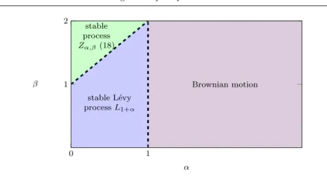
e σ2,α= Γ(1 −α) α (c − 2 +c + 2) cos π(1 +α) 2 1/(1+α) , ρe2,α= c−2 −c+2 c−2 +c+2, andc−2, c+2 given by c−2 = α 1 +α Z 0 −1| y|1+αµ(dy), c+2 = α 1 +α Z 1 0 y1+αµ(dy). (ii) If 1 +α < β <2, then asT → ∞ 1 T1−α/βℓ(T)1/βX2∗(T t) f dd → {Zα,β(t)}, where the limit{Zα,β} is a process defined as in Theorem 1(I).
Assuming that (13) and (15) hold, we can summarize the limiting behavior ofX∗
2in Figure 4. The valueα= 1 is a boundary between Gaussian and infinite variance stable limit.
Brownian motion stable L´evy processL1+α stable process Zα,β(18) 0 1 1 2 α β
Fig. 4 Classification of limits ofX∗
2
5.3 The processX3∗ SinceX∗
3 is a Gaussian process, the limiting behavior is simple (see (Grahovac, Leonenko & Taqqu 2019, Theorems 2.1 and 2.4)).
Lemma 5 (i) If Z ∞ 0 ξ−1π(dξ)<∞, then asT → ∞ 1 T1/2X3∗(T t) f dd → {eσ3B(t)}, where {B(t)} is standard Brownian motion and eσ2
3 = 2σ32 R∞
0 ξ−1π(dξ) withσ2
3= VarX3(1) =b/2.
(ii) Suppose that πhas a density psatisfying (13)with α∈(0,1) and some slowly varying function ℓ. Then asT → ∞
1
T1−α/2ℓ(T)1/2X3∗(T t)
f dd
→ {eσ3,αBH(t)},
where{BH(t)}is standard fractional Brownian motion withH = 1−α/2 andσe3,α= 2σ32(2−Γα(1+)(1α−)α) with σ
2
3 = VarX3(1) =b/2.
5.4 Proofs of Theorems 1 and 2
The limiting behavior of the integrated process X∗ follows by combining the
limit theorems of the three components in the decomposition (21). IfX∗
con-sists of at least two non-zero components, then each of these may be suitably normalized to obtain a non-trivial limiting process. However, to obtain the limit of the sum of the three components, namely the joint process X∗, one
has to take the fastest growing among the three normalizations suitable for the components. Hence, the limiting process will depend on the orders of nor-malizing sequences of the component processes. Namely, an interplay between the parametersα,β andγ will determine the limit.
Proof (Proof of Theorem 1) The proof is based on comparing the orders of normalizing sequences. LetE1andE2denote the exponents of the normalizing sequences for the processesX∗
1(T t) andX2∗(T t) respectively.
(I) If γ < 1 +α, then E1 = 1/γ by Lemma 1. It is enough to show that
T−1/γX∗
2(T t) P
→0 by showing that 1/γ > E2.
– Ifα >1, thenE2= 1/2 by Lemma 3. Sinceγ <2, 1/γ >1/2. – Ifα <1 andβ <1 +α, thenE2= 1/(1 +α) by Lemma 4(i). Since
γ <1 +α, we have 1/γ >1/(1 +α).
– If α < 1 and 1 +α < β, then E2 = 1−α/β by Lemma 4(ii). We have 1−α/β <1 + (1−γ)/β <1 + (1−γ)/γ = 1/γ.
(II) If 1 +α < γ, thenE1= 1/(1 +α) by Lemma 2. Note that implicitly we must haveα <1.
(II.a) If β < 1 +α, then E2 = 1/(1 + α) by Lemma 4(i). We have
E1 =E2 and the same normalization, hence the limit is a sum of independent limits obtained in Lemma 2 and Lemma 4(i). We additionally use (Samorodnitsky & Taqqu 1994, Property 1.2.1). (II.b) If 1 +α < β, then E2 = 1−α/β by Lemma 4(ii). We have
1−α/β >1−α/(1 +α) = 1/(1 +α)<since 1 +α < β.
Proof (Proof of Theorem 2)The proof follows the same arguments as the proof of Theorem 1.
(I) follows easily from Theorem 1 and Lemma 5. For α > 1 we conclude the statement from the fact that 1/γ > 1/2. Ifα < 1 andγ < 2/(2−α), then
γ < 1 +α, hence we need to compare 1/γ and 1−α/2. But this follows easily since 1/γ > 1−α/2 ⇔ γ < 2/(2−α). (II) follows similarly. Indeed, if 2/(2−α) < γ < 1 +α, then 1/γ < 1−α/2. If γ > 1 +α, the rate of growth of the normalizing sequence depends on β. If β < 1 +α, the order of normalizing sequence for X∗
1(T t) +X2∗(T t) is 1/(1 +α) and 1/(1 +α) = 1−α/(1 +α)<1−α/2. If 1 +α < β, the order of the normalizing sequence forX∗
1(T t) +X2∗(T t) is 1−α/β <1−α/2.
References
Bakeerathan, G. & Leonenko, N. N. (2008), ‘Linnik processes’, Random Op-erators and Stochastic Equations16(2), 109–130.
Barndorff-Nielsen, O. E. (2001), ‘Superposition of Ornstein–Uhlenbeck type processes’,Theory of Probability & Its Applications45(2), 175–194.
Barndorff-Nielsen, O. E. & Leonenko, N. N. (2005), ‘Spectral properties of su-perpositions of Ornstein-Uhlenbeck type processes’,Methodology and Com-puting in Applied Probability7(3), 335–352.
Barndorff-Nielsen, O. E., P´erez-Abreu, V. & Thorbjørnsen, S. (2013), ‘L´evy mixing’,ALEA10(2), 1013–1062.
Barndorff-Nielsen, O. E. & Stelzer, R. (2011), ‘Multivariate supOU processes’, The Annals of Applied Probability21(1), 140–182.
Barndorff-Nielsen, O. E. & Stelzer, R. (2013), ‘The multivariate supOU stochastic volatility model’,Mathematical Finance23(2), 275–296.
Barndorff-Nielsen, O. E. & Veraart, A. E. (2013), ‘Stochastic volatility of volatility and variance risk premia’, Journal of Financial Econometrics 11(1), 1–46.
Bingham, N. H., Goldie, C. M. & Teugels, J. L. (1989), Regular Variation, Vol. 27, Cambridge University Press.
Curato, I. V. & Stelzer, R. (2019), ‘Weak dependence and GMM estimation of supOU and mixed moving average processes’,Electronic Journal of Statistics 13(1), 310–360.
Eberlein, E. & Hammerstein, E. A. v. (2004), Generalized hyperbolic and inverse Gaussian distributions: limiting cases and approximation of pro-cesses, in ‘Seminar on stochastic analysis, random fields and applications IV’, Springer, pp. 221–264.
Fasen, V. & Kl¨uppelberg, C. (2007), Extremes of supOU processes,in ‘Stochas-tic Analysis and Applications: The Abel Symposium 2005’, Vol. 2, Springer Science & Business Media, pp. 339–359.
Grahovac, D., Leonenko, N. N., Sikorskii, A. & Taqqu, M. S. (2019), ‘The unusual properties of aggregated superpositions of Ornstein-Uhlenbeck type processes’,Bernoulli, in press. DOI: 10.3150/18-BEJ1044.
Grahovac, D., Leonenko, N. N. & Taqqu, M. S. (2019), ‘Limit theo-rems, scaling of moments and intermittency for integrated finite variance supOU processes’, Stochastic Processes and their Applications, in press . DOI:10.1016/j.spa.2019.01.010.
Heyde, C. & Leonenko, N. N. (2005), ‘Student processes’,Advances in Applied Probability37(2), 342–365.
Ibragimov, I. & Linnik, Y. V. (1971),Independent and Stationary Sequences of Random Variables, Wolters-Noordhoff.
Kotz, S., Kozubowski, T. J. & Podgorski, K. (2001),The Laplace Distributions and Generalizations, Birk¨auser, Boston.
Kozubowski, T. J. (2001), ‘Fractional moment estimation of Linnik and Mittag-Leffler parameters’, Mathematical and Computer Modelling 34(9-11), 1023–1035.
Kozubowski, T. J. & Panorska, A. K. (1996), ‘On moments and tail behavior of
ν-stable random variables’, Statistics & Probability Letters29(4), 307–315. Kozubowski, T. J., Podgorski, K. & Samorodnitsky, G. (1998), ‘Tails of L´evy
measure of geometric stable random variables’,Extremes1(3), 367–378. Kyprianou, A. E. (2014), Fluctuations of L´evy processes with Applications:
Moser, M. & Stelzer, R. (2013), ‘Functional regular variation of L´evy-driven multivariate mixed moving average processes’,Extremes16(3), 351–382. Pedersen, J. (2003), ‘The L´evy-Itˆo decomposition of an independently
scat-tered random measure’,MaPhySto Research Report, University of Aarhus. http://www.maphysto.dk.
Puplinskait˙e, D. & Surgailis, D. (2010), ‘Aggregation of a random-coefficient AR(1) process with infinite variance and idiosyncratic innovations’, Ad-vances in Applied Probability42(02), 509–527.
Rajput, B. S. & Rosinski, J. (1989), ‘Spectral representations of infinitely divisible processes’,Probability Theory and Related Fields82(3), 451–487. Samorodnitsky, G. & Taqqu, M. S. (1994),Stable Non-Gaussian Random
Pro-cesses: Stochastic Models with Infinite Variance, CRC press.
Sato, K. (1999), L´evy Processes and Infinitely Divisible Distributions, Cam-bridge University Press, CamCam-bridge, UK.
Stelzer, R., Tosstorff, T. & Wittlinger, M. (2015), ‘Moment based estimation of supOU processes and a related stochastic volatility model’, Statistics & Risk Modeling32(1), 1–24.
Zel’dovich, Y. B., Molchanov, S., Ruzma˘ıkin, A. & Sokolov, D. D. (1987), ‘Intermittency in random media’,Soviet Physics Uspekhi30(5), 353.