interval censoring ”case 1” via warped wavelets
Christophe Chesneau, Thomas Willer
To cite this version:
Christophe Chesneau, Thomas Willer. Estimation of a cumulative distribution function under interval censoring ”case 1” via warped wavelets. Communications in Statistics - Theory and Methods, 2015, 44 (17),<10.1080/03610926.2013.851231>. <hal-00715260v4>
HAL Id: hal-00715260
https://hal.archives-ouvertes.fr/hal-00715260v4
Submitted on 1 Dec 2013
HAL is a multi-disciplinary open access archive for the deposit and dissemination of sci-entific research documents, whether they are pub-lished or not. The documents may come from teaching and research institutions in France or abroad, or from public or private research centers.
L’archive ouverte pluridisciplinaire HAL, est destin´ee au d´epˆot et `a la diffusion de documents scientifiques de niveau recherche, publi´es ou non, ´emanant des ´etablissements d’enseignement et de recherche fran¸cais ou ´etrangers, des laboratoires publics ou priv´es.
Estimation of a cumulative distribution function
under interval censoring “case 1”
via warped wavelets
Christophe Chesneau1 and Thomas Willer2Abstract: The estimation of an unknown cumulative distribution function in the interval censoring “case 1” model from dependent sequences is considered. We construct a new adaptive estimator based on a warped wavelet basis and a hard thresholding rule. Under mild assumptions on the parameters of the model, consid-ering theL2 risk and the weighted Besov balls, we prove that the estimator attains
a sharp rate of convergence. We also investigate its practical performances thanks to simulation experiments.
Key words and phrases: Adaptive estimation, Strongly mixing, Interval censoring, Warped wavelets, Hard thresholding.
AMS 2000 Subject Classifications: 62G05, 62G20.
1
Introduction
The mathematical context of the interval censoring “case 1” model can be described as follows: let (δi, Ui)i∈Z be a strictly stationary process where, for any i∈Z,
δi=1{Xi≤Ui},
1A is the indicator function on any random event A, Xi and Ui are independent for any i, and (Xi)i∈Z is a strictly stationary process with common unknown cumulative distribution F.
We assume that U1 admits a density, denoted byg, and we denote byG its cumulative
distri-bution function. Our goal is to estimate F under mild assumptions on g from n observations (δ1, U1), . . . ,(δn, Un) of (δi, Ui)i∈Z. This model has applications in Demography and Biology.
See e.g. [14] and [19], and the references therein.
For recent statistical results, we refer to [25], [2] and [7]. In particular, considering the independent case, [2] have constructed adaptive penalized minimum contrast estimators built on trigonometric, polynomial or wavelet spaces. Using theL2 risk over Besov balls, under some
boundedness assumptions on g, [2, Corollary 3.1] proves that it attains the standard rate of convergence “n−2s/(2s+1)” wherescharacterizes the smoothness of F.
However, the independence assumption on (δi, Ui)i∈Z is often stringent in applications. In
this study, we investigate the adaptive estimation of F in a dependent setting (including the independent one). The so-called strong mixing case is considered. Examples and applications of this kind of dependence can be found in [4] and [16].
Assuming that g is known but with no boundedness assumptions on it, we develop a new adaptive estimator based on a warped wavelet basis and a hard thresholding rule. The features of this basis consist of a standard wavelet basis and of the definition ofGrelated to the model. This enables us to give a significant stability to our thresholding algorithm. Such a technique has been already used with success in the framework of nonparametric regression with random design by [20]. Recent works on warped wavelet basis in nonparametric statistics can be found in [8], [9], [3], [24], [5] and [6].
1Universit´e de Caen, LMNO, Campus II, Science 3, 14032 Caen France
Considering the L2 risk over weighted Besov balls, we prove that our estimator attains
the rate of convergence “(lnn/n)2s/(2s+1)”, where s characterizes the smoothness of F. This rate of convergence corresponds to the one attained in the i.i.d. case (see [2]) up to an extra logarithmic term. Finally, we explore the numerical performances of the estimator.
The rest of the paper is organized as follows. Section 2 introduces notations and assump-tions on the model. In Section 3, we describe warped wavelet bases on [0,1] and weighted Besov balls. Our adaptive wavelet estimator is defined in Section 4. Theoretical and practical results are presented in Section 5. The proofs are postponed to Section 6.
2
Notations and assumptions
2.1 Assumptions on the dependence structure of the process
For anym∈Z, we define them-th strongly mixing coefficient of (Xi, Ui)i∈Z by
am = sup
(A,B)∈F−∞(X,U,0)×F (X,U)
m,∞
|P(A∩B)−P(A) P(B)|, (2.1) whereF−∞(X,U,0)is theσ-algebra generated by the pairs of random variables. . . ,(X−1, U−1),(X0, U0)
and Fm,(X,U∞) is the σ-algebra generated by the random variables (Xm, Um),(Xm+1, Um+1), . . .
We consider the exponentially strongly mixing case: there exist two constants γ >0 and c >0 such that, for any integer m≥1,
am≤γexp(−cm). (2.2)
This assumption is not very restrictive; some examples of processes satisfying such conditions can be found in e.g. [26], [16], [23] and [4].
2.2 Assumptions on the densities
For the sake of simplicity, we suppose that all the considered random variables take their values in [0,1].
In the main part of the study, we assume thatg is known. The unknown case will only be explored in the simulation study in subsection 6.2.
We suppose that, for any interval [a, b]⊆[0,1], there exists a constant C >0 such that
1 b−a Z b a g(x)2dx 1/2 ≤C 1 b−a Z b a g(x)dx. (2.3)
This “reverse H¨older inequality” is related to the Muckenhoupt weights theory. It includes a wide variety of densities, non-necessarily bounded from above and/or below. For instance, g(x) = (u+ 1)xu,x ∈ [0,1] and u ∈(0,1) satisfies (2.3). Further details can be found in [20, subsection 4.1].
For any m∈ {1, . . . , n}, let f(X0,U0,Xm,Um) be the density of (X0, U0, Xm, Um),f(X0,U0) the
density of (X0, U0) and, for any (y, x, y∗, x∗)∈[0,1]4,
hm(y, x, y∗, x∗) =
f(X0,U0,Xm,Um)(y, x, y∗, x∗)−f(X0,U0)(y, x)f(X0,U0)(y∗, x∗). (2.4)
We suppose that there exists a constant C >0 such that sup m∈{1,...,n} sup (x,x∗)∈[0,1]2 1 g(x)g(x∗) Z x 0 Z x∗ 0 | hm(y, x, y∗, x∗)|dydy∗ ≤C. (2.5)
Note that, in the independent case, we havehm(y, x, y∗, x∗) = 0 and (2.5) is satisfied. Moreover,
functionsgsatisfying (2.3) and (2.5) are not necessarily bounded from below and above. Hence our conditions are less restrictive than [2, Assumption A1].
3
Warped wavelets and weighted Besov balls
Let N be a positive integer. We consider an orthonormal wavelet basis generated by dilations and translations of a ”father” Daubechies-type wavelet φ and a ”mother” Daubechies-type wavelet ψ of the family db2N (see [11]). In particular, mention that φ and ψ have compact supports.
We set
φj,k(x) = 2j/2φ(2jx−k), ψj,k(x) = 2j/2ψ(2jx−k). Suppose that (2.3) holds and recall that
G(x) =P(U1 ≤x) =
Z x
0
g(u)du, x∈R.
Then, with an appropriate treatment at the boundaries, there exists an integerτ satisfying 2τ ≥ 2N such that, for any integer j∗ ≥ τ, any h ∈L2([0,1]) =
n
h: [0,1]→R; R1
0 h2(x)dx <∞ o
can be expanded into a warped wavelet series as
h(x) = 2j∗−1 X k=0 αj∗,kφj∗,k(G(x)) + ∞ X j=j∗ 2j−1 X k=0 βj,kψj,k(G(x)), x∈[0,1], where αj,k = Z 1 0 h(G−1(x))φj,k(x)dx, βj,k = Z 1 0 h(G−1(x))ψj,k(x)dx. (3.1) See [20, subsection 3.3].
LetM >0 and s >0. We say that a functionhinL2([0,1]) belongs to the weighted Besov
ball Bs,w∞(M) if there exists a constant M > 0 such that the associated wavelet coefficients (3.1) satisfy, for any integerj ≥τ,
2j−1 X k=0 βj,k2 wj,k ≤M2−j(2s+1), where wj,k = Z (k+1)/2j k/2j 1 g(G−1(x))dx. (3.2)
In this expression, s is a smoothness parameter. Details concerning the warped wavelets and the analytic definition of weighted Besov balls can be found in [20, Section 7]. For the standard wavelet basis on [0,1], see e.g. [22] and [10].
4
Estimators
For any integer j ≥τ and any k ∈ {0, . . . ,2j −1}, we estimate the unknown warped wavelet coefficients of F i.e. αj,k = R01F(G−1(x))φj,k(x)dx and βj,k = R01F(G−1(x))ψj,k(x)dx by respectively ˆ αj,k = 1 n n X i=1 δiφj,k(G(Ui)), βˆj,k = 1 n n X i=1 δiψj,k(G(Ui)). (4.1)
We estimate F by the following hard thresholding estimator ˆF: ˆ F(x) = 2j0−1 X k=0 ˆ αj0,kφj0,k(G(x)) + j1 X j=j0 2j−1 X k=0 ˆ βj,k1{|βˆj,k|≥κρn}ψj,k(G(x)), (4.2) wherex∈[0,1], j0 is an integer such that
1
2lnn <2
j0 ≤lnn,
ˆ
αj0,k and ˆβj,k are defined by (4.1), j1 is the integer satisfying
1 2 n (lnn)3 <2 j1 ≤ n (lnn)3, (4.3)
κ is a large enough constant (the one in Proposition 6.3 below) and ρn denotes the “universal threshold”, i.e.
ρn=
r
lnn
n . (4.4)
Naturally, for x <0, we put ˆF(x) = 0 and, forx >1, ˆF(x) = 1.
Note that ˆF is adaptive: its construction does not depend on the smoothness ofF. The general idea in the construction of ˆF is to apply a term-by-term selection on the unknown wavelet coefficients of F: only the most significant are kept. The reason is that only these few coefficients contain the main characteristics ofF. For the construction of hard thresholding wavelet estimators in the standard nonparametric models, see e.g. [15], [13] and [18].
When g is unknown, an intuitive adaptive estimator of F is (4.2) but, instead of G, we consider its empirical version:
ˆ Gn(x) = 1 n n X i=1 1{Ui≤x}.
This plug-in method yields the hard thresholding estimator ˆ F∗(x) = 2j0−1 X k=0 ˆ α∗j0,kφj0,k( ˆGn(x)) + j1 X j=j0 2j−1 X k=0 ˆ βj,k∗ 1{|βˆj,k|≥κρn}ψj,k( ˆGn(x)), (4.5) x∈[0,1], where ˆ α∗j,k = 1 n n X i=1 δiφj,k( ˆGn(Ui)), βˆ∗j,k = 1 n n X i=1 δiψj,k( ˆGn(Ui)).
We do not investigate the theoretical performances of this estimator, but we use it throughout the simulation and real data study of Section 5.2.
5
Performances of
F
ˆ
5.1 Theoretical results
Theorem 5.1 Suppose that the assumptions of Section 2 hold. Let Fˆ be (4.2). Suppose that F ∈Bw
s,∞(M) with s >0. Then there exists a constant C >0 such that
E Z 1 0 ˆ F(x)−F(x)2dx ≤C lnn n 2s/(2s+1) .
The proof of Theorem 5.1 uses a suitable decomposition of the L2 risk including some
geo-metrical properties of the warped wavelet basis and the statistical properties of the wavelet coefficients estimators presented in Propositions 6.1, 6.2 and 6.3.
Theorem 5.1 shows that, under mild assumptions on the dependence of the observations and on g, ˆF attains a rate of convergence close to the one for the i.i.d. case i.e. n−2s/(2s+1). The difference is the “negligible” logarithmic term (lnn)2s/(2s+1).
Let us recall that, if we restrict our study to the independent case, contrary to [2, Assump-tion A1], Theorem 5.1 holds without boundedness assumpAssump-tions on g.
5.2 Practical results
This section is devoted to the numerical performances of ˆF. We restrict ourselves to the i.i.d. case: no exponentially strongly mixing hypothesis is made here.
5.2.1 Preliminary remarks on the estimators
In practice, the construction and the performances of the two estimators in the case of known or unknown design density are very close. Thus for the sake of brevity, we present only the results for the unknown design density procedure.
We compare the performances of the warped wavelet estimator to those of the piecewise polynomial regression estimator developped in [2]. Another procedure, named quotient esti-mator, is also proposed in that paper. However it is generally outperformed by the regression estimator, so we focus only on the warped wavelet and the piecewise polynomial estimators. We name them respectively WWE and PPE in the sequel. We give examples of their behaviours when applied to various simulated data sets and to one real data set.
In both methods, one needs to fit several preliminary parameters. For the WWE, the calibration of the threshold κρn and of the cutoff level j1 are important practical issues. The
values given by the theory are not useful in practice. Indeed the thresholds are defined up to some intricate ”large enough constant κ”. Moreover the cutoff level j1 defined in (4.3) is too
small in practice, as it is even lower than the minimal coarsest level value. Thus, forj1, we use
j1 = log2(n)−1, i.e. the maximal possible level, hoping the high resolution ”noise” is filtered
thanks to thresholding.
For the thresholds, we can use an analogy with the non-parametric regression model in random design. Indeed the censoring model amounts to observing at each design point Ui some Bernoulli variableδi with (conditionally toUi) expectationF(Ui) and standard deviation
p
F(Ui)(1−F(Ui)). In the usual regression model one observes at each design pointUi some Gaussian variable δi with (conditionally to Ui) expectation F(Ui) and some given standard errorσ. Thus we calibrate κ as in regression (see [9]) as the following random value:
κr= v u u t 1 n−2 n X i=2 (δ(i)−δ(i−1))2,
where each δ(i) refers to the value δk such that Uk is the i-th higher coordinate of the vector (Uj)1≤j≤n. Nevertheless, the standard error is highly heteroscedastic in the censoring problem: it varies from 0 for observations near the edges of the observation interval, to 0.5 near the median of F. Thus we also use a more conservative deterministic threshold corresponding to
κd= 0.5× √
2 = √1 2.
Thus, we make sure that the high noise of the median observations is well taken into account in the thresholds. In the sequel, we name the random threshold estimator WWEr and the deterministic threshold estimator WWEd.
Lastly, we use the ’Daubechies 4’ wavelet basis for the simulated data study, and the ’Daubechies 3’ wavelet basis for the real data study (as the number of observations is a bit small for Daubechies 4 basis).
The PPE also requires to fix some preliminary parameters. First some maximal degree of the polynomials and some maximal numbers of intervals must be put as arguments. We choose the degree as equal to 6 and maximum number of intervals as equal to 64 for the simulated data, and to 32 for the real data. Secondly some noise variance level must be put as an argument as well. We make two choices corresponding to the random and deterministic values used for WWEr and WWEd. Likewise, in the sequel, we name the corresponding estimators PPEr and PPEd.
Hence for each data set we compare the performances of four estimators: WWEr, WWEd, PPEr and PPEd.
Concerning the programs, the WWE is very simple to implement in practice. The program consists mainly in simple wavelet decompositions or recompositions, computations of thresholds, and shrinkage of some small wavelets coefficients. The PPE was implemented thanks to the FY3P.m Matlab file and several other sub-programs (all available on Yves Rozenholc’s web page). The implementation is much more complex, as can be seen from the programs. What is more, the processing times necessary to compute the estimators are very different. For example one needs a CPU time of 0.078 to compute the eight Warped Wavelets Estimators represented in Figure 5.2.2, whereas one needs a CPU time of 670.49 to compute the eight Piecewise Polynomial Estimators built on the same data and represented in the same figure.
5.2.2 Study with simulated data
Simulation of the data
We consider four target functionsF which correspond to the following formula with values q= 0.2,1,5,50:
Fq(t) =
(
2q−1tq, t∈[0,0.5],
1−2q−1(1−t)q, t∈[0.5,1]. (5.1) These four functions are plotted in Figure 1. Furthermore we consider five different densities of the Uis. We name them Bump1, Bump2, Pit1, Pit2 and Uniform. They correspond to the following formulas (up to normalization constants), and are plotted in Figure 2.
• Bump1g(x) = exp(−(100∗(x−0.5)2)) + 1,
• Pit1 g(x) =−exp(−(100∗(x−0.5)2)) + 1.05,
• Bump2g(x) = exp(−(100∗x2)) + exp(−(100∗(x−1)2)) + 1,
• Pit2 g(x) =−exp(−(100∗x2))−exp(−(100∗(x−1)2)) + 1.05, • Uniformg(x) = 1.
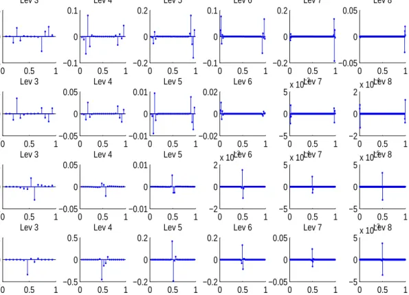
The non uniform densities correspond to a surplus or a lack of design points near the edges or near the middle of the interval. The WWE should normally capture detail coefficients in zones of dense design, and fail to do so in low design density zones. Nevertheless, this design effect can be counterbalanced by the variations of the level of noise in the observation, as mentioned previously. Thus it is difficult to predict the performances of the estimator, especially in the middle of the interval. As an example, the wavelet detail coefficients of the targets are plotted in Figure 3. One can remark that Fq has high detail coefficients near the edges of the interval [0,1] when q is small, and at the middle of the interval [0,1] when q is large. One can expect estimation problems for example for the F5 or F50 functions in the case of the ’Pit1’ design
0 0.5 1 0 0.5 1 0 0.5 1 0 0.5 1 0 0.5 1 0 0.5 1 0 0.5 1 0 0.5 1
Figure 1: Four target cumulative distribution functions: F0.2,F1,F5,F50 (from left to right)
0 0.5 1 0 0.5 1 1.5 2 Bump1 0 0.5 1 0 0.5 1 1.5 2 Pit1 0 0.5 1 0 0.5 1 1.5 2 Bump2 0 0.5 1 0 0.5 1 1.5 2 Pit2 0 0.5 1 0 0.5 1 1.5 2 Uniform
Figure 2: Densities of the (Ui)s: Bump1, Pit1, Bump2, Pit2 and Uniform (from left to right)
0 0.5 1 −0.5 0 0.5 Lev 3 0 0.5 1 −0.1 0 0.1 Lev 3 0 0.5 1 −0.2 0 0.2 Lev 3 0 0.5 1 −2 0 2 Lev 3 0 0.5 1 −0.1 0 0.1 Lev 4 0 0.5 1 −0.05 0 0.05 Lev 4 0 0.5 1 −0.05 0 0.05 Lev 4 0 0.5 1 −0.5 0 0.5 Lev 4 0 0.5 1 −0.2 0 0.2 Lev 5 0 0.5 1 −0.01 0 0.01 Lev 5 0 0.5 1 −0.01 0 0.01 Lev 5 0 0.5 1 −0.2 0 0.2 Lev 5 0 0.5 1 −0.1 0 0.1 Lev 6 0 0.5 1 −0.02 0 0.02 Lev 6 0 0.5 1 −2 0 2x 10 −3 Lev 6 0 0.5 1 −0.2 0 0.2 Lev 6 0 0.5 1 −0.2 0 0.2 Lev 7 0 0.5 1 −5 0 5x 10 −3 Lev 7 0 0.5 1 −5 0 5x 10 −4 Lev 7 0 0.5 1 −0.05 0 0.05 Lev 7 0 0.5 1 −0.05 0 0.05 Lev 8 0 0.5 1 −2 0 2x 10 −4 Lev 8 0 0.5 1 −5 0 5x 10 −5 Lev 8 0 0.5 1 −5 0 5x 10 −3 Lev 8
Figure 3: Detail wavelet coefficients of each target function: the first row relates toF0.2, the second toF1, the
0 0.1 0.2 0.3 0.4 0.5 0.6 0.7 0.8 0.9 1 0 0.2 0.4 0.6 0.8 1
Figure 4: Data with (Ui)s (uniformly distributed) on axis 1, and their corresponding (δi)s on axis 2, for the F50function. 0 0.5 1 −2 −1 0 1 2 Lev 3 0 0.5 1 −2 −1 0 1 2 Lev 3 0 0.5 1 −2 −1 0 1 2 Lev 4 0 0.5 1 −2 −1 0 1 2 Lev 4 0 0.5 1 −2 −1 0 1 2 Lev 5 0 0.5 1 −2 −1 0 1 2 Lev 5 0 0.5 1 −2 −1 0 1 2 Lev 6 0 0.5 1 −2 −1 0 1 2 Lev 6 0 0.5 1 −2 −1 0 1 2 Lev 7 0 0.5 1 −2 −1 0 1 2 Lev 7 0 0.5 1 −2 −1 0 1 2 Lev 8 0 0.5 1 −2 −1 0 1 2 Lev 8
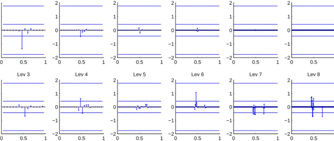
Figure 5: Random thresholds (lower horizontal bars), deterministic thresholds (higher horizontal bars), wavelet detail coefficients ofF50(first row of graphics), wavelet detail coefficients of the (δi)s (second row of graphics)
An example of data and wavelet estimator
An example of the data on which the estimators are based is given in Figures 4 and 5 (for the cdfF50 and for a uniform distribution of theUis). Figure 4 represents the couples (Ui, δi). The second row of Figure 5 gives the detail wavelet coefficients of the sequence (δσU(i))i∈{1,...,n},
whereσU is the following permutation: σU(i) is the indexjsuch thatUj is theistlargest element of the sequenceU. These coefficients are approximations of the ones given in equation (4.1), as their construction consists in replacing G by the empirical pdf ˆGn in their expressions. They should be estimations of the coefficients of the target function, which are plotted in the first row of Figure 5. Then the estimation consists in trying to select the coefficients corresponding to the signal F, and to put to zero those corresponding to the ”noise”.
As one can see from Figure 5, the thresholding is a hard task as the coefficients of the data are significantly different from the target coefficients. This may stem from the high noise of the observations in the middle of the interval, as discussed previously. The deterministic threshold is conservative as all the detail coefficients are thresholded. The random threshold is too low and leaves high resolution noise unfiltered. The corresponding estimators can be seen in Figure 6, and WWEr indeed contains artefacts in the middle of the interval.
Some examples of results
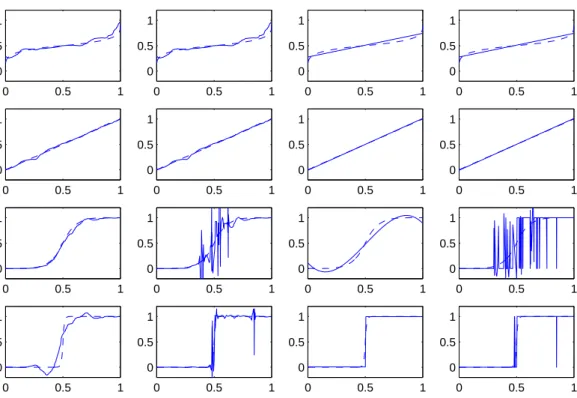
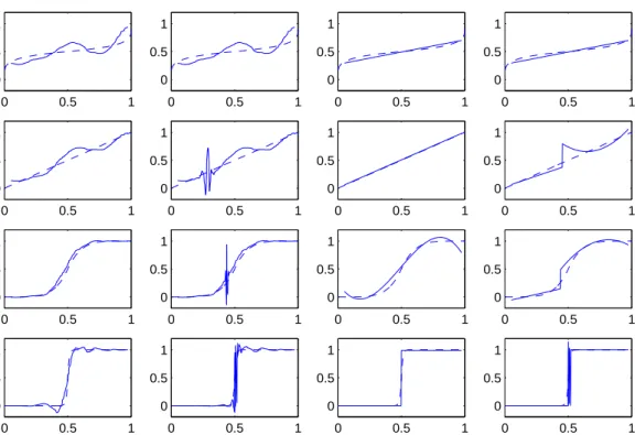
We give examples of realizations of the 4 estimators for all the 20 simulated data sets. Figures 6, 7, 8, 9, 10 give examples for respectively the Uniform, Bump1, Pit1, Bump2, and Pit2 design densities. Each figure represents the target function (dashed line) and the estimator (solid line). We can draw the following conclusions.
• All the estimators behave rather properly at the edges of the interval, while there are sometimes problems in the middle of the interval. This is coherent with the variations of the noise variance, as discussed previously. As one could expect, the random threshold estimators have poor performances in the middle of the interval for the Uniform and Pit1 designs.
• Generally, the deterministic threshold estimators are better than the random threshold estimators. Probably the latter underestimate the noise level in the middle of the interval, and thus their performances are poor, especially when the number of observations in this zone is small.
• For the F0.2 or F1 targets, all the estimators are generally rather close. One can remark
however that PPE is a bit better than WWE. One can check that they consist of rough approximation methods: for WWE all the detail coefficients are cut, and for PPE low degree polynomials and few intervals are selected. For WWE, one may ask oneself if the results could be improved by using other calibrations ofκ and j1. For this purpose, one
can compute some ”oracle” estimator in the sense that it uses the threshold and the cutoff values which minimize the mean square error among all estimators of the type of Section 4, except with κ and j1 left free. Of course this estimator is completely inaccessible in
practice. Monte Carlo approximations of the mean square error show that the oracle strategy consists in putting all the detail coefficients to zero. Thus these two functions probably lead to globally noisy observations, and it must be hopeless to try to recover details of the targets in these cases.
• For theF5 target, WWE generally outperforms PPE. However, for theF50 target, PPE
generally outperforms WWE.
5.2.3 Study with real data
We use a data set concerning a tumorigenicity experiment conducted by the National Toxicology Program (NTP) which is described and summarized in Dunson and Dinse (2002). There are four sets of data. We use only the one corresponding to the ’control’ group and the presence of adrenal tumor. The subjects were fifty rats or mice. TheXis are unobserved dates of occurrence of an adrenal tumor and the Ui are dates of death. Every month during 25 months, all the dead mice or rats were examined to check if they had a tumor or not, which corresponds to respectivelyδi = 1 and δi = 0. The experience stopped after the 25th month (we consider this date as the 26th month) when all the remaining were killed and examined.
Several remarks need to be made on this data set. First at month 26 the data show that 5 out of the 13 remaining mice had no tumor, thus the upper bound of the support ofF was not reached. This is why in the sequel, our estimators stop at about 0.7 and not 1. Secondly, the design dates cannot be considered as realizations of continuous random variables. In particular, since the observations are gathered by months, several deaths occurred at exactly the same time. Thus we considered that all the deaths at month m were in fact distributed on a regular grid between monthsm−1 and m.
The four estimators are plotted in Figure 11. The two thresholding techniques yield to the same estimator. The PPE yields a rough one degree polynomial estimation, whereas the WWE yields a more detailed curve.
0 0.5 1 0 0.5 1 0 0.5 1 0 0.5 1 0 0.5 1 0 0.5 1 0 0.5 1 0 0.5 1 0 0.5 1 0 0.5 1 0 0.5 1 0 0.5 1 0 0.5 1 0 0.5 1 0 0.5 1 0 0.5 1 0 0.5 1 0 0.5 1 0 0.5 1 0 0.5 1 0 0.5 1 0 0.5 1 0 0.5 1 0 0.5 1 0 0.5 1 0 0.5 1 0 0.5 1 0 0.5 1 0 0.5 1 0 0.5 1 0 0.5 1 0 0.5 1
Figure 6: Uniform design: estimators WWEd, WWEr, PPEd, PPEr (left to right) for targetsF0.2,F1,F5,F50
(from top to bottom)
0 0.5 1 0 0.5 1 0 0.5 1 0 0.5 1 0 0.5 1 0 0.5 1 0 0.5 1 0 0.5 1 0 0.5 1 0 0.5 1 0 0.5 1 0 0.5 1 0 0.5 1 0 0.5 1 0 0.5 1 0 0.5 1 0 0.5 1 0 0.5 1 0 0.5 1 0 0.5 1 0 0.5 1 0 0.5 1 0 0.5 1 0 0.5 1 0 0.5 1 0 0.5 1 0 0.5 1 0 0.5 1 0 0.5 1 0 0.5 1 0 0.5 1 0 0.5 1
Figure 7: Bump1 design: estimators WWEd, WWEr, PPEd, PPEr (left to right) for targetsF0.2,F1,F5,F50
0 0.5 1 0 0.5 1 0 0.5 1 0 0.5 1 0 0.5 1 0 0.5 1 0 0.5 1 0 0.5 1 0 0.5 1 0 0.5 1 0 0.5 1 0 0.5 1 0 0.5 1 0 0.5 1 0 0.5 1 0 0.5 1 0 0.5 1 0 0.5 1 0 0.5 1 0 0.5 1 0 0.5 1 0 0.5 1 0 0.5 1 0 0.5 1 0 0.5 1 0 0.5 1 0 0.5 1 0 0.5 1 0 0.5 1 0 0.5 1 0 0.5 1 0 0.5 1
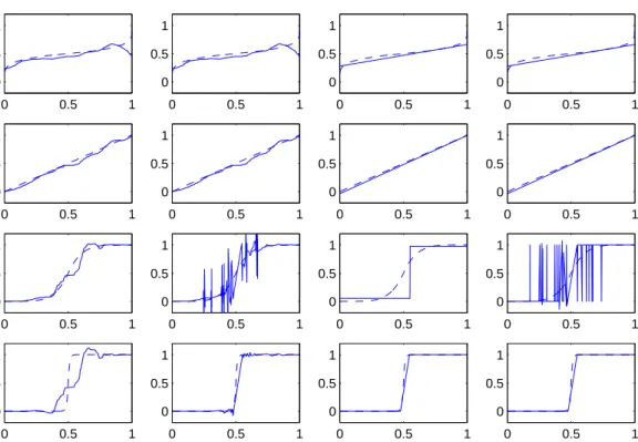
Figure 8: Pit1 design: estimators WWEd, WWEr, PPEd, PPEr (left to right) for targetsF0.2,F1, F5,F50
(from top to bottom)
0 0.5 1 0 0.5 1 0 0.5 1 0 0.5 1 0 0.5 1 0 0.5 1 0 0.5 1 0 0.5 1 0 0.5 1 0 0.5 1 0 0.5 1 0 0.5 1 0 0.5 1 0 0.5 1 0 0.5 1 0 0.5 1 0 0.5 1 0 0.5 1 0 0.5 1 0 0.5 1 0 0.5 1 0 0.5 1 0 0.5 1 0 0.5 1 0 0.5 1 0 0.5 1 0 0.5 1 0 0.5 1 0 0.5 1 0 0.5 1 0 0.5 1 0 0.5 1
Figure 9: Bump2 design: estimators WWEd, WWEr, PPEd, PPEr (left to right) for targetsF0.2,F1,F5,F50
0 0.5 1 0 0.5 1 0 0.5 1 0 0.5 1 0 0.5 1 0 0.5 1 0 0.5 1 0 0.5 1 0 0.5 1 0 0.5 1 0 0.5 1 0 0.5 1 0 0.5 1 0 0.5 1 0 0.5 1 0 0.5 1 0 0.5 1 0 0.5 1 0 0.5 1 0 0.5 1 0 0.5 1 0 0.5 1 0 0.5 1 0 0.5 1 0 0.5 1 0 0.5 1 0 0.5 1 0 0.5 1 0 0.5 1 0 0.5 1 0 0.5 1 0 0.5 1
Figure 10: Pit2 design: estimators WWEd, WWEr, PPEd, PPEr (left to right) for targetsF0.2,F1,F5,F50
(from top to bottom)
10 15 20 25 30 35 0 0.5 1 10 15 20 25 30 35 0 0.5 1 10 15 20 25 30 35 0 0.5 1 10 15 20 25 30 35 0 0.5 1
5.3 Conclusion and discussion
In this paper we develop a new adaptive estimator for the cumulative distribution function under interval censoring “case 1” for possible dependent data. It is constructed from warped wavelet basis and a hard thresholding rule. Theoretical results show the good performance of our estimator under mild assumptions on the model (including vanishing density g). The practical performances were investigated thanks to a comparison with the estimator developped in [2]. The wavelet estimator displays generally satisfying performances, provided a conservative calibration of the threshold is made. Moreover it is simpler and faster to compute than the estimator of [2].
Possible perspectives of this work are to
• determine the rate of convergence of ˆF∗ (4.5) under the L2 risk over Besov balls,
• relax assumptions (2.2) and/or (2.5),
• improve the obtained rate of convergence by considering more sophisticated thresholding rules as those developed in [1].
6
Proofs
In this section, we suppose that the assumptions of Section 2 hold. Moreover, C denotes any constant that does not depend on j,k and n. Its value may change from one term to another and may depend on φor ψ.
6.1 Auxiliary results on (4.1)
Proposition 6.1 Suppose that the assumptions of Section2 hold. For any integer j≥j0 such
that 2j ≤n and any k∈ {0, . . . ,2j −1}, let αj,k =
R1
0 F(G−1(x))φj,k(x)dx and αˆj,k be defined
as in (4.1). Then αˆj,k is an unbiased estimator for αj,k and there exists a constant C >0 such that
Var(ˆαj,k)≤C 1 n,
Let us mention that Proposition 6.1 can be proved with ˆβj,k (4.1) instead of αj,k and βj,k =R01F(G−1(x))ψj,k(x)dxinstead ofαj,k.
Proof of Proposition 6.1. We have
E(ˆαj,k) = E(δ1φj,k(G(U1))) = E 1{Xi≤Ui}φj,k(G(U1))
= Z 1 0 Z u 0 f(x)φj,k(G(u))g(u)dxdu= Z 1 0 F(u)φj,k(G(u))g(u)du = Z 1 0 F(G−1(u))φj,k(u)du=αj,k.
An elementary covariance inequality yields Var (ˆαj,k) = 1 n2 n X v=1 n X ℓ=1
Cov (δvφj,k(G(Uv)), δℓφj,k(G(Uℓ)))≤S+T, (6.1) where
S= 1
and T= 2 n2 n X v=2 v−1 X ℓ=1
Cov (δvφj,k(G(Uv)), δℓφj,k(G(Uℓ)))
. Since δ1 ≤1, we have S ≤ 1 nE (δ1φj,k(G(U1)))2 ≤ 1 nE (φj,k(G(U1))) 2 = 1 n Z 1 0 (φj,k(G(x)))2g(x)dx= 1 n Z 1 0 (φj,k(x))2dx= 1 n. (6.2)
It follows from the stationarity of (δi, Ui)i∈Z and 2j ≤nthat
T = 2 n2 n X m=1
(n−m) Cov (δ0φj,k(G(U0)), δmφj,k(G(Um)))
≤ 2 n n X m=1
|Cov (δ0φj,k(G(U0)), δmφj,k(G(Um)))|=T1+T2, (6.3)
where T1 = 2 n 2j−1 X m=1
|Cov (δ0φj,k(G(U0)), δmφj,k(G(Um)))| and T2= 2 n n X m=2j
|Cov (δ0φj,k(G(U0)), δmφj,k(G(Um)))|.
Upper bound for T1. Using (2.4), (2.5) and the change of variablesy= 2jx−k, we obtain
|Cov (δ0φj,k(G(U0)), δmφj,k(G(Um)))| = Z 1 0 Z 1 0 Z 1 0 Z 1 0 hm(y, x, y∗, x∗) 1{y≤x}φj,k(G(x))1{y∗≤x∗}φj,k(G(x∗)) dydxdy∗dx∗ ≤ Z 1 0 Z x∗ 0 Z 1 0 Z x 0 | hm(y, x, y∗, x∗)| |φj,k(G(x))φj,k(G(x∗))|dydxdy∗dx∗ ≤ C Z 1 0 | φj,k(G(x))|g(x)dx 2 ≤C Z 1 0 | φj,k(x)|dx 2 ≤C2−j. Therefore T1≤C 1 n2 −j2j =C1 n. (6.4)
Upper bound for T2. Applying the Davydov inequality for strongly mixing processes (see [12]),
for any q∈(0,1), we have
|Cov (δ0φj,k(G(U0)), δmφj,k(G(Um)))| ≤ CaqmE|δ0φj,k(G(U0))|2/(1−q) 1−q ≤CaqmE|φj,k(G(U0))|2/(1−q) 1−q ≤ Caqm sup x∈[0,1]| φj,k(G(x))| !2q E(φj,k(G(U0)))2 1−q .
We have supx∈[0,1]|φj,k(x)| ≤C2j/2 and, by (6.2), E(φj,k(G(U0)))2
Therefore
|Cov (δ0φj,k(G(U0)), δmφj,k(G(Um)))| ≤C2qjaqm. Hence T2≤C 1 n2 qj n X m=2j aqm ≤C1 n n X m=2j mqaqm≤C1 n. (6.5)
It follows from (6.3), (6.4) and (6.5) that
T≤C1
n. (6.6)
Combining (6.1), (6.2) and (6.6), we obtain
Var ( ˆαj,k)≤C 1 n. The proof of Proposition 6.1 is complete.
Proposition 6.2 Suppose that the assumptions of Section2 hold. For any integer j≥j0 such
that 2j ≤n and any k∈ {0, . . . ,2j−1}, let βj,k =
R1
0 F(G−1(x))ψj,k(x)dx and βˆj,k be defined
as in (4.1). Then there exists a constant C >0 such that
E ˆ βj,k−βj,k 4 ≤C2j1 n.
Proof of Proposition 6.2. Observe that
|βˆj,k−βj,k| ≤ |βˆj,k|+|βj,k| ≤ sup (x,y)∈[0,1]2| yψj,k(G(x))|+C ≤ sup x∈[0,1]| ψj,k(x)|+C ≤C2j/2. (6.7)
Using (6.7) and Proposition 6.1, we obtain E ˆ βj,k−βj,k 4 ≤C2jE ˆ βj,k−βj,k 2 ≤C2j1 n. The proof of Proposition 6.2 is complete.
Proposition 6.3 Suppose that the assumptions of Section2hold. For any j∈ {j0, . . . , j1}and
any k∈ {0, . . . ,2j−1}, letβ
j,k =R01F(G−1(x))ψj,k(x)dx, βˆj,k be (4.1) and ρn be defined as in (4.4). Then there exist two constants, κ >0 and C >0, such that
P|βˆj,k−βj,k| ≥κρn/2
≤C 1 n4.
Proof of Proposition 6.3. We shall use the Bernstein inequality for exponentially strongly mixing process presented in Lemma 6.1 below. The proof can be found in [21].
Lemma 6.1 ([21]) Let γ >0, c >0 and (Zi)i∈Z be a strictly stationary process defined on a
probability space (Ω,A,P) with the m-th strongly mixing coefficient (2.1). Let n be a positive integer, h:R→ R be a measurable function and, for any i∈Z, Vi =h(Zi). We assume that
E(V1) = 0and there exists a constantM >0satisfying|V1| ≤M. Then, for anym∈ {1, . . . , n}
and any λ >0, we have
P 1 n n X i=1 Vi ≥λ ! ≤4 exp − λ 2n 16(Dm/m+λM m/3) + 32M λ nam,
where Dm= maxl∈{1,...,2m}Var
Pl
i=1Vi
. For anyi∈ {1, . . . , n}, set
Vi=δiψj,k(G(Ui))−βj,k. Then P|βˆj,k−βj,k| ≥κρn/2 = P 1 n n X i=1 Vi ≥κρn/2 ! , (6.8)
V1, . . . , Vn are identically distributed, depend on the strictly stationary strongly mixing process (δi, Ui)i∈Z satisfying (2.2), Propositions 6.1 and 6.2 give
E (V1) = 0, E V12
≤E(δ1φj,k(G(U1)))2
≤1,
and, using similar arguments to (6.7), |V1| ≤ C2j/2 ≤ C2j1/2 ≤ C(n/(lnn)3)1/2. Now set
m= [ulnn] with u > 0 (chosen later). Proceeding as in the bounds ofS and T1 in the proof
of Proposition 6.1 withl instead of n, we have
max l∈{1,...,2m}Var l X i=1 Vi ! ≤ C max l∈{1,...,2m}(l+l 22−j)≤C max l∈{1,...,2m}(l+l 22−j0) ≤ C m+ m 2 lnn ≤Cm.
It follows from Lemma 6.1 applied with these V1, . . . , Vn, λ = κCρn, ρn = (lnn/n)1/2, m=ulnnwithu >0 (chosen later), M =C(n/(lnn)3)1/2 and (2.2) that
P|βˆj,k−βj,k| ≥κρn/2 ≤ C exp −C κ 2ρ2 nn 1 +κρnmM + n 1/2 ρn(lnn)3/2 nexp(−cm) ! ≤ C exp −C κ 2lnn 1 +κ(lnn/n)1/2ulnn(n/(lnn)3)1/2 +n2exp(−culnn) ≤ Cn−Cκ2/(1+κu)+n2−cu.
Taking κand u large enough, we obtain
P|βˆj,k−βj,k| ≥κρn/2
≤C 1 n4.
This ends the proof of Proposition 6.3.
6.2 Proof of Theorem 5.1
Proof of Theorem 5.1. Since F ∈L2([0,1]), we can write
F(x) = 2j0−1 X k=0 αj0,kφj0,k(G(x)) + ∞ X j=j0 2j−1 X k=0 βj,kψj,k(G(x)), x∈[0,1], whereαj0,k = R1 0 F(G−1(x))φj0,k(x)dxand βj,k = R1 0 F(G−1(x))ψj,k(x)dx.
We have, for any x∈[0,1], ˆ F(x)−F(x) = 2j0−1 X k=0 (ˆαj0,k−αj0,k)φj0,k(G(x)) + j1 X j=j0 2j−1 X k=0 ˆ βj,k1{|βˆj,k|≥κρn} −βj,k ψj,k(G(x)) − ∞ X j=j1+1 2j−1 X k=0 βj,kψj,k(G(x)).
We now need the following lemma which is an immediate consequence of [20, Lemma 2] and the Minkowski inequality.
Lemma 6.2 ([20]) Suppose that (2.3) holds. Then, for any sequences (uj,k)∈ℓ2(N2)and any
integers j0 and j1 such that j1 > j0 ≥j0, there exists a constant C >0 such that
Z 1 0 j1 X j=j0 2j−1 X k=0 uj,kψj,k(G(x)) 2 dx≤C j1 X j=j0 2j/2 2j−1 X k=0 u2j,kwj,k 1/2 2 , where wj,k is defined by (3.2).
It follows from Lemma 6.2 and the Cauchy-Schwarz inequality that E Z 1 0 ˆ F(x)−F(x)2dx ≤C(F+G+H), (6.9) where F= 2j0 2j0−1 X k=0 E(ˆαj0,k−αj0,k) 2 wj0,k, G= j1 X j=j0 2j/2 2j−1 X k=0 E ˆ βj,k1{|βˆj,k|≥κρn} −βj,k 2 wj,k 1/2 2 and H= ∞ X j=j1+1 2j/2 2j−1 X k=0 βj,k2 wj,k 1/2 2 .
Using Proposition 6.1 and P2j0−1
k=0 wj0,k= 1, we obtain F≤C1 n2 j0 2j0−1 X k=0 wj0,k ≤C lnn n ≤C lnn n 2s/(2s+1) . (6.10)
Since F ∈Bs,w∞(M), we have H ≤ C ∞ X j=j1+1 2−js 2 ≤C2−2j1s≤C (lnn)3 n 2s ≤ C lnn n 2s/(2s+1) . (6.11)
Let us now bound the termG. Observe that
G≤C(G1+G2+G3+G4), (6.12) where G1 = j1 X j=j0 2j/2 2j−1 X k=0 E ˆ βj,k−βj,k 2 1{|βˆj,k|≥κρn}1{|βj,k|<κρn/2} wj,k 1/2 2 , G2 = j1 X j=j0 2j/2 2j−1 X k=0 E ˆ βj,k−βj,k 2 1{|βˆj,k|≥κρn}1{|βj,k|≥κρn/2} wj,k 1/2 2 , G3 = j1 X j=j0 2j/2 2j−1 X k=0 Eβj,k2 1{|βˆj,k|<κρn}1{|βj,k|≥2κρn} wj,k 1/2 2 and G4 = j1 X j=j0 2j/2 2j−1 X k=0 Eβj,k2 1{|βˆj,k|<κρn}1{|βj,k|<2κρn} wj,k 1/2 2 .
Upper bounds for G1+G3. Note that n |βˆj,k|< κρn, |βj,k| ≥2κρn o ⊆n|βˆj,k−βj,k|> κρn/2 o , n |βˆj,k| ≥κρn, |βj,k|< κρn/2 o ⊆n|βˆj,k−βj,k|> κρn/2 o and n |βˆj,k|< κρn, |βj,k| ≥2κρn o ⊆n|βj,k| ≤2|βˆj,k−βj,k| o . So G1+G3 ≤C j1 X j=j0 2j/2 2j−1 X k=0 E ˆ βj,k−βj,k 2 1{|βˆj,k−βj,k|>κρn/2} wj,k 1/2 2 .
It follows from the Cauchy-Schwarz inequality, Proposition 6.2, Proposition 6.3 and 2j ≤2j1 ≤n
that E ˆ βj,k−βj,k 2 1{|βˆj,k−βj,k|>κρn/2} ≤ E ˆ βj,k−βj,k 41/2 P|βˆj,k−βj,k|> κρn/2 1/2 ≤ C 2j1 n 1/2 1 n4 1/2 ≤C 1 n2.
Since P2j−1 k=0 wj,k = 1, we have G1+G3 ≤ C 1 n2 j1 X j=j0 2j/2 2j−1 X k=0 wj,k 1/2 2 =C 1 n2 j1 X j=j0 2j/2 2 ≤ C 1 n22 j1 ≤C1 n ≤C lnn n 2s/(2s+1) . (6.13)
Upper bound for G2. Using again Proposition 6.2, we obtain
E ˆ βj,k−βj,k 2 ≤C1 n ≤C lnn n . Hence G2≤C lnn n j1 X j=j0 2j/2 2j−1 X k=0 1{|β j,k|>κρn/2}wj,k 1/2 2 .
Letj2 be the integer defined by
1 2 n lnn 1/(2s+1) <2j2 ≤ n lnn 1/(2s+1) . (6.14) We have G2≤C(G2,1+G2,2), where G2,1= lnn n j2 X j=j0 2j/2 2j−1 X k=0 1{|β j,k|>κρn/2}wj,k 1/2 2 and G2,2 = lnn n j1 X j=j2+1 2j/2 2j−1 X k=0 1{|β j,k|>κρn/2}wj,k 1/2 2 . Using1{|β j,k|>κρn/2} ≤1 and P2j−1 k=0 wj,k = 1, G2,1 ≤ Clnn n j2 X j=j0 2j/2 2j−1 X k=0 wj,k 1/2 2 =Clnn n j2 X j=j0 2j/2 2 ≤ Clnn n 2 j2 ≤C lnn n 2s/(2s+1) and, since F ∈Bs,w∞(M), G2,2 ≤ C lnn nρ2 n j1 X j=j2+1 2j/2 2j−1 X k=0 βj,k2 wj,k 1/2 2 ≤C j1 X j=j2+1 2−js 2 ≤ C2−2j2s≤C lnn n 2s/(2s+1) .
So G2 ≤C lnn n 2s/(2s+1) . (6.15)
Upper bound for G4. We have
G4≤ j1 X j=j0 2j/2 2j−1 X k=0 βj,k2 1{|β j,k|<2κρn}wj,k 1/2 2 .
Letj2 be the integer (6.14). Then
G4≤C(G4,1+G4,2), where G4,1 = j2 X j=j0 2j/2 2j−1 X k=0 βj,k2 1{|β j,k|<2κρn}wj,k 1/2 2 and G4,2= j1 X j=j2+1 2j/2 2j−1 X k=0 β2j,k1{|β j,k|<2κρn}wj,k 1/2 2 . Usingβ2 j,k1{|βj,k|<2κρn} ≤Cρ 2 n and P2 j−1 k=0 wj,k = 1, we have G4,1 ≤ Cρ2n j2 X j=j0 2j/2 2j−1 X k=0 wj,k 1/2 2 =Clnn n j2 X j=j0 2j/2 2 ≤ Clnn n 2 j2 ≤C lnn n 2s/(2s+1) . Since F ∈Bw s,∞(M), we have G4,2 ≤ j1 X j=j2+1 2j/2 2j−1 X k=0 βj,k2 wj,k 1/2 2 ≤C j1 X j=j2+1 2−js 2 ≤ C2−2j2s ≤C lnn n 2s/(2s+1) . So G4 ≤C lnn n 2s/(2s+1) . (6.16)
It follows from (6.12), (6.13), (6.15) and (6.16) that
G≤C lnn n 2s/(2s+1) . (6.17)
Combining (6.9), (6.10), (6.11) and (6.17), we have E Z 1 0 ˆ F(x)−F(x)2dx ≤C lnn n 2s/(2s+1) .
Acknowledgments. The authors would like to thank Yves Rozenholc for providing us pro-grams for the implementation of the piecewise polynomial regression estimator, and the reviewer for helping us to improve the paper.
References
[1] Autin, F. (2008). Maxisets for mu-thresholding rules (2008). Test, 17, 2, 332-349.
[2] Brunel, E. and Comte, F. (2009). Cumulative distribution function estimation under interval censoring case 1. Electron. J. Stat., 3, 1-24.
[3] Brutti, P. (2008). Warped wavelets and vertical thresholding. Preprint. arXiv:0801.3319v1. [4] Carrasco, M. and Chen, X. (2002). Mixing and moment properties of various GARCH and
stochastic volatility models. Econometric Theory, 18, 17-39.
[5] Chagny, G. (2011). Penalization versus Goldenshluger-Lepski strategies in warped bases regression, ESAIM P&S, to appear.
[6] Chagny, G. (2012a). Warped bases for conditional density estimation. preprint MAP5, hal-00641560.
[7] Chagny, G. (2012b). Nonparametric warped kernel estimators. preprint. MAP5, hal-00715184.
[8] Chesneau, C. (2007). A maxiset approach of a Gaussian noise model. (2007). TEST, 16, 3, 523-546.
[9] Chesneau, C. and Willer, T. (2007). Numerical performances of a warped wavelet estimation procedure for regression in random design, Preprint, HAL:hal-00133831.
[10] Cohen, A., Daubechies, I., Jawerth, B. and Vial, P. (1993). Wavelets on the interval and fast wavelet transforms. Applied and Computational Harmonic Analysis, 24, 1, 54-81. [11] Daubechies, I., (1992) Ten lectures on wavelets, SIAM, 1992.
[12] Davydov, Y. (1970). The invariance principle for stationary processes. Theor. Probab. Appl., 15, 3, 498-509.
[13] Delyon, B. and Juditsky, A. (1996). On minimax wavelet estimators. Applied Computa-tional Harmonic Analysis, 3, 215-228.
[14] Diamond, I.D. and McDonald, J.W. (1991). The analysis of current status data. Demo-graphic applications of event history analysis. (eds J. Trussell, R. Hankinson & J. Tilton). Oxford University Press, Oxford.
[15] Donoho, D.L., Johnstone, I.M., Kerkyacharian, G. and Picard, D. (1996). Density estima-tion by wavelet thresholding.Annals of Statistics, 24, 508–539.
[16] Doukhan, P. (1994). Mixing. Properties and Examples. Lecture Notes in Statistics 85. Springer Verlag, New York.
[Dunson and Dinse] Dunson, D. B. and Dinse, G. E. (2002). Bayesian models for multivariate current status data with informative censoring. Biometrics, 58, 79–88.
[18] H¨ardle, W., Kerkyacharian, G., Picard, D. and Tsybakov, A. (1998). Wavelet, Approxi-mation and Statistical Applications. Lectures Notes in Statistics New York 129, Springer Verlag.
[19] Jewell, N. P. and van der Laan, M. (2004). Current status data: review, recent develop-ments and open problems. Advances in survival analysis, 625-642, Handbook of Statist., 23, Elsevier, Amsterdam.
[20] Kerkyacharian, G. and Picard, D. (2004). Regression in random design and warped wavelets. Bernoulli, 10(6) :1053-1105.
[21] Liebscher, E. (2001). Estimation of the density and the regression function under mixing conditions. Statist. Decisions, 19, (1), 9-26.
[22] Meyer, Y. (1992).Wavelets and Operators. Cambridge University Press, Cambridge. [23] Modha, D. and Masry, E. (1996). Minimum complexity regression estimation with weakly
dependent observations. IEEE Trans. Inform. Theory, 42, 2133-2145.
[24] Pham Ngoc, T. M. (2009). Regression in random design and Bayesian warped wavelets estimators. Electronic Journal of Statistics, 3, 1084-1112.
[25] van der Vaart, A. and van der Laan, M. J. (2006). Estimating a survival distribution with current status data and high-dimensional covariates. Int. J. Biostat., 2, Art 9, 42pp. [26] Withers, C. S. (1981). Conditions for linear processes to be strong-mixing. Zeitschrift f¨ur