Basket Options Pricing for Jump Diffusion Models

(1)

Diffusion Models

Guoping Xu

Department of Mathematics Imperial College London

October 2010

A thesis presented for the degree of Doctor of Philosophy of Imperial College London

(2)

I certify that this thesis, and the research to which it refers, are the product of my own work, and that any ideas or quotations from the work of other people, published or otherwise, are fully acknowledged in accordance with the standard referencing practices of the discipline.

Signed: Guoping Xu

(3)

In this thesis we discuss basket option valuation for jump-diffusion mod-els. We suggest three new approximate pricing methods. The first approx-imation method is the weighted sum of Rogers and Shi’s lower bound and the conditional second moment adjustments. The second is the asymptotic expansion to approximate the conditional expectation of the stochastic vari-ance associated with the basket value process. The third is the lower bound approximation which is based on the combination of the asymptotic expan-sion method and Rogers and Shi’s lower bound. We also derive a forward partial integro-differential equation (PIDE) for general asset price processes with stochastic volatilities and stochastic jump compensators. Numerical tests show that the suggested methods are fast and accurate in comparison with Monte Carlo and other methods in most cases.

(4)

This thesis would not have been possible without help and support from many people. First and foremost, I will give the extremely thanks to my supervisor, Dr. Harry Zheng, for his guidance, dedication and patience throughout my research. He generously shared with me his knowledge and experience and his numerous comments are essential to this thesis.

I would also like to thank my industry supervisors, Dr. Alan Smillie and Dr. David Mobbs, for their support and encouragement. I would also like to express my appreciation to Dr. Eduardo Epperlein for providing me sponsorship and giving me the opportunity for starting my work experience at Citi.

My thanks also go to my colleagues at the Citi Risk Analytics, Dr. Henry Wayne, Dr. Xiaotong(Yoyo) Yan, Mr Hussain Mahmud, and Mr Steve van der Stichele. I also want to thank my PhD student friends Mr Alexander Kabanov, Mr Kevin Kan, and Mr Difei Zhao for helpful discussions.

Special thanks are given to my family for their unconditional support and love.

Guoping Xu

(5)

(6)

(7)

Abstract 3

List of Publications 11

1 Introduction 13

2 Partial Exact Approximation 19

2.1 Introduction . . . 19

2.2 Model Formulation and Literature Review . . . 21

2.3 Exact Part and Bounds of Basket Options . . . 27

2.3.1 Exact Part of Basket Options . . . 28

2.3.2 Bounds for Basket Options Prices . . . 30

2.4 Partial Exact Approximation of Basket Options . . . 35

2.5 Implementation and Numerical Tests . . . 39

2.6 Summary . . . 47

3 Asymptotic Expansion Approximation 48 3.1 Introduction . . . 48

3.2 Forward PIDE for Basket Options Pricing . . . 52

3.3 Approximation of Local Volatility Functions . . . 55

3.4 Numerical Results . . . 60

3.5 Summary . . . 69

4 Lower Bound Approximation 72 4.1 Introduction . . . 72

(8)

4.3.1 Local Volatility Model . . . 77

4.3.2 Local Volatility Jump-Diffusion Model . . . 80

4.4 Numerical Results . . . 85

4.5 Summary . . . 94

5 Conclusion 95

A Derivation of the PIDE (3.5) 98

Bibliography 101

(9)

2.1 Basket option values and bounds with varying maturity T, volatility σ, and moneyness. n= 2 and ρ12= 0.3. . . 42

2.2 Basket option values and bounds with varying maturity T, volatility σ, and moneyness. n= 2 and ρ₁₂= 0.7. . . 44 2.3 Basket option values and bounds with varying maturity T,

volatility σ, and moneyness. n= 4 and ρ_ij = 0.3. . . 45 2.4 Basket option values and bounds with varying maturity T,

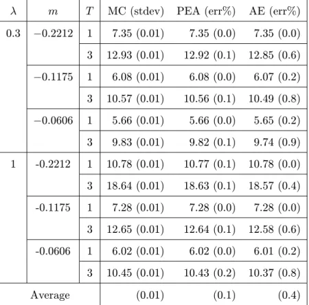
volatility σ, and moneyness. n= 4 and ρij = 0.7. . . 46 3.1 The comparison of basket option prices with MC, AE and CV

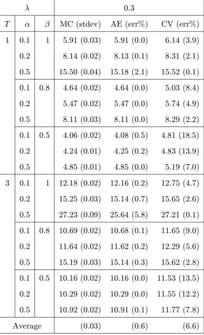
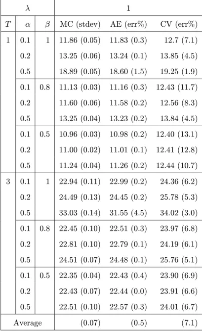
methods. η=−0.08, λ = 0.3. . . 63 3.2 The comparison of basket option prices with MC, AE and CV

methods. η=−0.08, λ = 1. . . 64 3.3 The comparison of basket option prices with MC, AE and CV

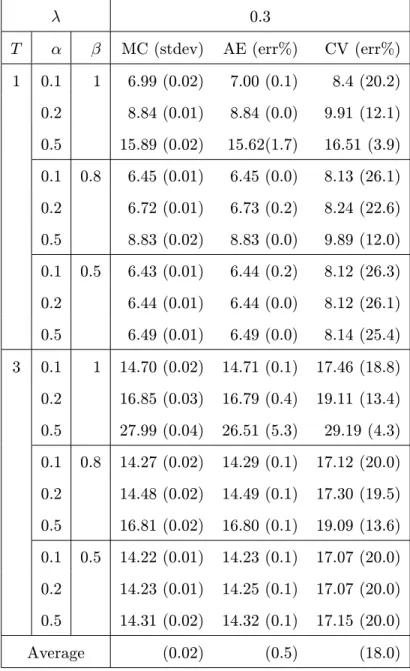
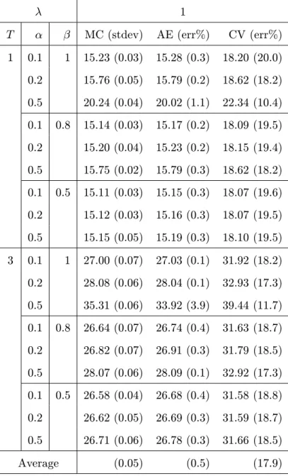
methods. η=−0.3, λ= 0.3. . . 66 3.4 The comparison of basket option prices with MC, AE and CV

methods. η=₋0.3, λ= 1. . . 67 3.5 The comparison of basket option prices with MC, AE and

PEA methods. σi(t, S) = 0.2. . . 68 3.6 The comparison of basket option prices with MC, AE and

PEA methods. σ_i(t, S) = 0.5. . . 70 4.1 The comparison of European basket call option prices with

the MC, AE, and LB methods. λ= 0.3 . . . 87 9

(10)

4.3 The comparison of European basket call option prices with the MC, AE, and LB methods in local volatility models. . . . 90 4.4 The comparison of basket option prices with MC, PEA, AE

and LB methods. σi(t, S) = 0.2. . . 91 4.5 The comparison of basket option prices with MC, PEA, AE

and LB methods. σi(t, S) = 0.5. . . 93

(11)

Some of the research presented in this thesis can also be found in the following publications:

1. Xu, G. and Zheng, H. (2009), Approximate basket options valuation for a jump-diffusion model. Insurance: Mathematics and Economics, 45, 188-194,

which has the abstract:

“In this paper we discuss the approximate basket options valuation for a jump-diffusion model. The underlying asset prices follow some correlated diffusion processes with idiosyncratic and systematic jumps. We suggest a new approximate pricing formula which is the weighted sum of Rogers and Shi’s lower bound and the conditional second mo-ment adjustmo-ments. We show the approximate value is always within the lower and upper bounds of the option and is very sharp in our nu-merical tests.”

2. Xu, G. and Zheng, H. (2010), Basket options valuation for a local volatility jump-diffusion model with the asymptotic expansion method. Insurance: Mathematics and Economics, 47, 415-422,

which has the abstract:

“In this paper we discuss the basket options valuation for a jump-diffusion model. The underlying asset prices follow some correlated local volatility diffusion processes with systematic jumps. We derive a forward partial integro-differential equation (PIDE) for general stochas-tic processes and use the asymptostochas-tic expansion method to approximate the conditional expectation of the stochastic variance associated with the basket value process. The numerical tests show that the suggested method is fast and accurate in comparison with the Monte Carlo and other methods in most cases.”

(12)

(13)

Introduction

A basket option is an exotic option whose payoff depends on the value of a portfolio of assets. The components in an equity basket can be single stocks, equity indices or funds. Basket options are widely used in portfolio risk management as they are flexible to build and allow risk managers or traders to hedge their risks with one single product. Basket options can also be part of complex trading strategies, like dispersion trading. The cost associated with buying a basket option is lower than the cost of buying a portfolio of separate options written on each of the basket’s components.

Basket options are in general difficult to price and hedge due to the lack of analytic characterization of the distribution of a weighted sum of correlated underlying assets. In order to show the difficulty of the pricing and also the motivation for this thesis, we first consider the basket option pricing problem in the Black-Scholes model. Assume a basket is composed of n assets, and the underlying asset prices are S1, . . . , Sn. The basket value at timet is given

by S(t) = n X i=1 wiSi(t),

where wi are positive constant weights. The payoff of a basket call option is then given by S(T)₋K + , 13

(14)

where K is the strike price and T is the maturity of the option. The basket call option price at time 0 is given by

e−rTE[(S(T)₋K)+]

whereris the risk-free interest rate, and Erisk-neutral expectation operator. In the Black-Scholes model, the underlying assets S_i are assumed to follow the geometric Brownian motions

dSi(t)

Si(t) =rdt+σidWi(t),

whereσi are constant volatilities, andWi are Brownian motions with correla-tion matrix (ρij). Then the basket price is the weighted sum of the correlated log-normal random variables and can be written as

S(t) = n X i=1 wiSi(0)e(r− 1 2σ2i)t+σiWi(t)_.

S(t) is no longer a lognormal random variable and the exact distribution is not known. It is not possible to derive a closed-form solution of the basket option price. The exact same problem occurs when pricing an arithmetic Asian option, whose price depends on the arithmetic average underlying price over discrete time points.

There are several methods to price the basket options in the literature. They can be roughly divided into three categories as follows: numerical meth-ods, lower and upper bounds, and analytic approximations. The numerical methods include Monte Carlo simulations, partial (integro-) differential equa-tions based approaches, tree methods and fast Fourier transform methods. See Lord (2006) and Dionne et al. (2006) for details. The Monte Carlo sim-ulation is the most flexible method, which allows us to choose more realistic models and to price products with high number of asset dimensions. It is also very accurate but very time-consuming. For other numerical methods, the major issue is asset dimensionality. When the number of dimensions is high (above ten), they become impractical to use, as the number of the state

(15)

variables may be too large, see Ju (2002), Leentvaar (2008) and Hepperger (2010). When pricing basket options with high number of asset dimensions, the numerical methods may be too slow for practical purposes, and it is very natural to look to analytical approximations or pricing bounds.

The analytical approximations are normally only available for basket op-tions when the underlying assets have analytical soluop-tions, as they depend essentially on the analytically known distributions and moments of the assets. Most work in the literature for analytical approximations assumes that un-derlying asset prices follow geometric Brownian motions. The basket value is then the sum of correlated lognormal variables. The main idea of the analytic approximation method is to find a simple random variable to approximate the basket value and then to use it to get a closed-form pricing formula. This approximate random variable is required to match some moments of the basket value. One of the most used analytical approximations is Levy’s lognormal moment matching method. Levy (1992) uses a lognormal variable to approximate the sum of the correlated lognormal variables and match the first two moments. Analytical approximations can be very useful to quickly generate a reasonably accurate estimate of the option value and its sensi-tivities. In risk management, financial practitioners generally prefer to use an analytical approximation at an acceptable level of accuracy rather than a more accurate but computationally complicated method. For example, in counterparty credit risk management, exposure calculations for the basket option require to price the option at each point out into the future to the maturity of the option. In order to get the potential future exposure, the option may need to be priced thousands of times. In this case, the analytical closed-form approximation is highly desirable.

Bounds can be good approximations if they are tight enough. The lower and upper bounds are developed in two settings: model dependent bounds and model independent bounds. Model independent bounds are robust and can sometimes be associated with static sub-replicating and super-replicating strategies for basket options, see Hobson et al. (2005a, 2005b). However,

(16)

these bounds are way too weak and can not be used to quote option prices. In the model dependent setting, Curran (1994) and Rogers and Shi (1995) use conditioning and Jensen’s inequality to derive a lower bound in the Black-Scholes model. This bound is generally very tight and is one of the most accurate approximations for basket option prices. We call this bound Rogers and Shi’s lower bound. Because Rogers and Shi’s lower bound depends cru-cially on the conditioning variable which is derived from the estimation of the basket value and the closed-form solutions of individual asset prices, it is challenging to extend it to more realistic models, see Albrecher et al. (2008). Upper bounds are normally less tight than lower bounds. Rogers and Shi (1995) propose an upper bound by estimating the error of the lower bound. The comonotonicity approach introduced by Dhaene et al. (2002a, 2002b) can also be used to derive lower and upper bounds for basket options. See a very good recent survey by Deelstra et al. (2010) for recent developments in pricing bounds.

Although most work in the literature assumes that underlying asset prices follow geometric Brownian motions, it can be argued that the Black-Scholes model is inconsistent with options data in the market, see Andreasen (2000) and Cont and Tankov (2004), as it is not able to capture the volatility smile or skew. To equate the Black- Scholes formula with quoted prices of European calls and puts, it is generally necessary to use different volatilities (so-called implied volatilities) for different option strikes and maturities. Merton (1976) introduces the jump-diffusion model by adding Poisson jumps to the Black-Scholes diffusion model. The importance of a jump component has been discussed in Cont and Tankov (2004). Dupire (1994) keeps the diffusion framework of the Black-Scholes model and introduces the local volatility model by allowing the volatility to be a deterministic function of time and the asset price. The local volatility model retains the market completeness of the Black-Scholes model. Andersen and Andreasen (2000) introduce the local volatility jump-diffusion model as a generalization of both the Merton model and the local volatility model, by adding the Poisson jump to the

(17)

local volatility dynamic. The jump-diffusion models are able to generate volatility skew and smiles, see Andreasen (2000) and Cont and Tankov (2004) for detail discussions of jump-diffusion models and other extensions of the Black-Scholes model in the literature.

In this thesis, we focus on the pricing of basket options in jump-diffusion models. We propose three new approximate pricing methods for the jump-diffusion models. The first method is the partial exact approximation (PEA) which is the weighted sum of Rogers and Shi’s lower bound and the condi-tional second moment adjustments. The second one is based on the partial integral differential equation (PIDE) method and the asymptotic expansion method. We reduce a multidimensional local volatility jump-diffusion model problem to a one-dimensional stochastic volatility jump-diffusion model, then derive a forward PIDE for the basket options price with an unknown condi-tional expectation, or local volatility function, and finally apply the asymp-totic expansion method to approximate the local volatility function. The third one is the lower bound approximation which applies the asymptotic ex-pansion method to the basket price and then approximates the Rogers and Shi’s lower bound.

The thesis consists of five chapters. The material in Chapter 2 and Chap-ter 3 is based on Xu and Zheng (2009, 2010). In ChapChap-ter 2, the underlying as-set prices follow some jump-diffusion models with constant volatilities. Apart from correlated Brownian motions, there are two types of Poisson jumps: a systematic jump which affects all asset prices and idiosyncratic jumps which only affect specific asset prices. We derive closed-from expressions for lower and upper bounds. We also propose a partial exact approximation which is the weighted sum of Rogers and Shi’s lower bound and the conditional second moment adjustment and is guaranteed to lie in between the lower and the upper bound. The numerical tests show that the approximation is very tight. In Chapter 3, the underlying asset prices follow some correlated local volatil-ity diffusion processes with systematic jumps. We derive a forward PIDE for general stochastic processes and use the asymptotic expansion method to

(18)

ap-proximate the conditional expectation of the stochastic variance associated with the basket value process. The numerical tests show that the suggested method is fast and accurate in comparison with the Monte Carlo and other methods in most cases. In Chapter 4, we derive an approximation of Rogers and Shi’s lower bound to the basket options pricing for local volatility jump-diffusion models. We expand the asset prices to the second order using the asymptotic expansion method and obtain an easily implemented and fast to compute lower bound approximation. If the local volatility function is time independent, then there is a closed-form expression for the approximation. Numerical tests show that our lower bound approximation is very fast and performs very well in most cases in comparison with the Monte Carlo method and the approximation methods proposed in Chapter 2 and 3. In Chapter 5, we describe our conclusions and provide some suggestions for potential future research in this field.

(19)

Partial Exact Approximation

2.1 Introduction

In this chapter we will discuss the approximate basket options valuation for a jump-diffusion model. The underlying asset prices follow some correlated diffusion processes with idiosyncratic and systematic Poisson jumps. Monte Carlo simulation is a suitable numerical method to valuate basket options for this model. It is simple and accurate but is also very time-consuming. The other numerical methods may be impractical to use. We will focus on deriving accurate and easy to implement bounds and analytical approximations in this chapter.

Most work for basket options pricing in the literature assumes that un-derlying asset prices follow geometric Brownian motions. The basket value is then the sum of correlated lognormal variables. The main idea of the analytic approximation method is to find a simple random variable to approximate the basket value and then to use it to get a closed-form pricing formula for the basket option. The approximate random variable is required to match some moments of the basket value. Levy (1992) uses a lognormal variable, Posner and Milevsky (1998) use a shifted lognormal variable, and Milevsky and Posner (1998) use a reciprocal gamma variable. Gentle (1993) approx-imates the arithmetic average in the basket payoff by a geometric average,

(20)

and Ju (2002) uses Taylor expansion and matches the first two moments. See Krekel et al. (2004) for the performance comparisons of these methods in the Black-Scholes model. The Edgeworth expansion introduced by Jarrow and Rudd (1982) is also widely used. The main drawback of these approximations is that the error can only be estimated by numerical analysis.

Curran (1994) introduces the idea of conditioning variable and condi-tional moment matching. The option price is decomposed into two parts: one can be calculated exactly and the other approximately by conditional moment matching method. The conditioning approach can also be used to find the bounds of the basket option. Rogers and Shi (1995) derive the lower and upper bounds, Nielsen and Sandmann (2003) improve the upper bound. Dhaene et al. (2002a, 2002b) introduce the concept of comonotonicity and discuss the comonotonic lower and upper bounds, Vyncke et al. (2004) propose a two moment matching approximation with a convex combination of the comonotonic lower and upper bounds for Asian options, Deelstra et al. (2004) suggest a similar approximation for basket options. See Deelstra et al. (2004) and Lord (2006) for further extensions and applications.

All the work mentioned above assumes a diffusion asset price model. Ef-forts have been made to extend to more general asset price models. Albrecher and Predota (2002, 2004) discuss variance-gamma and NIG L´evy processes, while Flamouris and Giamouridis (2007) extend the framework to a Bernoulli jump-diffusion model. For these three models, the distributions for the un-derlying assets are available, and so the moment matching method is used to derive the analytical approximations. Albrecher et al. (2005) discuss upper bound in L´evy models. Hobson et al. (2005a) and Chen et al. (2008) discuss model free upper bounds. Hobson et al. (2005b) find model free lower bounds for basket options on exactly two underlying assets. Albrecher et al. (2008) derived model free lower bounds for Arithmetic Asian options via European call options on the same underlying that are assumed to be observable in the market. See a good recent survey by Deelstra et al. (2010) for recent developments in the pricing bounds.

(21)

In this chapter we assume the underlying asset prices follow jump-diffusion models with constant volatilities and two types of Poisson jumps: a system-atic jump which affects all asset prices and idiosyncrsystem-atic jumps which only affect specific asset prices. In correlation modelling this is a type of Marchall-Olkin exponential copulas. Since the basket value is no longer the sum of lognormal variables it is not clear what conditioning random variables one should use to approximate the basket value. The main contribution of this chapter is that we derive a new approximation to the basket call option price. This approximation is a weighted sum of the lower bound and the conditional second moment adjustments and is guaranteed to lie in between the lower bound and the upper bound. The numerical tests show that the approximation is very tight in comparison with the Monte Carlo results.

This chapter is organized as follows. Section 2.2 formulates the jump-diffusion asset price model and reviews some results on approximation and bounds in diffusion asset price models. Section 2.3 discusses conditioning random variables and derives closed-form expressions for the lower and up-per bounds. Section 2.4 derives a new approximation formula for basket options and shows it is bounded. Section 2.5 elaborates on the numerical implementation and provides some numerical tests. Section 2.6 is the sum-mary.

2.2 Model Formulation and Literature

Re-view

Assume (Ω, P,_F,(_Ft)0≤t≤T) is a filtered risk-neutral probability space and

Ft is the augmented natural filtration generated by correlated Brownian mo-tions W1, . . . , Wn with correlation matrix (ρij)ni,j=1 and independent Poisson

processes N0, . . . , Nn with intensities λ0. . . , λn. Assume also that

Brown-ian motions and Poisson processes are mutually independent. Assume the portfolio is composed of n assets and the asset prices S1, . . . , Sn satisfy the

(22)

stochastic differential equations dSi(t)

Si(t)

=ridt+σidWi(t) +h0id[N0(t)−λ0t] +h1id[Ni(t)−λit], (2.1) for i = 1, . . . , n, where ri =r−δi and r is the risk-free interest rate and δi are the continuous dividend yields of assets i, σ_i are volatilities of assets i, and h0

i, h1i are percentage jump sizes of assets i at time of jumps of Poisson processesN0andNi, respectively. All coefficients are assumed to be constant.

Solutions to equations (2.1) are given by Si(t) = Si(0)e(ri− 1 2σi2−h0iλ0−hi1λi)t+σiWi(t) Y 0≤s≤t (1 +h0_iΔN0(s) +h1iΔNi(s)) = S_i(0)e(ri−12σi2−h0iλ0−h1iλi)t+σiWi(t)+Ci0N0(t)+Ci1Ni(t)_, where C0

i = ln(1 +h0i) and Ci1 = ln(1 +h1i). The second equality is due to the fact that independent Poisson processes never jump simultaneously, see Lando (2004).

Almost all the research in the literature on basket options pricing assumes that asset prices Si follow geometric Brownian motions (corresponding to h0

i =h1i = 0 for alli), which cannot explain asset prices jumps for unexpected market events. The asset price dynamics (2.1) incorporates both systematic events and idiosyncratic events. More precisely, if an unexpected market event N0 occurs at time t then all underlying asset prices Si(t) have jumps

of percentage sizes h0

i for i = 1, . . . , n, on the other hand, if an unexpected eventNioccurs at timet, then only asset priceSi(t) has a jump of percentage size h1

i but all other asset prices are not affected. In between jumps asset prices are driven by diffusion processes.

The basket value at time t is given by S(t) =

n

X

i=1

wiSi(t)

wherewi are positive constant weights. The basket call option price at time 0 is given by

(23)

where K is exercise price, T maturity time, and E risk-neutral expectation operator. The exercise time T is fixed as we only deal with European style options. To simplify the notation we will omit T from now on in this chapter, for example, we write Wi instead of Wi(T). The basket value at time T can be written as S = n X i=1 aieσiWi+C 0 iN0+Ci1Ni _(2.2) where a_i = w_iS_i(0)e(ri−1₂σi2−h0iλ0−h1iλi)T_, _W

i are normal variables with mean 0 and variance T, and Ni are Poisson variables with parameters λiT, i = 1, . . . , n.

Almost all work in the literature on Asian or basket options pricing as-sume the underlying asset prices follow lognormal processes, which corre-sponds to h0

i = h1i = 0 for all i in our model setup. Since the analytical approximations and bounds for Asian options can be relatively straightfor-ward to adapt to basket options, and vice versa, we do not differentiate these two types of options, even though some techniques are originally developed for Asian options. We now review some well-known approaches in approxi-mation and error bound estiapproxi-mation for the pure diffusion case.

Levy (1992) approximates the basket value S with a lognormal variable which has the same first two moments as those of S and derives the approx-imate closed-form pricing formula for C0. We briefly outline this method as

it is probably the most frequently used method in practice. Assume the first two moments of S are M and V2_{, and} _Y _{is a normal variable with mean} _m

and variancev2_{. Matching the first two moments of} _S _{with those of}_eY _yields m = 2 log(M)−1

2log(V

2₎

v2 = log(V2)−2 log(M), then the basket call option price can be approximated by

C0 ≈ e−rT[MΦ(d1)−KΦ(d2)] (2.3)

with

d1 =

m+v2₋_ln_K

(24)

Φ(_∙) is the cumulative distribution function of a standard normal random variable. We implement this method in our numerical tests. Posner and Milevsky (1998) extend this approach to a shifted lognormal variable which matches the first four moments of S. The results are very good when matu-rityT and volatilitiesσiare relatively small. The performance deteriorates as T or σi increases. Milevsky and Posner (1998) use a reciprocal gamma vari-able to approximate the basket value S and match the first two moments. The motivation is that the distribution of sums of correlated log-normally distributed random variables converges to the reciprocal gamma distribu-tion under some parameter restricdistribu-tions. Let GR be the reciprocal gamma distribution and G the gamma distribution with parameters α, β, then by definition GR(y, α, β)=1 ₋G(1

y, α, β). Assume the first two moments of S are M and V2_{, and the random variable} _Y _{is reciprocal gamma distributed.}

Matching the first two moments of S with those of eY _yields α= 2V 2₋_M2 V2₋_M2 β = V 2₋_M2 M V2 ,

and the approximate basket option price has a closed-form expression which is similar to the Black-Scholes formula:

C0 ≈ e−rT[M G(

1

K, α−1, β)−KG( 1

K, α, β)]. (2.4) Ju (2002) uses Taylor expansion around zero volatilities to approximate the ratio of the characteristic function of the basket price to that of the approx-imating lognormal variable. The volatilities are scaled by a parameter z and then one applies a Taylor expansion to the ratio with respect to z around z = 0. This method is similar in spirit to the asymptotic expansion used in Chapter 3, see Benhamou et al. (2009). The ratio is expanded up to the sixth order in the approximation.

The drawback of these moment matching approximations is that the ap-proximation error can only be estimated by numerical analysis.

(25)

Curran (1994) introduces the idea of conditioning random variables. As-sume Λ is a random variable which has strong correlation with Sand satisfies S _≥K whenever Λ≥dΛ for some constantdΛ. The basket option price can

be decomposed as

E[(S−K)+] = E[(S−K)1[Λ≥dΛ]] +E[(S−K)

+₁

[Λ<dΛ]]. (2.5)

Note that Λ < dΛ does not necessarily imply S < K. Curran (1994) chooses

Λ a normal variable (geometric average Qn_i₌₁Swi

i ) and finds the closed-form expression for the the first part and uses the lognormal variable and the conditional moment matching technique (at the point of strike price K) to find the approximate value of the second part. Deelstra et al. (2004) extend the conditional moment matching approach further by finding a lognormal variable ˜S such that

E[ ˜S_|Λ =λ] =E[S|Λ =λ] and Var( ˜S_|Λ =λ) = Var(S|Λ =λ) for all λ < d_Λ.

Rogers and Shi (1995) use the conditioning variable Λ and Jensen’s in-equality to derive the lower bound of E[(S−K)+_{] as}

E[(S−K)+] = EE[(S−K)+]|Λ≥E(E[S|Λ]−K)+.

The lower bound works very well because the conditioning random variable Λ and the basket value S has a very strong correlation. Curran (1994) derives the same lower bound and uses it to approximate the basket option price. The lower bound can be calculated analytically.

However, by replacing S with its projection on the conditional random variable Λ, there is a projection error between the lower bound and the exact basket option value. Rogers and Shi (1995) derive a strike price independent upper bound ofE[(S−K)+_{] by estimating this error. Nielsen and Sandmann}

(2003) sharpen Rogers and Shi’s upper bound to make it depend on the strike price. The upper bound is expressed as

E(E[S|Λ]−K)++ 1 2E var(S|Λ)1[Λ<dΛ] 1 2 _E[1 [Λ<dΛ]] 1 2.

(26)

where H¨older’s inequality has been applied in the last inequality, see Nielsen and Sandmann (2003) and Rogers and Shi (1995).

Lord (2006) shows the conditional moment matching approximation of Deelstra et al. (2004) lies in between the lower and upper bounds and intro-duces the class of partially exact and bounded approximations.

The only work we are aware of on the jump-diffusion asset price model is the one by Flamouris and Giamouridis (2007). The underlying asset follows a simplified version of the Merton (1976) jump-diffusion model. The jump part is a Bernoulli variable instead of a Poisson variable, which means that there can be maximum of one jump for each asset price during the life of the contract. The basket contains two assets and the two independent Bernoulli variables are used as conditioning variables. With this simplified setup the authors approximate basket value with a lognormal variable under each of the four cases (one may or may not jump and there is a combination of four cases) and approximate the basket option value by the weighted sum of the four approximating values. Even for Bernoulli jumps, this method may not work when the number of the underlying assets is large. If there are n underlying assets, then n conditioning variables are needed, and the basket option value is the weighted sum of 2n _{terms. This method does not work} for Poisson jumps as the number of terms would be too large to manage.

For the jump-diffusion asset price models (2.1), there are many open questions to be answered. For example, how should one choose the

(27)

condi-tioning variable? Are there closed-form expressions for the lower and upper bounds? Is the approximation guaranteed to lie in between the lower and upper bounds? How accurate and fast is the computation? etc. We will address these questions in the rest of the chapter.

2.3 Exact Part and Bounds of Basket

Op-tions

To derive bounds and use the conditioning variable approach to approximate the basket option price for a jump-diffusion asset price model, we need first to decide what conditioning variables to use. We want to put as much infor-mation about S as possible in the conditioning variables. In the literature a normal variable is usually chosen as the conditioning variable, see Deelstra et al. (2004) and Vanduffel et al. (2008), but it is not clear what one should choose for a jump-diffusion asset price model. From (2.2) we have

S _≥ n X i=1 ai(1 +σiWi+Ci0N0+Ci1Ni) (2.6) ≥ c+m0N0+m2N +σW

where c = Pn_i₌₁ai, m0 = Pn_i₌₁aiCi0, m2 = min1≤i≤n(aiCi1), and σ2 =

Pn i=1

Pn

j=1aiajρijσiσjT are constant, and N0 and N =

Pn

i=1Ni are

Pois-son variables with parameters λ₀T and λT = Pn_i₌₁λ_iT, respectively, and W = _σ1 Pn_i₌₁aiσiWi is a standard normal variable. Note that N0, N and

W are independent to each other. We used the Taylor expansion for the inequality in (2.6).

If we chooseX = (N0, N, W) and define φ(X) =m0N0+m2N+σW and

dX = K −c then we have S ≥ K whenever φ(X) ≥ dX. Therefore X can be a conditioning variable. The motivation for this choice is that we want to extract as much information as possible from normal variables and Poisson variables. The reason we choose two Poisson variables N0 and N instead

(28)

greater impact on basket value S than any individual shock N_i. This gives much better approximation with minimal increase of computation load.

2.3.1 Exact Part of Basket Options

The basket option price can be decomposed into two parts via conditioning as in (2.5), and the first part can be calculated explicitly when the underlying asset prices follow geometric Brownian motions. For the jump-diffusion asset price model (2.1), we can also find the closed-form expression for the exact part E[(S₋K)1[φ(X)≥dX]]. The exact part will appear in the approximation

formula (2.25) for the basket option in next section.

We need first to find the conditional expectation of the basket value S given the conditioning variable X = (N0, N, W) = (n0, k, y).

E[S|X = (n0, k, y)] = n X i=1 aiE[eCi0N0+Ci1Ni+σiWi_|_X _{= (n} 0, k, y)] = n X i=1 aiE[eCi0N0_|_N 0 =n0]E[eC 1 iNi_|_N ₌_k]E[eσiWi_|_W ₌_y].

Here we have used the independence of N0, N, W. For N =Pni=1Ni define ˉ

Ni =N −Ni, then ˉNi is a Poisson variable with parameter

ˉ

λiT := (λ−λi)T and is independent of Ni. From

P(Ni =ki|N =k) = P(Ni =ki,Nˉi =k−ki) P(N =k) = P(Ni =ki)P( ˉNi =k−ki) P(N =k) = k! ki!(k−ki)!( λi λ) ki₍λˉi λ) k−ki

(29)

we get E[eCi1Ni_|_N ₌_{k] =} k X ki=0 eCi1ki k! ki!(k−ki)!( λi λ) ki₍λˉi λ) k−ki = eCi1λi λ + ˉ λ_i λ k .

Note that (Ni = ki|N = k) is a binomial random variable and we can easily get its mean, variance and the moment generating function. With-out this, we can not proceed further to get closed-form expressions. For W = 1

σ

Pn

i=1aiσiWi, Deelstra et al. [2004] show that E[eσiWi_|_W ₌_{y] =}_e1₂(σ2iT−R2i)+Riy where R_i = 1 σ Pn j=1ajρijσiσjT. Therefore E[S_|X = (n0, k, y)] = n X i=1 Ai(n0, k, y) and Ai(n0, k, y) =aie 1 2(σ2iT−R2i)eCi0n0 eCi1λi λ + ˉ λ_i λ k eRiy_. _(2.7)

We can now easily find the exact part of the basket option value. E[(S₋K)1[φ(X)≥dX]] = E[E[S_|X]1[φ(X)≥dX]]−KP(φ(X)≥dX) = ∞ X n0=0 ∞ X k=0 P(N0 =n0)P(N =k) Z ∞ dX−m₀n₀−m₂k σ n X i=1 Ai(n0, k, y)dΦ(y) −KP(φ(X)≥dX)

(30)

above equation becomes ∞ X n0=0 ∞ X k=0 P(n0, k) n X i=1 aie 1 2σ2iTeCi0n0 eC1iλi λ + ˉ λi λ k Φ (Ri−z(n0, k)) −K ∞ X n0=0 ∞ X k=0 P(n0, k)Φ (−z(n0, k)) = ∞ X n0=0 ∞ X k=0 P(n0, k) n X i=1 ˜ Si(n0, k)Φ(Ri−z(n0, k))−KΦ(−z(n0, k)) ! (2.8) where Φ(y) is the cumulative distribution function of the standard normal random variable y and

˜ Si(n0, k) = aie 1 2σi2TeCi0n0 eCi1λi λ + ˉ λi λ k . (2.9)

Note that (2.8) involves the summation of an infinite series. But we only need a small number of terms to get accurate results, because P(n0, k) converges

to zero very quickly.

2.3.2 Bounds for Basket Options Prices

The method of finding the lower and upper bounds of basket option price in Rogers and Shi (1995) and Nielsen and Sandmann (2003) works for the jump-diffusion asset price model (2.1) by conditioning on_{φ(X)_≥dX}. This leads to LB ≤E[(S−K)+]≤UB where LB = E(E[S|X]−K)+ (2.10) UB = LB + 1 2E Var(S|X)1[φ(X)<dX] 1 2 _E[1 [φ(X)<dX]] 1 2. (2.11)

(31)

Lower Bound

We will derive the closed-form lower bound LB in (2.10) below. E(E[S|X]−K)+ = ∞ X n0=0 ∞ X k=0 P(n0, k) Z ∞ −∞ " _n X i=1 Ai(n0, k, y)−K #+ dΦ(y) For fixed n0 and k we need to compute the integral

Z ∞ −∞ " _n X i=1 Ai(n0, k, y)−K #+ dΦ(y), (2.12) where Ai(n0, k, y) is defined in (2.7). To avoid the numerical integration we

do the following: for fixed n0, k, define a convex function

f(y) = n

X

i=1

Ai(n0, k, y)−K.

IfRi 6= 0 at least for somei, thenf(y) is a strictly convex function. We want to find y∗ ₌_y(n

0, k) such that f(y∗) = 0. There are four cases to consider.

1. Ri = 0 for all i. Then f is a constant. The integral of (2.12) is a constant and equals

" _n X i=1 e Si(n0, k)−K #+ . Note that Sei(n0, k) is defined in (2.9).

2. Ri ≥ 0 for all i and Ri > 0 for at least one i. Then f is strictly increasing and f(_−∞) = ₋K and f(_∞) = _∞, which implies that there is a unique root y∗ _for _f_{(y). We only need one numerical search}

to avoid the numerical integration. The integral of (2.12) has a closed-form on interval [y∗,_∞) and equals

Z ∞ y∗ " _n X i=1 Ai(n0, k, y)−K # dΦ(y) = n X i=1 e Si(n0, k)Φ(Ri−y∗)−KΦ(−y∗).

(32)

3. R_i _≤ 0 for all i and R_i < 0 for at least one i. Then f is strictly decreasing and f(−∞) = ∞ and f(∞) = −K. which implies that there is a unique root y∗ for f(y). The integral of (2.12) has a closed-form on interval (−∞, y∗_{] and equals}

Z y∗ −∞ " _n X i=1 Ai(n0, k, y)−K # dΦ(y) = n X i=1 e

Si(n0, k)Φ(y∗−Ri)−KΦ(y∗).

4. Ri > 0 for at least one i and Ri < 0 for at least another i. Then f is U-shaped with f(_−∞) = f(_∞) = _∞. There is unique minimum point ymin for f(y). If f(ymin) ≥ 0, then the integral of (2.12) has a closed-form on interval (−∞,_∞) and equals

Z ∞ −∞ " _n X i=1 Ai(n0, k, y)−K # dΦ(y) = n X i=1 e Si(n0, k)−K.

If f(ymin) < 0, then there are two roots y₋∗ and y₊∗ (y₋∗ < y₊∗) for f(y). The integral of (2.12) is the sum of two closed-forms on intervals (−∞, y₋∗] and [y₊∗,_∞) and equals

Z y∗ − −∞ " _n X i=1 A_i(n0, k, y)−K # + Z ∞ y∗ + " _n X i=1 A_i(n0, k, y)−K # dΦ(y) = n X i=1 e Si(n0, k) Φ(y₋∗ −Ri) + Φ(Ri−y+∗) −K Φ(y₋∗) + Φ(₋y₊∗).

We have derived a closed-form expression for the lower bound of the jump-diffusion asset price model. We may use a numerical search algorithm such as the Newton method or the bisection method to find the root off and then get the closed-form value of the integration. Lord (2006) has a similar discussion concerning the number of roots of the function f when the underlying assets are lognormally distributed.

(33)

Upper Bound

We will derive a closed-form and computable expression for UB in (2.11), which is tedious but straightforward. We have already derived the lower bound and so we only need to derive the error term. We start withE[1[φ(X)<dX]]

and we have E[1[φ(X)<dX]] = ∞ X n0=0 ∞ X k=0 P(n0, k)Φ(z(n0, k)). (2.13)

Note that z(n0, k) = dX−m0_σn0−m2k. We also have

E[Var(S_|X)1[φ(X)<dX]] =E[(E[S

2

|X]₋(E[S_|X])2)1[φ(X)<dX]]. (2.14)

We need to find the two terms on the right hand sight of (2.14). The second term can be written as

E[(E[S_|X])21[φ(X)<dX]] = ∞ X n0=0 ∞ X k=0 P(n0, k) Z z(n0,k) −∞ n X i=1 Ai(n0, k, y) !2 dΦ(y) = ∞ X n0=0 ∞ X k=0 P(n0, k) ∙ n X i=1 n X j=1 ˜ Si(n0, k) ˜Sj(n0, k)eRiRjΦ(z(n0, k)−Ri−Rj) ! .(2.15)

The first term of the right hand sight of (2.14) can be expressed as E[E[S2_|X]1[φ(X)<dX]] = X i6=j aiajE[E[e(C 0 i+Cj0)N0+(Ci1Ni+Cj1Nj)+(σiWi+σjWj)_|_X]1 [φ(X)<dX]] + n X i=1 a2_iE[E[e2Ci0N0+2Ci1Ni+2σiWi_|_X]1 [φ(X)<dX]] (2.16)

(34)

The second term of the right hand sight of (2.16) can be easily written as n X i=1 a2 i ∞ X n0=0 ∞ X k=0 P(n0, k)e2C 0 in0(e2Ci1λi λ + ˉ λ_i λ) k_e2(σ2 iT−R2i) Z z(n0,k) −∞ e2Riy_dΦ(y) = ∞ X n0=0 ∞ X k=0 P(n0, k) n X i=1 a2_ie2σi2Te2Ci0n0_(e2Ci1λi λ + ˉ λi λ) k_Φ(z(n 0, k)−2Ri) ! (2.17)

It is slightly more involved to find the first term of the right hand sight of (2.16). We first find the conditional expectation of

e(Ci0+Cj0)N0+(Ci1Ni+Cj1Nj)+(σiWi+σjWj)

given the conditioning variable X = (N0, Ni,Nˉi, W) = (n0, ni, k, y) and ˉNi = N ₋N_i. E[e(Ci0+Cj0)N0+(Ci1Ni+Cj1Nj)+(σiWi+σjWj)_|_X _{= (n} 0, ni, k, y)] = E[e(Ci0+Cj0)N0_|_N 0 =n0]E[eC 1 iNi_|_N i =ni]E[eC 1 jNj_|_Nˉ i =k] ∙E[e(σiWi+σjWj)_|_W ₌_y] = e(Ci0+Cj0)n0_eC1ini eCj1λj ˉ λi + 1− λ_ˉj λi k eRijσijy+1₂(σ2ijT−R2ijσij2), since E[eCj1Nj_|_Nˉ i =k] = eCj1λj ˉ λi + 1− λ_ˉj λi k

and Deelstra et al. [2004] show that

(35)

where σ2

ij =σi2+σj2+ 2σiσjρij and Rij = Ri_σ+_ijRj. Therefore, the first term of the right hand sight of (2.16) can be written as

X i6=j aiaj ∞ X n0=0 ∞ X ni=0 ∞ X k=0 P(N0 =n0)P(Ni =ni)P( ˉNi =k)e(C 0 i+Cj0)n0+Ci1ni ∙ eC1jλj ˉ λi + 1₋ λ_ˉj λi kZ z(n0,ni,k) −∞ eRijσijy+1₂(σij2T−R2ijσ2ij)Φ(y) = X i6=j aiaj ∞ X n0=0 ∞ X ni=0 ∞ X k=0 P(N0 =n0)P(Ni =ni)P( ˉNi =k)e 1 2σ2ijT ∙ e(C0i+Cj0)n0+Ci1ni eCj1λj ˉ λ_i + 1− λ_j ˉ λ_i k Φ (z(n0, ni, k)−Ri−Rj) !

where z(n0, ni, k) = dX−m0n0−_σm2ni−m2k. We have got every term we need for the upper bound in (2.11).

Note that if we set the jump sizesh0

i andh1i to 0, then our exact part and bounds reduce to the results in the Black-Scholes setting, see Deelstra et al. (2004).

We have conducted some numerical tests for the lower and upper bounds of the jump-diffusion asset price process (see Section 2.5). The results show that the lower bound is in general very tight whereas the upper bound is not sharp and can have large deviations from the true value.

2.4 Partial Exact Approximation of Basket

Options

Denote bySX ₌_E[S_|_{X] the conditional expectation of} _S_given_{X. The error} between the lower bound and the exact basket option value is given by

E[(S−K)+]−LB

= E[(S₋K)+1[φ(X)<dX]]−E[(S

X

(36)

This shows the error is caused by replacingS1[φ(X)<dX] withS

X₁

[φ(X)<dX]. A

simple calculation shows that E[S1[φ(X)<dX]] = E[S X₁ [φ(X)<dX]] (2.18) Var(S1[φ(X)<dX]) = Var(S X₁ [φ(X)<dX]) +E[Var(S|X)1[φ(X)<dX]].(2.19)

Therefore, the lower bound matches the first moment, but not the second moment. If we can find a random variable which matches the first two mo-ments ofS1[φ(X)<dX]then we may reduce the error and improve the accuracy.

We now look for such a random variable and find the properties it must hold. Letε be a random variable independent ofS andX and satisfy the following two equations E[S1[φ(X)<dX]] = E[(S X ₊_ε)1 [φ(X)<dX]] (2.20) Var(S1[φ(X)<dX]) = Var((S X ₊_ε)1 [φ(X)<dX]) (2.21)

From (2.18), (2.20) and the independence of ε and X we get

E[ε] = 0. (2.22)

(2.22) and the independence of ε and X imply Var((SX +ε)1[φ(X)<dX]) = E[(SX +ε)21[φ(X)<dX]]−(E[(S X ₊_ε)1 [φ(X)<dX]]) 2 = E[(SX)21[φ(X)<dX]] +E[ε 2₁ [φ(X)<dX]]−(E[S X₁ [φ(X)<dX]]) 2 = Var(SX1[φ(X)<dX]) +E[ε 2_]E[1 [φ(X)<dX]]. (2.23)

From (2.19), (2.21), and (2.23) we get

E[ε2] = E[Var(S|X)1[φ(X)<dX]]

E[1[φ(X)<dX]]

≡ε2₀. (2.24) We can now present the main result of this chapter.

Theorem 1 Let AC0 =E[(S−K)+1[φ(X)≥dX]] + 3 X i=1 piE[(SX +αi−K)+1[φ(X)<dX]] (2.25)

(37)

where p₁ = 1/6, p₂ = 2/3, p₃ = 1/6, and α₁ =₋√3ε0, α2 = 0, α3 =

√

3ε0.

Then

LB _≤AC0 ≤UB,

where LB and UBare defined in (2.10) and (2.11).

Proof. Letεbe a discrete random variable taking values αi with probabilities pi for i = 1,2,3. Then E[ε] = 0 and E[ε2] = ε20, i.e., ε satisfies (2.22) and

(2.24). We can now show that the new approximation is bounded by the lower and upper bounds. We first derive the upper bound.

E[(SX +ε₋K)+1[φ(X)<dX]] ≤ E[(SX −K)+1[φ(X)<dX]+ε +₁ [φ(X)<dX]] = E[(SX ₋K)+1[φ(X)<dX]] + 1 2E[|ε|]E[1[φ(X)<dX]] ≤ E[(SX ₋K)+1[φ(X)<dX]] + 1 2E[ε 2_]1 2E[1_[_φ₍_X₎_<d X]] = E[(SX ₋K)+1[φ(X)<dX]] + 1 2E[Var(S|X)1[φ(X)<dX]] 1 2E[1_[_φ₍_X₎_<d X]] 1 2.

Since ε is symmetric around 0, i.e., F(x) +F(−x) = 1 where F is the distribution function of ε, we can also estimate the lower bound.

E[(SX ₊_ε₋_K₎+₁ [φ(X)<dX]] = Z ∞ −∞ E[(SX +η₋K)+1[φ(X)<dX]]dF(η) = Z ∞ 0 E[[(SX +η₋K)++ (SX ₋η₋K)+]1[φ(X)<dX]]dF(η) ≥ 2 Z ∞ 0 E[(SX ₋K)+1[φ(X)<dX]]dF(η) = E[(SX −K)+1[φ(X)<dX]] Therefore, LB≤E[(SX +ε₋K)+1[φ(X)<dX]] +E[(S−K) +₁ [φ(X)≥dX]]≤UB.

(38)

We choose e−rT_AC

0 to approximate the basket option value at time 0. It

is clear from the proof that Theorem 1 holds for any random variableεas long as it is symmetric and satisfies (2.22) and (2.24). A normal distribution seems a natural choice, but then one has to deal with a numerical integration. We chooseε to be a discrete random variable taking values ₋√3ε0,0,

√

3ε0 with

probabilities 1/6,2/3,1/6, respectively, which matches the first five moments of a normal variable. We can expect the behaviour of εis similar to that of a normal variable with the added advantage that we do not need to compute the numerical integration. This choice of ε also shows that the lower bound plays a dominant role in the approximation with a weight 2/3, the other two parts with a weight 1/6 each may be explained as the adjustment to the lower bound for the second moment.

Since the basket call option price tends to 0 as strike price K _{→ ∞}, we would expect the approximate price e−rT_AC

0 tends to 0 too. This is indeed

the case as shown in the next result.

Theorem 2 The value AC0 defined in (2.25) tends to 0 as strike price K

tends to infinity.

Proof. The proof is similar to Theorem 4 in Lord (2006). We can write AC0

as AC0 =E[(S−K)+1[φ(X)≥dX]] +E (SX +ε₋K)+1[φ(X)<dX] (2.26) where ε is a discrete random variable defined in Theorem 1. Since the call price tends to 0 asK _{→ ∞}it is obvious that the first term of (2.26) tends to 0 as K _{→ ∞}. We now estimate the second term of (2.26). Let ˉS =SX ₊_ε, then 0 ≤ E( ˉS₋K)+1[φ(X)<dX] ≤E( ˉS₋K)+ = Z ∞ K P( ˉS > x)dx≤ Z ∞ K P(|Sˉ_{| ≥}x)dx ≤ Z ∞ K E[ ˉS2_] x2 dx= E[ ˉS2_] K .

(39)

We only need to show that E[ ˉS2_{] is finite, which then implies} E[ ˉS2_]

K tends to 0 as K _{→ ∞}. SinceSX _and _ε _{are independent and} _{E[ε] = 0 we have}

E[ ˉS2] =E[(SX)2] +E[ε2].

Furthermore, φ(X)≥ dX implies S ≥K, we have P(φ(X)≥ dX)≤ P(S ≥ K), or equivalently,P(φ(X)< dX)≥P(S < K)→1 asK → ∞. Therefore, P(φ(X)< dX)≥1/2 for K sufficiently large. This gives

E[ε2] = E[Var(S|X)1[φ(X)<dX]]

E[1[φ(X)<dX]]

≤2E[Var(S|X)] = 2E[S2]−2E[(SX)2]. Obviously, we have E[ ˉS2_] _≤ _2E[S2_] _< _∞ _for _K _{sufficiently large. We are}

done.

2.5 Implementation and Numerical Tests

The exact part of AC0 has been derived in (2.8). We will find the

approxi-mating part of the basket option value. Denote by α a constant with value

−√3ε0 or 0 or √ 3ε0. Then E[(E[S|X] +α₋K)+1[φ(X)<dX]] = ∞ X n0=0 ∞ X k=0 P(n0, k) Z z(n0,k) −∞ " _n X i=1 A_i(n0, k, y) +α−K #+ dΦ(y). For fixed n0 and k we need to compute the integral

Z z(n0,k) −∞ " _n X i=1 Ai(n0, k, y) +α−K #+ dΦ(y). (2.27) To avoid the numerical integration, we can use considerations similar to those presented in the derivation of the closed-form lower bound. The argument is slightly more involved here because the roots also depend on α. For fixed n0, k, α, define a convex function

ˉ f(y) = n X i=1 Ai(n0, k, y) +α−K.

(40)

ˉ

f(y) is a strictly convex function if R_i ₆= 0 for some i. We want to find y∗ =y(n0, k, α) such that ˉf(y∗) = 0. Four cases may occur.

1. Ri = 0 for all i. Then ˉf is a constant.

2. Ri ≥ 0 for all i and Ri > 0 for at least one i. Then ˉf is strictly increasing and has at most one root.

3. Ri ≤ 0 for all i and Ri < 0 for at least one i. Then ˉf is strictly decreasing and has at most one root.

4. Ri > 0 for at least one i and Ri < 0 for at least another i. Then ˉf is U-shaped and has at most two roots.

To illustrate the point, we assume Ri > 0 for all i. Then ˉf(y) is strictly increasing and ˉf(−∞) = α₋K and ˉf(∞) = ∞. If α _≥ K then ˉf has no root and ˉf(y)>0 for ally. The integral of (2.27) equals

Z z(n0,k) −∞ n X i=1 Ai(n0, k, y) +α−K ! dΦ(y) = n X i=1 ˜ Si(n0, k)Φ(z(n0, k)−Ri) + (α−K)Φ(z(n0, k)).

If α < K then ˉf has a unique root y∗_{, which implies ˉ}_f_(y) _< _{0 for} _{y < y}∗_.

Therefore, if z(n0, k) ≤ y∗ then the integral of (2.27) is 0. If z(n0, k) > y∗

then the integral of (2.27) equals

Z z(n0,k) y∗ n X i=1 Ai(n0, k, y) +α−K ! dΦ(y) = n X i=1 e Si(n0, k) (Φ(z(n0, k)−Ri)−Φ(y∗−Ri)) + (α−K) (Φ(z(n0, k)−Φ(y∗))

which can be computed explicitly. We can similarly discuss and solve all the other cases.

(41)

The only term remains to be computed is ε₀, and ε0 = E[Var(S|X)1[φ(X)<dX]] E[1[φ(X)<dX]] 1 2 .

Since we have found E[1[φ(X)<dX]] in (2.13) and E[Var(S|X)1[φ(X)<dX]] in

(2.14), ε0 can be calculated explicitly.

We do some numerical tests for the European basket call options pricing with the underlying asset price processes (2.1) to evaluate the performance of the partial exact approximation (PEA) and bounds just derived. We consider lognormal approximation (LN) of Levy (1992), recoprocal gamma approximation (RG) of Milevsky and Posner (1998), lower bound, upper bound and PEA method of this chapter for comparisons. The basket call option price approximation formulas for LN and RG methods are given by (2.3) and (2.4).

Table 2.1 lists the results for a heterogeneous portfolio of two assets with different jump intensities (λ0 = 2, λ1 = 1, λ2 = 0.5) and same proportional

jump sizes (h0 = h1 = h2 = −0.2) and volatilities (σ1 = σ2), and with

initial portfolio value S(0) = 100 and correlation coefficient of Brownian motions ρ12= 0.3. We have done the numerical tests for the combination of

the following data: maturity T = 1 and 3, volatility σi = 0.2, 0.5 and 0.8, moneyness is 0.9, 1 and 1.1. (The moneyness is defined by K/E[S(T)], see Deelstra et al. (2004) and Lord (2006) for details.) The number of simulation is 1 million for T = 1 and 3 million forT = 3. Table 2.1 contains 9 columns. The first column reports the option maturity, the second one the volatility, the third one the moneyness, the fourth one the Monte Carlo value with standard deviation in parentheses, the fifth one the partial exact approximate (PEA) value suggested in this chapter, the sixth one the lower bound, the seventh one the upper bound, the eighth one the reciprocal gamma value (Milevsky and Posner (1998)), and the ninth one the lognormal value (Levy (1992)). The total computation time for each case (excluding simulation) takes only a few seconds. Monte Carlo takes much longer to compute but provides the benchmark values.

(42)

Time Vol M’s MC (stdev) PEA LB UB RG LN 1 0.2 0.9 19.49 (0.01) 19.48 19.46 20.09 18.10 18.73 1 14.34 (0.01) 14.34 14.32 15.03 13.36 13.83 1.1 10.28 (0.01) 10.28 10.26 11.04 9.79 10.06 0.5 0.9 25.01 (0.02) 24.97 24.84 26.66 23.00 24.61 1 20.55 (0.02) 20.49 20.36 22.39 18.81 20.03 1.1 16.84 (0.02) 16.76 16.64 18.87 15.43 16.60 0.8 0.9 32.62 (0.02) 32.42 32.05 35.82 28.57 32.49 1 28.77 (0.03) 28.50 28.15 32.34 24.88 28.65 1.1 25.42 (0.03) 25.10 24.77 29.40 21.79 25.33 3 0.2 0.9 28.95 (0.04) 28.98 28.80 32.32 25.51 27.94 1 24.71 (0.04) 24.72 24.55 28.10 21.56 23.81 1.1 21.06 (0.04) 21.05 20.90 24.48 18.30 20.29 0.5 0.9 38.80 (0.03) 39.03 37.95 47.46 31.90 38.38 1 35.32 (0.02) 35.37 34.41 44.10 28.49 34.92 1.1 32.23 (0.02) 32.13 31.28 41.14 25.58 31.85 0.8 0.9 51.53 (0.07) 51.91 49.33 65.65 36.99 52.07 1 48.87 (0.05) 48.81 46.51 63.48 33.96 49.42 1.1 46.44 (0.07) 46.05 43.96 61.58 31.34 47.00 RMSE 0.18 1.06 7.30 7.02 0.53

Table 2.1: Basket option values and bounds with varying maturity T, volatil-ityσ, and moneyness. Data: number of assetsn= 2, correlation of Brownian motions ρ12 = 0.3, jump intensities λ0 = 2, λ1 = 1, λ2 = 0.5, jump sizes

(43)

The numerical results clearly show that the approximate values are very close to Monte Carlo values under different scenarios. The last row lists the root mean squared errors (RMSEs) for approximate, lower and upper bound, reciprocal gamma, and lognormal values. RMSE is defined by

RMSE = 1 n n X i=1 (Pricei−MCi)2 !1/2 .

It is clear that the PEA method suggested by this paper has superior per-formance in comparison with the other methods. The approximate values are always between the lower and upper bounds. We also see that the lower bound is much tighter than the upper bound. It is interesting to note that the lognormal approximation produces surprisingly good results although underlying asset prices follow jump-diffusion processes and not just diffusion processes as in Levy (1992), but its values can fall outside the region of the lower and upper bounds.

Table 2.2 lists the numerical results of the same data as in Table 2.1 except the correlation coefficient of Brownian motions is changed toρ₁₂= 0.7. All methods have better performance (especially lower and upper bounds) than ones recorded in Table 2.1, except the reciprocal gamma method which becomes worse. The approximation method still has the least RMSE. The lower bound is very tight and better than the lognormal approximation.

Tables 2.3 and 2.4 list the results for a homogeneous portfolio of four assets with jump intensities λ₀ =λ_i = 1, proportional jump sizes h₀ =h_i =

−0.2, and correlation coefficients of Brownian motions ρij = 0.3 (Table 2.3) and 0.7 (Table 2.4) fori, j = 1,2,3,4. It is again clear that the PEA method produces values that are very close to those of Monte Carlo under different scenarios and has the best performance over all other methods.

(44)

Table 2.2: Basket option values and bounds with varying maturity T, volatil-ityσ, and moneyness. Data: number of assetsn= 2, correlation of Brownian motions ρ12 = 0.7, jump intensities λ0 = 2, λ1 = 1, λ2 = 0.5, jump sizes

(45)

Table 2.3: Basket option values and bounds with varying maturity T, volatil-ityσ, and moneyness. Data: number of assetsn= 4, correlation of Brownian motions ρij = 0.3, jump intensities λ0 =λi = 1, jump sizes h0 =hi = −0.2 for i, j = 1,2,3,4, and interest rate r= 0.05.

(46)

Table 2.4: Basket option values and bounds with varying maturity T, volatil-ityσ, and moneyness. Data: number of assetsn= 4, correlation of Brownian motions ρij = 0.7, jump intensities λ0 = λi = 1, jump sizes h0 =hi =−0.2 for i, j = 1,2,3,4, and interest rate r = 0.05.

(47)

2.6 Summary

In this chapter we have discussed the approximate basket options valuation for a jump-diffusion model. The underlying asset prices follow some corre-lated diffusion processes with idiosyncratic and systematic jumps. We have derived the closed-form and easily computable expressions for the lower and upper bound. We have also suggested a new approximate pricing formula which is the weighted sum of Rogers and Shi’s lower bound and the condi-tional second moment adjustments. We have shown the approximate value is always within the lower and upper bounds of the option and is very sharp in our numerical tests.

(48)

Asymptotic Expansion

Approximation

3.1 Introduction

We suggested a jump-diffusion model with a constant volatility for the under-lying asset price process in the last chapter. Apart from correlated Brownian motions, there are two types of Poisson jumps: a systematic jump that af-fects all asset prices and idiosyncratic jumps that only affect specific asset prices. Such a model can characterize both the market-wide phenomenon and individual events. We used the partial exact approximation (PEA) method to find a closed-form approximate solution which is guaranteed to lie be-tween the lower and upper bounds. We note that the volatility of the jump-diffusion model was constant. We now look to extend our work on basket options pricing in models with more general volatility structure. An example of such model is a local volatility model where the volatility is a determinis-tic function of time and the asset price, see Dupire (1994) and Derman and Kani (1994). The first question we need to answer is whether non-constant volatility models can accommodate the PEA method and other conditional moment matching based approximation methods, as well as provide closed-form expressions for Rogers and Shi’s lower bounds.

(49)

The PEA and other conditional moment matching based methods depend crucially on the conditioning variable which is derived from the estimation of the basket value and the closed-form solutions of individual asset prices, and also the analytically known conditional expectations and variances. This may not be possible for general processes, since there are in general no closed-form solutions. Therefore, the PEA method cannot be applied. The Rogers and Shi’s lower bound also depends crucially on the analytically known con-ditional expectations. We will discuss the approximation of basket option pricing in local volatility jump-diffusion models in this chapter and discuss the extension of Rogers and Shi’s lower bound in next chapter.

Merton (1976) introduces jump-diffusion models by adding Poisson jumps to the standard Black-Scholes diffusion dynamics. Dupire (1994) and Derman and Kani (1994) introduce the local volatility models and they model the volatility as a deterministic function of time and the asset price. The local volatility model retains the market completeness of the Black-Scholes model. Andersen and Andreasen (2000) introduce the local volatility jump-diffusion model as a generalization of both the Merton model and the local volatility model, by adding the Poisson jump to the local volatility dynamic. The jump intensity is independent of the asset price. Carr et al. (2004) introduce a general local volatility and local L´evy type model with jumps driven by a L´evy process where the jump intensity is a deterministic function of time and the asset price. Carr and Wu (2009) model the asset price as a jump-diffusion process with a stochastic volatility and a stochastic jump compensator.

To price basket options for general asset price processes one may study directly the basket value and its associated stochastic processes which may contain stochastic volatilities and/or stochastic jump intensities and sizes. Dupire (1997) and Derman and Kani (1998) show that any diffusion model with stochastic volatility can be replaced by a local volatility model with-out changing the European option price and the marginal distribution of the underlying asset price thanks to the uniqueness of the solution to the corresponding pricing equation, a parabolic PDE. The equivalence between

(50)

European option prices and the one-dimensional marginal distribution of the underlying asset price was shown by Breeden and Litzenberger (1978). In fact, Gyöngy (1986) discovers the equivalence of a non-Markovian model with a Markovian model and proves that marginal distributions of any Itô pro-cesses can be matched by those of Markovian local volatility propro-cesses, that is, the value of the square of the local volatility is equal to the expectation of the square of the stochastic volatility conditional on the final stock price being equal to the strike price. We briefly summarise the results in Gyöngy (1986). Consider a general n-dimensional Itô process of the form

dξ(t) =β(t)dt+δ(t)dW(t),

whereβ(t) andδ(t) are bounded adapted processes andδ(t)δ(t)>_{is uniformly}

positive definite. Gy¨ongy shows that there exists an SDE dx(t) = b(t, x(t))dt+σ(t, x(t))dW(t),

which admits a weak solution x(t) having the same marginal distribution as ξ(t) for everyt. The coefficientsb and σ are given by

b(t, x) = E[β(t)|ξ(t) = x] σ2(t, x) = E[δ(t)δ(t)>_|ξ(t) =x].

In effect, the distributions of x(t) and ξ(t) are the same for every t _≥ 0. Gy¨ongy’s result can only be applied for diffusion models without jumps.

The pricing equation for general asset price processes may contain coef-ficients expressed in terms of some conditional expectations. It is in general difficult to compute these conditional expectations as there is no closed form solution to the related SDE. One may try to find some good approxima-tions. Avellaneda et al. (2002) apply Gy¨ongy’s result to study basket option pricing in local volatility models and apply the steepest descent search with Varadhan’s formula (see Varadhan (1967)) to approximate the conditional expectations. Piterbarg (2007) calls Gy¨ongy’s result ”Markovian projection” and applies it to derive analytical approximations for European style options

(51)

for a range of models and suggests Gaussian approximations for the condi-tional expectations calculation. Antonov and Misirpashaev (2009) use the Markovian projection onto a displaced diffusion and approximate the condi-tional expectations based on L2 - distance minimization, see also Antonov

et al. (2009). In Chapter 2, we derived a closed form approximation to the conditional expectation with a weighted sum of the lower bound and the conditional second moment adjustments. Takahashi (1999) discusses basket options pricing in general diffusion models with the asymptotic expansion method. Takahashi asymptotically expands the basket value and obtains its characteristic function by applying conditional expectation results of multi-ple Wiener-Itˆo integrals, then calculates the inverse Fourier transformation to obtain the asymptotic expansion of the density function. In the special case of the option being close to at-the-money, the asymptotic expansion of the basket call option price is also derived.

In this chapter we discuss the European basket options pricing for a lo-cal volatility jump-diffusion model. The main idea is to reduce a multi-dimensional local volatility jump-diffusion model problem to a one-multi-dimensional stochastic volatility jump-diffusion model, then to derive a forward PIDE for the basket options price with an unknown conditional expectation, or local volatility function, and finally to apply the asymptotic expansion method to approximate the local volatility function. The main contributions of this chapter to the existing literature of the basket options pricing are the fol-lowing: we propose a correlated local volatility jump-diffusion model for underlying asset price processes and derive a forward PIDE for general asset price processes with stochastic volatilities and stochastic jump compensators, which may be used for other applications in pricing and calibration, and we find the approximation of the conditional expectation with the asymptotic expansion method. Numerical tests show that the method discussed in the chapter, the asymptotic expansion method, performs very well for most cases in comparison with the Monte Carlo method and the PEA method discussed in Chapter 2.

(52)

This chapter is organized as follows. Section 3.2 formulates the basket options pricing problem and reviews some pricing results on jump-diffusion asset price models and forward PIDEs. Section 3.3 discusses the compu-tation of the conditional expeccompu-tation and applies the asymptotic expansion method to approximate the local volatility function. Section 3.4 elaborates the numerical implementation and compares the numerical performance of different methods in pricing basket options. Section 3.5 is the summary. The outline of the derivation of a forward PIDE satisfied by a derivative price when the underlying asset follows a general jump-diffusion stochastic process is contained in Appendix A.

3.2 Forward PIDE for Basket Options

Pric-ing

Assume a portfolio is composed of n assets and the risk-neutral asset prices Si satisfy the following SDEs:

dS_i(t) Si(t−)

=r(t)dt+σi(t, Si(t−))dWi(t) +

Z

R(e

x₋_{1)[μ(dx, dt)}₋_{ν(dx, dt)],} (3.1) for i = 1, . . . n, where Wi are standard Brownian motions with correlation matrix (ρij), μ is a random measure, ν is its compensator, σi are bounded local volatility functions, and ris a deterministic risk-free interest rate func-tion. The basket value S(t) at time t,t _∈[0, T], is given by

S(t) = n

X

i=1

w_iS_i(t),

where wi are positive constant weights and the Si satisfy the SDEs (3.1). Define W(t) = Z t 0 1 V(u) n X i=1 wiσi(u, Si(u)) S_i(u) S(u)dWi(u),