Abstract—A generalised relational data model is formalised for the representation of data with nested structure of arbitrary depth. A recursive algebra for the proposed model is presented. All the operations are formally defined. The proposed model is proved to be a superset of the conventional relational model (CRM). The functionality and validity of the model is shown by a prototype implementation that has been undertaken in the functional programming language Miranda.
Keywords—nested relations, recursive algebra, recursive nested operations, relational data model.
I. INTRODUCTION
number of researchers have made proposals to relax the First Normal Form (1NF) assumption using the Non-First Normal Form (N1NF) relations to solve problems in applications such as text processing, engineering design systems and office automation and thus, overcome a number of limitations imposed by the apparently reasonable restriction that 1NF causes.
The use of a N1NF model eliminates many problems since it enables data about an object to be represented within one relation rather than distributing it over several relations. One major advantage is the fact that join operations which are substantially expensive in terms of execution time can be avoided.
The N1NF relational database model, or more simply the nested relational model, allows relations to have attributes which can have non-atomic values i.e., the latter are themselves relations, subrelations of the relation to which they belong. The N1NF model provides the basis for the object-oriented database model. Many models [1]-[6] have been defined since 1977, when Makinouchi [7] proposed, for the first time, the relaxation of the 1NF assumption. A list of relevant references can be found in [8].
In spite of the large number of N1NF models, only a few query languages have been proposed for the management of N1NF relations (e.g., [9]-[11]) by reason of its difficulty. These are extensions of existing query languages, SQL and Query by Example; an example is QBEN [9], a Query by Example language for nested tables which allows the formulation of complex queries.
The N1NF database models that have been developed so far can be divided into two categories. Models of the first
Manuscript received May 28, 2007.
G. Garani is with the Computer Science and Telecommunications Department, Technological Educational Institute, Larissa, 41110, Greece, (phone: +30 2410 684344, fax: +30 2410 684387, e-mail: garani@teilar.gr).
category are called non-recursive models (e.g., [3], [6], [12]) and those of the second category are called recursive models (e.g., [1], [4], [5], [13]-[15]). The two approaches are distinguished by the recursive or non-recursive nature of the operators that have been defined by the distinct researchers. The difference is that recursive operators can be applied repeatedly to the subrelations at the different levels of a relation, whereas the non-recursive operators cannot. In section II of this paper the superiority of the recursive models compared to the non-recursive ones is explained and justified.
A Nested Relational Model (NRM) is formalised in this paper for the representation of nested data. A nested recursive algebra (NRA) for the NRM is proposed. All the operations are formally defined, including also the rename operation for nested relations. NRM is proved to be a superset of the CRM.
The rest of the paper is organised as follows. In section II a survey of the most important N1NF recursive models is presented. The running example of the paper is presented in section III. The basic concepts and terminology which are used in this paper are given in section IV. The NRA is presented in section V. In section VI the ease of use of the NRA is demonstrated by a number of examples. The components of the NRM are described in section VII. In section VIII the NRM is proved to be a superset of the CRM. Finally, conclusion is presented in section IX. Appendices I and II are provided with theformalsyntax of the NRA and a sample code of the prototype implementation.
II. LITERATURE SURVEY
Recursive algebraic definitions in nested models are undoubtedly preferable to the corresponding non-recursive ones. This is based on the following facts:
1) The non-recursive algebras allow operations only on entire tuples. In contrast, recursive algebras allow the direct manipulation of tuples either at the top level or at lower levels of the nested relations.
2) When an attribute at a lower nesting level of the nested relation needs to be accessed, because it participates in an operation expressed in a non-recursive algebra, one or more unnesting operations need to be applied resulting in the creation of many additional tuples. The non-recursive operation can then be performed and finally the relation is nested again. However, one of the main motivations for a model consisting of nested relations is the reduction in the number of tuples processed.
3) In the non-recursive algebras, queries can become long and complicated, whereas in the recursive algebras queries
A Generalised Relational Data Model
Georgia Garani
will be shown to be compact, simpler and more naturally expressed.
4) Restructuring operations are not required with recursive algebras unlike non-recursive ones.
5) Traditional query optimisation techniques can be used with recursive algebras. In contrast, nest and unnest operations which have to be used frequently in non-recursive algebras, are not, in general, inverse operations. Therefore, traditional query optimisation techniques can be applied to queries which are expressed using recursive algebras since recursive operations can be performed at any nesting level without using nest or unnest operations [14].
However, it has been shown that the recursive and non-recursive algebras are equivalent in expressive power [13].
Previous research work dealing with N1NF recursive models includes Abiteboul and Bidoit’s model [1] who proposed a Non-First Normal Form database model called the Verso model which allows data restructuring. Arbitrary projections can be achieved but they usually require a restructuring of the original relation. Two versions of the selection operation are defined, a simple version of the selection operation, the Verso-selection and an extension of the selection, called the “super-selection” which can be expressed by the Verso-selection, projection, and join operations. The restriction operation is itself restricted in that it can be applied only to the “root” of the format. The Cartesian product operation requires the first operand to be an instance over a flat relation and this is again a significant weakness. Furthermore, the key feature of their model, the restructuring operation, cannot reconstruct entirely the structures of the relations without loss of information, even when using a combination of all three transformations, root and branch permutations, compactions and extensions. As a result, the potentiality of the operation is limited to a restricted spectre of cases.
In Roth, Korth and Silberschatz’s model [4] the Partitioned Normal Form (PNF) property is defined for nested relations. A relation R is in PNF if all the atomic attributes of R form a key for the relation and recursively, each relation-valued attribute of the relation is also in PNF. The simplicity and clarity of relations in PNF is apparent, as well as the fact that relations in PNF have some good properties compared to other relations. However, in general, relations in PNF impose two important restrictions, that there is at least one atomic attribute at every nesting level of the relation and also that relation-valued attributes cannot be part of the key. Two new operators, nest and unnest, are added to the basic set of operators. This approach has a number of limitations as presented in [16], [17]. Furthermore, the algebraic operators are defined in such a way that works within the class of PNF relations and therefore, they are closed only under PNF relations. In addition, projection, selection, join and Cartesian product operations cannot be applied to subrelations of nested relations.
A recursive algebra for nested relations is defined by Colby in [13]. Nest and unnest operations can be applied to
subrelations directly, without transforming any other attribute of the relation by the assistance of a nest and an unnest list. The PNF assumption is not made. Arbitrary algebraic expressions in lists (select lists, project lists etc.) of the operators, such as comparisons of values of compatible attributes situated at different nesting levels in a relation cannot be supported.
An improved version of the algebra proposed by Schek and Scholl in [5] is presented by Deshpande and Larson in [18]. Two new operators, the subrelation constructor which transforms the interior of a nested relation and the PNF-Transformer which transforms recursively a nested relation into a nested relation in PNF are defined. Clearly, the invocation of the subrelation constructor one or more times in the formulation of queries increases the execution time to answer queries. The operators of the algebra are defined in such a way to preserve PNF property. Aggregate functions are also included in their algebra. Comparisons in the selection operation can only take place if the attributes that participate in the selection predicate are in the path starting at the root of R and ending at the subrelation identified by the pathname.
Levene in [14] presents the nested Universal Relation (UR) Model which forms an extension of the classical UR model to nested relations in order to solve the problem of incomplete information. One of the main features that his algebra provides, is the fact that the user does not need to know the structure of the nested relations in order to express a query in that algebra. Null values are also taken into consideration in the formalised proposed model. All the basic operators of the algebra are defined extensively. The problem of defining the join operation of two nested relations is solved with the insertion of empty nodes.
Liu and Ramamohanarao present also an algebra for nested relations in [19]. However, their algebra provides a restricted and complicated approach to the problem, since the following constraints must be satisfied: i) the selection operator considers only selection-comparable nodes, ii) the join operator can be performed only between two relations that have atomic attributes at the top levels.
Further interesting work by Buneman, Naqvi, Tannen and Wong [20] simplifies Colby’s algebra and easily allows one to express all the recursive operations. Particularly, they present a language for structures in which nested relations and complex objects may be freely combined. They proved that their language coincides in expressive power with the nested relational languages proposed by [5], [6] and [13]. However, it has to be noted that only the semantics of the constructs that could be used in the language are studied and not the practical aspects of the design of syntax for query languages.
III. THE RUNNING EXAMPLE OF THE PAPER
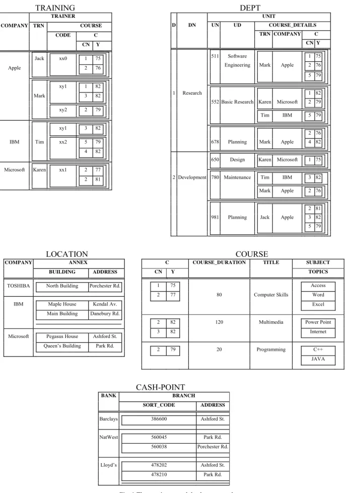
The running nested database example of the paper consists of five nested relations TRAINING, DEPT, LOCATION, CASH-POINT and COURSE (Fig. 1).
TRAINING
TRAINER COMPANY TRN COURSE CODE C CN Y Jack xx0 1 75 Apple 2 76 xy1 1 82 Mark 3 82 xy2 2 79 xy1 3 82 IBM Tim xx2 5 79 4 82 Microsoft Karen xx1 2 77 2 81DEPT
UNIT D DN UN UD COURSE_DETAILS TRN COMPANY C CN Y 511 Software 1 75Engineering Mark Apple 2 76
5 79
1 Research 1 82
552 Basic Research Karen Microsoft 2 79
Tim IBM 5 79
2 76
678 Planning Mark Apple 4 82 650 Design Karen Microsoft 1 75 2 Development 780 Maintenance Tim IBM 3 82
Mark Apple 2 76
2 81
981 Planning Jack Apple 3 82
5 79
LOCATION
COMPANY ANNEX
BUILDING ADDRESS
TOSHIBA North Building Porchester Rd. IBM Maple House Kendal Av.
Main Building Danebury Rd.
Microsoft Pegasus House Ashford St. Queen’s Building Park Rd.
COURSE
C COURSE_DURATION TITLE SUBJECT CN Y TOPICS
1 75 Access
2 77 80 Computer Skills Word
Excel
2 82 120 Multimedia Power Point
3 82 Internet 2 79 20 Programming C++ JAVA
CASH-POINT
BANKBRANCH SORT_CODE ADDRESS Barclays 386600 Ashford St. NatWest 560045 Park Rd. 560038 Porchester Rd. Lloyd’s 478202 Ashford St. 478210 Park Rd.
Relation TRAINING holds data about courses and trainers provided by IT companies. Semantically, the attributes of the TRAINING relation have the following meaning: COMPANY - company name, TRN - trainer name, CODE - course code, CN - course number Y - year in which the course was taken. A specific course can be identified uniquely by both course number (CN) and year (Y); a specific course consists of a number of different topics (see rel. COURSE) which can be given by different trainers belonging to different companies.
Relation DEPT holds data about departments of a company as well as trainers who have given courses to the staff of these departments. The semantics of the attributes of relation DEPT are: D - department number, DN - department name, UN – unit number, UD – unit description, TRN – trainer name, COMPANY – company name, CN - course number and Y - year in which the course was taken. Relation DEPT is a modified version of relation DEPT in [5].
Relation LOCATION contains data about branches of different companies. The attributes of relation LOCATION have the following semantics: COMPANY –company name, BUILDING – building name and ADDRESS – street name.
Relation CASH-POINT has data about cash-points that different banks own. The semantics of the attributes of relation CASH-POINT are: BANK – bank name, SORT_CODE – sort code of the branch and ADDRESS – street name.
Relation COURSE contains data about the different courses that took place. Semantically, the meaning of the attributes of relation COURSE is: CN - course number, Y - year in which the course was taken, COURSE_DURATION – course duration (number of hours), TITLE – course title and TOPICS – course topics.
IV. BASIC CONCEPTS AND TERMINOLOGY
In order to introduce the Nested Relational Model (NRM) in the next section it is necessary to present firstly the basic concepts and terminology that are going to be used. Some of the following definitions have been used before by the database community. However, a repetition of these definitions at the present point is necessary for completeness. Moreover, some terms and notation are introduced for the first time in the present paper in order to provide the essential formalisation of the presented model.
Definition 1(Atomic or flat attributes and relation-valued or nested attributes) Let U be the set of elementary values
(i.e., reals, integers etc.) and the value null. An attribute A is atomic or flat if DA ⊆ U, where DA is the domain of the
attribute A. If DA⊆ P(U) where P is the power set, then A is a
relation-valued or nested attribute.
Relation-valued attributes or nested attributes can be considered as subrelations of the relations to which they belong.
Definition 2 (Non-first normal form relations or nested relations) Non-first normal form relations or nested relations
are relations which contain relation-valued attributes or nested
attributes.
In this paper, relations with atomic attributes only will be called flat relations, whereas relations that contain relation-valued attributes or atomic attributes will be referred to as nested relations. In other words, flat relations are considered as special cases of nested relations.
Attr(R) is the set of attributes of relation r with scheme name R i.e., Attr(R) = {R1, R2, ..., Rn}, where n ≥ 1 and R1,
R2, ..., Rn are the attributes of R, either atomic or nested. Definition 3(Tree structure) Every nested relation r with
relation scheme R can be represented as a tree with root node R. All the nested attributes of the relation are the non-leaf nodes of the tree and all the atomic attributes form the leaf nodes of the tree.
The tree structure is a very useful representation of a nested relation since the scheme of a nested relation can become complex and so, the tree offers a clear graphical representation of the nested structure.
Example 1: The tree structure of the TRAINING relation (Fig. 1) is shown in Fig. 2.
Definition 4 (Nesting levels of a relation) The number of
nesting levels of a relation is equal to the maximum number of nodes to be passed through starting from the root to reach any atomic attribute in the tree representation. The root of the relation is by definition at nesting level 0.
Example 2: The nesting levels of relation TRAINING (Fig.
1) are 4.
Consequently, the nesting level of an attribute in a relation can be computed by counting the number of nodes which must be passed through from the root node to get to that attribute. For example, atomic attribute TRN of relation TRAINING is at nesting level 2.
Definition 5 (Common attributes between two relations)
Two (flat or nested) relations have an atomic attribute in common if they both contain an atomic attribute which has the same name and domain in both relations. Two nested relations have a nested attribute in common if they both contain a nested attribute which has the same name and the same scheme (the same atributes with the same names defined over
TRAINING
COMPANY TRAINER TRN COURSE
CODE C
CN Y
the same domains).
The above definition can be applied recursively for nested attributes containing one or more nested attributes.
Definition 6 (Path) Let LAn→Aj be the path of nested or
atomic attribute Aj belonging to nested attribute An, which is a
child of the root of relation R. Then, LAn→Aj is defined as
follows:
i) LAn→Aj = An, where Aj = An
ii) LAn→Aj = An(LAn+1→Aj), where An+1 is an attribute of An
either equal to or containing Aj.
Then, the set of all attributes (atomic and nested) of R can be defined as Attr(R) = {Ra1, Ra2, …, Rap, Rn1, …, Rni, …, Rnq} = {Ra1, Ra2, …, Rap, Rn1, …,
∪
m k=0 LRni → Rni k , …, Rnq} where: Ra1, Ra2, …, Rap are atomic attributes at nesting level
1 of relation R (p ≥ 0),
Rn1, …, Rni, …, Rnq are nested attributes at nesting
level 1 of relation R (1 ≤ i ≤ q), Rni for k = 0
Rni
k= Rni
k for k ≠ 0 (i.e., an attribute that has nested attribute Rni as its ancestor)
m is the number of descendants’ attributes of nested attribute Rni.
The path is used for the definition of an attribute in a nested relation, in contrast to flat relations, since the whole path of an attribute is needed in order to identify that specific attribute.
Example 3: The path of the atomic attribute CN of the
nested relation TRAINING (Fig. 1) with tree structure in Fig. 2 is LTRAINER→CN = TRAINER(LCOURSE→CN) =
TRAINER(COURSE(LC→CN)) =
TRAINER(COURSE(C(LCN→CN))) =
TRAINER(COURSE(C(CN))).
From the above example, it is apparent that the name of an attribute by itself is not enough in general to uniquely identify the attribute, since in nested relations an attribute is fully defined by reference to both its name and its position in the tree structure of the relation in which it belongs. In addition, there are cases in which two common attributes belong in the same relation but in different subrelations, as for example in the result relation of a join operation. Consequently, the only way for the two attributes to be distinguished from one another is by their paths. Therefore, the path of an attribute shows whether the attribute belongs to a nested attribute or not, as well as the nesting level of it. The path of an attribute identifies the attribute uniquely.
Definition 7 (Two nested relations having the same scheme) Two nested relations have the same scheme if they
contain only common attributes (atomic and/or nested) -see Definition 5.
An attribute or set of attributes whose values uniquely identify each entity in an entity set is called a key for that
entity set [21]. For the case of a nested database model, entity sets are nested relations and the definition of the key must be expanded in order to support nested attributes as well.
Informally, a nested relation can have either atomic or nested attributes or even a combination of atomic and nested attributes as a key. Semantically, a nested attribute is a key of a nested relation, when each set of values of the nested attribute that belongs to the same tuple, uniquely identifies that tuple. That implies that each of these set of values of the nested attribute distinguishes, as an entirety, solely the tuple in which it belongs.
Formally, the definition of a key of a nested relation is given below:
Definition 8 (Key of a nested relation) The key of a nested
relation r with relation scheme R, can be a set K consisting of atomic and/or nested attributes of R such that for any two tuples ti and tj in the relation the following constraint is valid
at all times: ti[K] ≠ tj[K], where i ≠ j and with the additional
property that removing any attribute from K leaves a set of attributes that is not a key of R.
Example 4: The key of relation COURSE (Fig. 1) is the
nested attribute C.
It is considered that an approach where nested attributes are allowed to be part of key attributes is an important benefit for a nested model. Nested models, where nested attributes are not allowed to be part of key attributes, have a significant limitation, since relations, as the one presented in Fig. 1, cannot be supported. Therefore, there are cases that are not covered by such an approach.
The PNF assumption presupposes that nested attributes cannot form part of a key in a nested relation, a significant restriction of a nested database model, as explained in section II.
Consequently, in the nested model defined in the present paper, the relaxing of the restriction that other nested models impose, to allow nested attributes as part of the key, is a considerable extension and thus, an important benefit that the NRM offers.
V. THE NESTED RELATIONAL ALGEBRA (NRA)
A new nested relational algebra is defined in this chapter, called the Nested Relational Algebra, NRA. Relations in NRA can be nested to any finite depth.
A. Operations in the NRA
Union, difference, intersection, projection, selection, unnest, nest, rename, Cartesian product, natural join and Θ– join operations are formally defined using recursive definitions for nested relations. The “base case” of each recursive operator has the same definition as the non-recursive one; i.e., the recursive definition can be reduced to the non-recursive one when relations do not contain any nested attributes. For each definition, an example is presented in order to make it more comprehensive. The recursive rename operation for nested relations is also formally defined for the first time.
For the recursive nested union, difference and intersection operations let r and q be two nested (in general) relations with relation schemes R and Q respectively. Let also, the two relations have the same relation scheme i.e., R = Q = {S(R), R1, R2, …, Rn} where S(R) is the set containing all the key
nested attributes and all the atomic attributes of R and Q (the same for the two relations) and {R1, R2, …, Rn} are the
non-key nested attributes of R and Q. Assume also that Attr(R) is the set of all attributes (atomic and nested) of the two relations, tr is a tuple in relation r, tq is a tuple in relation q and
t is a tuple in the result relation.
The Recursive Nested Union Operation (∪∪)
The union of the two relations r and q, r ∪∪ q, is defined as
follows:
Definition 9 (Recursive Nested Union)
i) Non-recursive union for flat relations (r ∪ q)
r ∪ q = { t| ((∃ tr∈ r) (t[Attr(R)] = tr[Attr(R)]))
∨ ((∃ tq∈ q) (t[Attr(R)] = tq[Attr(R)]))}
ii) Recursive union for nested relations (r ∪∪ q)
r ∪∪ q = { t| ((∃ t ∈ r) ∧ (∀ t q∈ q) (t[S(R)] ≠ tq[S(R)])) ∧ ((∃ t ∈ q) ∧ (∀ tr∈ r) (t[S(R)] ≠ tr[S(R)])) ∧ ((∃ tr∈ r) (∃ tq∈ q) ((t[S(R)] = tr[S(R)] = tq[S(R)]) ∧ (t[R1] = tr[R1] ∪∪ tq[R1]) ∧…∧ (t[Rn] = tr[Rn] ∪∪ tq[Rn])))}
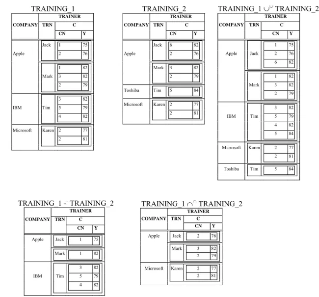
Example 5: Let relations TRAINING_1 and TRAINING_2
(Fig. 3) be two modified versions of relation TRAINING (Fig. 1) having the same scheme. In both relations, TRAINING_1 and TRAINING_2, S(TRAINING_1) = S(TRAINING_2) = COMPANY.
The union of the two relations, according to the above definition, is shown in Fig. 3.
The Recursive Nested Difference Operation (--)
TRAINING_1 ∪∪TRAINING_2 TRAINER COMPANY TRN C CN Y 1 75 Apple Jack 2 76 6 82 1 82 Mark 3 82 2 79 3 82 IBM Tim 5 79 4 82 5 84 Microsoft Karen 2 77 2 81 Toshiba Tim 5 84 TRAINING_2 TRAINER COMPANY TRN C CN Y Jack 6 82 Apple 2 76 Mark 3 82 2 79 Toshiba Tim 5 84 Microsoft Karen 2 77 2 81 TRAINING_1 -- TRAINING_2 TRAINER COMPANY TRN C CN Y Apple Jack 1 75 Mark 1 82 3 82 IBM Tim 5 79 4 82 TRAINING_1 ∩∩ TRAINING_2 TRAINER COMPANY TRN C CN Y Apple Jack 2 76 Mark 3 82 2 79 Microsoft Karen 2 77 2 81 TRAINING_1 TRAINER COMPANY TRN C CN Y Jack 1 75 Apple 2 76 1 82 Mark 3 82 2 79 3 82 IBM Tim 5 79 4 82 Microsoft Karen 2 77 2 81
The difference of the two relations r and q, r -- q, is defined
as follows:
Definition 10 (Recursive Nested Difference)
i) Non-recursive difference for flat relations (r - q) r - q = { t| (∃ tr∈ r) (∀ tq∈ q) ((t[Attr(R)] = tr[Attr(R)]) ∧ (t[Attr(R)] ≠ tq[Attr(R)]))}
ii) Recursive difference for nested relations (r –- q)
r -- q = { t| ((∃ t r∈ r) (∀ tq∈ q) ((t[S(R)] = tr[S(R)] - tq[S(R)]) ∧ (t[R1] = tr[R1]) ∧…∧ (t[Rn] = tr[Rn]))) ∨ ((∃ tr∈ r), (∃ tq∈ q) ((t[S(R)] = tr[S(R)] = tq[S(R)]) ∧ (t[R1] = tr[R1] -- tq[R1]) ∧…∧ (t[Rn] = tr[Rn] -- tq[Rn])))} Example 6: The difference of the two relations
TRAINING_1 and TRAINING_2 is shown in Fig. 3. The Recursive Nested Intersection Operation (∩∩)
The intersection of the two relations r and q, r ∩∩ q, is
defined as follows:
Definition 11 (Recursive Nested Intersection)
i) Non-recursive intersection for flat relations (r ∩ q) r ∩ q = { t| (∃ tr ∈ r) (∃ tq∈ q) (t[Attr(R)] = tr[Attr(R)] =
tq[Attr(R)])}
ii) Recursive intersection for nested relations (r ∩∩q)
r ∩∩q = { t| (∃ t
r ∈ r) (∃ tq ∈ q) ((t[S(R)] = tr[S(R)] ∩
tq[S(R)])
∧ (t[R1] = tr[R1] ∩∩ tq[R1]) ∧ ... ∧ (t[Rn] = tr[Rn] ∩∩
tq[Rn]))}
Example 7: The intersection of the two relations
TRAINING_1 and TRAINING_2 is shown in Fig. 3. The Recursive NestedProjection Operation (ππ)
Let r be a nested (in general) relation with relation scheme R. Let also, {Ra1, …, Rak} be the subset of atomic attributes at
the top level of R which are going to be projected and {Rn1,
…, Rnm} the subset of nested attributes of R which are going
to be projected either fully or partially on attributes belonging to these nested ones (k, m ≥ 0).
In order to define the projection operation, the term project list needs to be defined firstly. In general, a project list is a list of project paths. A project path of an attribute which is going to be projected is the path of that attribute (see Definition 6).
Definition 12 (Project list) Lπ is a project list of R if
i) Lπ is empty (the project list of an atomic attribute is
empty).
ii) Lπ is of the form (Rn1Ln1, …, RnmLnm), where Ln1, …, Lnm
are project lists of nested attributes Rn1, …, Rnm respectively.
Then, the projection operation in a nested relation r,
ππ(rL
π), where tr is a tuple in relation r and t is a tuple in the
result relation, is defined as follows:
Definition 13 (Recursive Nested Projection)
i) π(r) = r ii) ππ(r(R a1, …, Rak, Rn1Ln1, …, RnmLnm)) = { t| (∃ tr∈ r) ((t[Ra1] = tr[Ra1]) ∧ … ∧ (t[Rak] = tr[Rak]) ∧ (t[Rn1] = ππ(tr[Rn1]Ln1)) ∧ … ∧ (t[Rnm] = ππ(t r[Rnm]Lnm)))}
Example 8: Given relation TRAINING_1 (Fig. 3) consider
the following query: “Retrieve the course numbers for the courses that each company has run”. The result relation is
shown in Fig. 4.
The Recursive NestedSelection Operation (σσ)
Let r be a nested (in general) relation with relation scheme R and let Ra = {Ra1, …, Rak} and Rn = {Rn1, …, Rnm} be the
subsets of all atomic and nested attributes of R respectively that participate in the selection operation, where k and m are less than or equal to the number of atomic and nested attributes at the top level in the relation R, respectively. Let also, c be a set of conditions in R, which is of the form {ca, cn}
where ca={ca1, …, cak} is a set of conditions which must be
true for the atomic attributes Ra1, …, Rak of R respectively and
cn ={cn1, …, cnm} is a set of conditions that must hold for the
nested attributes Rn1, …, Rnm of R respectively. When both
sets of conditions are applied simultaneously then, the result is obtained by computing the intersection of the two results. In addition, the condition can be no matter complicated, as for example equality of nested attributes. If two multi-valued nested attributes are compared for equality, they are treated as sets so, since each nested attribute is, in fact, a relation, equal tuples are searched at the level of the nested relations.
In order to define the selection operation, the term select list needs to be defined firstly. In general, a select list is a list of select paths. A select path of an attribute that is going to participate in the selection, is the path of that attribute (see Definition 6). The select list is defined recursively.
Definition 14 (Select list) Lσ is a select list of R if
i) Lσ is empty (all the atomic attributes of relation r have
empty select lists).
ii) Lσ is of the form (Rn1Ln1, …, RnmLnm) where Ln1, …, Lnm
are select lists of nested attributes Rn1, …, Rnm respectively.
Then, a selection operation of the relation r, where tr is a
tuple in relation r and t is a tuple in the result relation, is
TRAINER COMPAN Y C CN 1 2 Apple 1 3 2 3 IBM 5 4 Microsoft 2 2
defined as follows:
Definition 15 (Recursive Nested Selection) σ(rca1, …, cak) = { t| (∃ tr∈ r) ((t[Attr(R) - {Ra1, …, Rak}] = tr[Attr(R) - {Ra1, …, Rak}]) ∧ ((t[Ra1] = tr[Ra1]) ∧ ca1 = true) ∧ … ∧ ((t[Rak] = tr[Rak]) ∧ cak = true))} σσ(r cn1, …, cnmLσ) = { t| (∃ tr∈ r) ((t[Attr(R) - {Rn1, …, Rnm}] = tr[Attr(R) - {Rn1, …, Rnm}]) ∧ (t[Rn1] = σσ(tr[Rn1]cn1Ln1) ≠∅) ∧ … ∧ (t[Rnm] = σσ(tr[Rnm]cnmLnm) ≠∅))}
In the general case, the selection operation can be defined as the intersection of the two previously defined cases as follows:
σσ(r
cLσ) = σσ(rca1, …, cak, cn1, …, cnmLσ) = σ(rca1, …, cak) ∩σσ(rcn1, …, cnmLσ)
Example 9: Given relation TRAINING_1 (Fig. 3) consider
the following query: “Find all the information of the TRAINING_1 relation of those courses that have been given by trainers Mark or Tim during the year 1982”. The result is shown in Fig. 5.
The Recursive Unnest Operation (μμ)
Let r be a nested (in general) relation with relation scheme R.
Definition 16 (Unnest list) Lμ is an unnest list of R if it is
of the form
Ri, where Ri is a nested attribute of R at the top level.
(RiLi) where Li is an unnest list of the nested attribute Ri.
Let Attr(R) be the set of all attributes of R and Ri a nested
attribute of R, at the top level of R. Let also, tr be a tuple in
relation r and t a tuple in the result relation. Then, the unnest operation, μμ(r
Lμ), is defined as follows (see also [13]): Definition 17 (Recursive Unnest)
i) μ(rRi) = { t| (∃ tr∈ r) ((t[Attr(R) - Ri] = tr[Attr(R) - Ri]) ∧
(t[Ri] є tr[Ri]))}
ii) μμ(r
RiLi) = { t| (∃ tr ∈ r) ((t[Attr(R) – Ri] = tr[Attr(R) –
Ri])
∧ (t[Ri] = μμ(tr[Ri]Li)))}
Example 10: The result of unnesting relation TRAINING
(Fig. 1) on the COURSE attribute, i.e.,
μμ(TRAINING
TRAINER(COURSE)), is shown in Fig. 6.
The Recursive Nest Operation (vv)
Let r be a nested (in general) relation with relation scheme R.
Definition 18 (Nest list) Lv is a nest list of R if it is of the
form
i) (R1, …, Rn) where R1, …, Rn are attributes of R, either
atomic or nested at the top level of R.
ii) (RiLi) where Li is a nest list of the nested attribute Ri.
Let Attr(R) be the set of all attributes of R and An = {R1,
…, Rn} the set of attributes of R that are going to be nested to
form a new nested attribute A.
Let also, tr be a tuple in relation r, t a tuple in the result
relation and s a tuple of the new nested attribute A. Then, the nest operation, vv(r
Lv→A), is defined as follows (see also [13]): Definition 19 (Recursive Nest)
TRAINER COMPAN Y TRN C CN Y Apple Mar k 1 8 2 3 8 2 IBM Tim 3 8 2 4 8 2
Fig. 5 σσ(TRAINING_1((TRAINER(TRN) = ‘Mark’ OR ‘Tim’) AND (TRAINER(C(Y)) = 82))) TRAINER COMPAN Y TRN CODE CN Y Jack xx0 1 7 5 2 7 6 Apple Mark xy1 1 8
2 3 8 2 Mark xy2 2 7 9 Tim xy1 3 8 2 IBM Tim xx2 5 7 9 4 8 2 Microsoft Karen xx1 2 7 7 2 8 1 Fig. 6 μμ(TRAINING TRAINER(COURSE))
i) v(rAn→A) = { t| (∃ tr ∈ r) ((t[Attr(R) - An] = tr[Attr(R) -
An])
∧ (t[A] = {s[An] | (s є r) (s[Attr(R) - An] = tr[Attr(R) -
An])}))}
ii) vv(r
(RiLi) →A) = { t| (∃ tr∈ r) ((t[Attr(R) – Ri] = tr[Attr(R) –
Ri])
∧ (t[Ri] = vv(tr[Ri]Li→A)))}
Example 11: In order to return to relation TRAINING (Fig.
1) from the relation μμ(TRAINING
TRAINER(COURSE)) of Fig. 6, a
nest operation needs to be performed, i.e., vv(μμ(TRAINING
TRAINER(COURSE))TRAINER(CODE,C)→
TRAINER(COURSE)).
The Recursive Nested Rename Operation (ρρ)
The rename operation takes a specified relation and returns another that is identical to the given one except that at least one of its attributes has a different name ([22]). The rename operation is useful before or after performing a number of operations, as for example for cases when there are duplicate names in the result relation after performing a join operation of two relations, or when the Cartesian product operation is performed between two relations having attributes with the same name. When a rename operation takes place only the heading of the relation changes, the body (instance) remains the same.
Let r be a nested (in general) relation with relation scheme R = {R1, R2, …, Ri, …, Rn, A, B,…, Z}, where R1, R2, …, Ri,
…, Rn are atomic attributes and A, B, …, Z are nested
attributes at the top level of relation R.
Then, the rename operation, ρρ, of relation r is defined as
follows:
Definition 20 (Recursive Nested Rename)
i) Rename of an atomic attribute Ri to Ri´ at the top level of
relation R
ρ[Ri← Ri´](R) = {R1, R2, …, Ri´, …, Rn, A, B, …, Z}
ii) Rename of a nested attribute A to A′ at the top level of relation R ρ[A ← A′](R) = {R1, R2, …, Ri, ..., Rn,
∪
m k=0 LA´→Ak, B, …, Z}where m is the number of attributes that are descendants of A and for m = 0, A′= A0 (atomic attribute at the top level of
R) and case (ii) reduces to case (i).
iii) Rename of an atomic or nested attribute Ai to Ai′ at a
lower level of relation R ρρ[A
i ← Ai′](R) = {R1, R2, …, Ri, …, Rn, A, A1, …,
∪
mk=0
LA→Ai′k, B, …, Z}, where A1 is a child attribute of nested
attribute A, Ai is an attribute at a lower level of relation R
belonging to nested attribute A and m is the number of descendants that Ai has (m = 0, when atomic, in which case
Ai′0 = Ai′).
When more than one attribute has to be renamed the definition is recursive, as follows:
ρρ[R a1←R′a1, …, Rak←R′ak, Rn1←R′n1, …, Rnm←R′nm, Rl1←R′l1, …, Rlp←R′lp](R) = (ρρ[R lp←R′lp](…(ρρ[Rl1←R′l1](ρ[Rnm←R′nm](…(ρ[Rn1←R′ n1](ρ[Rak←R′ak](…(ρ[Ra1←R′a1](R))))))))))
where Ra1, …, Rak are atomic attributes at the top level of
relation R, Rn1, …, Rnm are nested attributes at the top level of
relation R and Rl1, …, Rlp are either atomic or nested attributes
at lower levels (different, in general) of relation R and k, m, p
≥ 0. The names of the attributes having primes denote the new names that these attributes are going to be renamed.
Example 12: Consider the relation DEPT (Fig. 1) and let
attribute UD be renamed as UD′ and attribute C as C′. Then, the rename operation is defined as follows:
ρρ[UD ← UD′, C ← C′](DEPT) = ρρ[C ← C′](ρρ[UD ←
UD′](DEPT)) =
ρρ[C ← C′]({D, DN, UNIT, UNIT(UN), UNIT(UD′),
UNIT(COURSE_DETAILS), UNIT(COURSE_DETAILS(TRN)), UNIT(COURSE_DETAILS(COMPANY)), UNIT(COURSE_DETAILS(C)), UNIT(COURSE_DETAILS(C(CN))), UNIT(COURSE_DETAILS(C(Y)))}) =
{D, DN, UNIT, UNIT(UN), UNIT(UD′),
UNIT(COURSE_DETAILS), UNIT(COURSE_DETAILS(TRN)), UNIT(COURSE_DETAILS(COMPANY)), UNIT(COURSE_DETAILS(C′)), UNIT(COURSE_DETAILS(C′(CN))), UNIT(COURSE_DETAILS(C′(Y)))}
The Recursive NestedCartesian Product Operation (××) Let R be a relation scheme of relation r.
Definition 21 (Join path) L is a join path of R if either:
(i) L is empty or
(ii) L = RiLi where Ri is a nested attribute of R and Li is a
join path of Ri. ([3])
The join path can be represented as a branch of the tree structure of some nested relation R starting from a child of the root of the tree and going down to some node of the tree that represents either an atomic or nested attribute. In other words, the join path consists of all the nodes that are passed in order to reach a specific attribute.
Example 13: In relation DEPT (Fig. 1) an example of a
join path is UNIT(COURSE_DETAILS(TRN)).
Let r and q be two nested (in general) relations with relation schemes R and Q respectively and let Attr(R) be all the attributes (atomic and nested) of R, Attr(Q) all the attributes (atomic and nested) of Q and L a join path of R. Let, also, Ri
be a nested attribute of R, Li a join path of Ri, tr a tuple in
relation r, tq a tuple in relation q and t a tuple in the result
relation. The Cartesian product operation can be applied either at the top level of both relations or between a lower nesting level of a relation and the top level of another relation. The first case is exactly the same as the standard Cartesian product for flat relations.
So, the Cartesian product of two relations r and q is defined as follows [13]:
Definition 22 (Recursive Nested Cartesian Product) × (r, q) = { t ≡ (t[Attr(R)], t[Attr(Q)])| (∃ tr ∈ r) (∃ tq ∈ q) ((t[Attr(R)] = tr[Attr(R)]) ∧ (t[Attr(Q)] = tq[Attr(Q)]))} ×× (rL, q) = ×× (r(R iLi), q) ≡×× (q, r(RiLi)) = { t| (∃ tr∈ r) ((t[Attr(R) –{Ri}] = tr[Attr(R) – {Ri}]) ∧ (t[Ri] = ×× (t r[Ri]Li, q)))}
The commutative property is satisfied, as is the case in the CRM. Thus, it is always valid that
×× (rL, q) ≡×× (q, rL)
Example 14: The Cartesian product operation is performed
between the COURSE attribute of relation TRAINING and the CASH-POINT relation (Fig. 1). Due to the large number of tuples in the result relation, only a part of it is displayed in Fig. 7.
The Cartesian product operation is not often a semantically meaningful operation, as can be seen from the above example. However, it helps in defining the join operation, since the join is a special case of a Cartesian product operation and for this reason it is included here.
The Recursive Nested Natural Join operation ( ) The natural join operation is formally defined in [23]. The main definition is given here for completeness reasons.
Definition 23 (Recursive Nested Natural Join)
Let r and q be two nested relations with relations schemes R and Q respectively and let A ={A0, A1, …, Aj} be the set of all
common attributes that the two relations have, where A0, A1,
…, Aj are atomic or nested attributes either at the top or lower
levels in the two relations.
Then, the natural join of relations r and q, (r, q), is defined as follows:
(r, q) = (sjLsjAj, s′jLs′jAj)(…( (s1Ls1A1,
s′1Ls′1A1)( (rLrA0, qLqA0)))) where (rLrA0, qLqA0) =
x1, (s1Ls1A1, s′1Ls′1A1) = x2, …, (sjLsjAj, s′jLs′jAj) =
xj+1 and (s1, s′1),…, (sj, s′j) pairs, are subrelations of x1, …, xj
respectively with their root node being the first different nodes along the paths to the common attributes A1, …, Aj
respectively.
The Recursive NestedΘ-Join Operation ( Θ )
The Θ-join operation is a special case of the join operation where the two relations are joined on the basis of some comparison operator other than equality.
It can be expressed by applying a selection operation to the result of the Cartesian product operation of two relations. The Cartesian product is applied at the top levels of the two nested relations and then, a recursive nested selection operation follows which compares two attributes in the resulting relation. The two attributes need not be at the same nesting
(TRN (CODE C BANK BRANCH)) COMPAN
Y
TRN (CODE C BANK BRANCH)
CODE BANK BRANCH
CN Y SORT_COD E ADDRESS xx0 1 7 5 Barclay s 386600 Ashford St. 2 7 6 Jack xx0 1 7 5 NatWes t 560045 Park Rd. 2 7 6 560038 Porchester Rd. xx0 1 7 5 Lloyd’s 478202 Ashford St. 2 7 6 478210 Park Rd. xy1 1 8 2 Barclay s 386600 Ashford St. Apple 3 8 2 xy1 1 8 2 NatWes t 560045 Park Rd. 3 8 2 560038 Porchester Rd. xy1 1 8 2 Lloyd’s 478202 Ashford St. 3 8 2 478210 Park Rd. Mar k xy2 2 7 9 Barclay s 386600 Ashford St. xy2 2 7 9 NatWes t 560045 Park Rd. 560038 Porchester Rd. xy2 2 7 9 Lloyd’s 478202 Ashford St. 478210 Park Rd. . . . . . . . . . . . . . . . . . . . . . . . .
level in the resulting relation.
Let r and q be two nested (in general) relations with relation schemes R and Q respectively. Let also, X and Y be two atomic attributes belonging to relations R and Q respectively and Θ the condition that they must satisfy. Assume, without loss of generality, that Y belongs to a deeper nesting level than X and LσY′→Y is the select path of Y starting at node Y′
which is at the same nesting level as X (when X and Y are at the same nesting level the select path is empty). So, the recursive nested Θ–join operation of the two relations r and q is defined as follows:
Definition 24(Recursive Nested Θ-Join)
r Θ q = σσ((r × q)X Θ Y Lσ Y′→Y)
B. Functions
Aggregate functions for nested relations have not been discussed in any other model presented in section II, but in [18]. Aggregate functions are redefined below.
Let f be a nested aggregate function (f є {N-MAX, N-MIN, SUM, AVG, COUNT}, where MAX, MIN, N-SUM, N-AVG and N-COUNT are the nested versions for the corresponding aggregate functions MAX, MIN, SUM, AVG and COUNT for flat relations), f′ an aggregate function for flat relations (f′ є {MAX, MIN, SUM, AVG, COUNT}), r a nested relation, X an atomic or nested attribute at a lower nesting level of r, Par the parent attribute of atomic attribute Y of r (Y is at the same or higher nesting level than X and it is the attribute over which attribute X is summarised) and X/Y denotes that attribute X is summarised over attribute Y. Then, f[X/Y](r) is defined as follows:
Definition 25 (Nested Aggregate Function)
f[X/Y](r) = f′({ti[X] | tiє t, t є Par(Y) ∧ ti[X] ≠ null})
Note: Attribute X can be a nested attribute only when the nested aggregate function f is N-COUNT. For all other cases, X attribute must be an atomic attribute.
For an example see Query 6 in section VI. VI. MANAGEMENT OF NESTED DATA
The nested algebra presented in section V, is a well-defined and formalised nested algebra where data restructuring operations are avoided. In this section, examples are provided to show the ease of use of the NRA. Relations have no restrictions on the number of nesting levels they can contain. The nested model presented, provides a better way of representing and querying complex data as demonstrated by the queries that follow since they are compact and do not require nest, unnest or any other restructuring operations for the manipulation of nested data.
A number of examples are presented that contain only operations on nested data, demonstrating how this model works and functions. Queries refer to the nested database example described in section III (Fig. 1). For some queries, comparisons are made with other proposed models.
Query 1: What are the descriptions of the units that belong
to department 1 and who are the trainers who have given
courses to staff members of these units? Display also the value for the department.
ππ((σσ(DEPT
D = 1)) D, UD, TRN)
A projection operation on a selected part of the DEPT relation is needed to answer the above query. Three attributes of the relation are projected which can be found at different nesting levels; attribute D at nesting level 1, attribute UD at nesting level 2 and attribute TRN at nesting level 3. However, the projection operation takes place as normal, without changing the structure of the relation using unnest and nest operations and thus, the nesting arrangement of the relation is maintained in the resulting relation as well. Therefore, in the resulting relation, D, UD and TRN are still at nesting levels 1, 2 and 3 respectively, as in the input relation DEPT.
Query 2: Find the tuples with course numbers equal to the
number of the department for the whole tuple.
σσ(DEPT
D = CN)
The above query shows the advantage of the selection operation proposed in section V that allows arbitrary expressions to be specified in the select condition, as for example equality of values of attributes that are not at the same nesting level in the relation, without unnesting and nesting the relation. The query is expressed algebraically in exactly the same way as if the two compared attributes were at the top level of the original relation.
Query 3: Find the names of the banks and the companies
that are situated at the same road.
νν((μμ(ππ((LOCATION CASH-POINT)
COMPANY,BANK,ADDRESS))(ADDRESS))(COMPANY,BANK)→( COMPANY BANK))
In this example, and in similar cases, nest and unnest operations are necessary since they can restructure the relations and as a result, present the same data in a different format that is required by the given query.
However, extra nest and unnest operations are avoided in the above query since the natural join and projection operations are defined recursively in the NRA.
In Abiteboul and Bidoit’s model [1] this query cannot be performed since the two relations that participate in the natural join operation do not have any common attributes at the top level.
Query 4: Find the names of the trainers that have given the
“Computer Skills” training course.
ππ((σσ(TRAINING COURSE)
TITLE= “Computer Skills”)
TRN)
One can easily see the advantage of joining subrelations which are at different nesting levels (in this example, the subrelation C at nesting level 3 in relation TRAINING and at nesting level 1 in relation COURSE), without the need to unnest and nest the data and without any other restructuring operations assumed by other proposed models (e.g., [1], [13]). The above example shows that NRA provides a simple way of answering queries, since even just the algebraic solution of the query can be translated naturally to the above well-phrased query; moreover, the query does not distinguish between
nested and flat relations, as the query would be expressed in the same way if the two relations, TRAINING and COURSE, were flat relations. This is explained by the recursive nature of the NRA operations.
In contrast, in Levene’s model [14] the natural join can be applied only if relation COURSE is extended with two empty nodes at levels 1 and 2 so that the common attribute C to appear at the same nesting level 3 in both relations. Then, the two relations are joinable, according to Levene’s definition and therefore, can be joined.
Query 5: Find the names of the banks which are located on
the same road as the companies for which Tim or Karen have worked for, together with the names of these companies.
ππ((((σσ(TRAINING
(TRN= “Tim” OR TRN = “Karen”)))
LOCATION) CASH-POINT) COMPANY, BANK) This query requires two natural join operations. However, since the natural join defined in [23] can be performed between any possible relations sharing common attributes, it does not involve any preliminary checks to determine if the two operand relations are qualified for the natural join. In other models, for example in [1], [13], it is not certain if the natural join operation can be performed between a nested relation and the output of the natural join of two nested relations, since, as explained in section II of this paper, for each of these models the natural join operation is subject to some restrictions. On the other hand, in NRA any possible combination of relations, sharing at least one common attribute, can be joined.
This query also demonstrates how complex queries can be answered easily in the query language proposed in this paper.
Query 6: What is the title of the course that has the
maximum number of different topics? Display also the number of different topics that this course has.
ππ(COURSE(TITLE,
N-COUNT[TOPICS/TITLE]←MTOPICS)) ππ(ππ(COURSE(TITLE,
N-COUNT[TOPICS/TITLE]←MTOPICS1)) (MAX(MTOPICS1)) ←MTOPICS)
Aggregate functions for nested attributes have been defined in subsection B of section V.
The above query is expressed in the NRA using the following steps:
1. In the original relation COURSE, the number of different topics per title is computed, it is named MTOPICS1 and projected on TITLE and MTOPICS1 attributes.
2. From the result of step 1, MAX (MTOPICS1) is computed, named MTOPICS and projected.
3. In the original relation COURSE, the number of different topics per title is computed, it is named MTOPICS and projected on TITLE and MTOPICS.
4. The results of steps 2 and step 3 are joined together. It is noteworthy that if the relation COURSE was a flat relation then, the SUMMARIZE operation would be used to produce the same result in combination with the traditional
aggregate functions COUNT and MAX.
It must be said that this query or any other query containing aggregate functions on nested attributes cannot be expressed in any other relational model discussed in section II apart from [18] with the use of an additional operator, the subrelation constructor, as follows:
π[TITLE, MAX[SUBJECT′]] (∮(C,
COURSE_DURATION, TITLE, SUBJECT, SUBJECT′); SUBJECT′ := COUNT[TOPICS](SUBJECT)∮ (COURSE)) where ∮ is the subrelation constructor.
Query 7: Find all trainers who have given more courses
than Karen has.
ππ((σσ
(ππ((νν(μμ(π
tπ(TRAINING(TRN,COURSE))COURSE) (CODE, C)→COURSE))(TRN,N-COUNT[CN/TRN]←MCN)) ×× ππ((σσ(TRAINING
TRN= “Karen”))
(N-COUNT[CN/TRN]←MCN1))) MCN > MCN1) TRN)
Two copies of the TRAINING relation are needed for this query in order to perform the Cartesian product operation between them. However, to make the query simpler, a projection operation is applied to the first copy of the relation and an aggregate function is also used to count the number of nested tuples which corresponds to the number of different courses that each trainer (TRN) has given. Moreover, an unnest and then a nest operation are also used to a projected part of the original relation to convert the relation to the right one, before the computation of the aggregate function. With the second copy of the relation, a projection is performed on a selection of the relation. The same aggregate function is also used here, applied to the same attribute as before. The Cartesian product is performed afterwards between a binary relation and a unary one containing only one tuple.
Once again, the above query can demonstrate the expressive power of the proposed nested model and the facility in stating complex queries. This query, as the previous one, cannot be expressed in any other nested relational model presented in section II apart from [18], yet with the problem discussed above.
VII. THE NESTED RELATIONAL MODEL (NRA)
The components of the NRM are described below. A. Data types-Domains
Domains are data types of arbitrary internal complexity ([22]). Therefore, such domains can consist of relation-type values. Attributes defined on that domains are relation-valued attributes, that is, they contain values that are relations. The domain of a nested attribute is defined recursively below.
Assume that Rn1, Rn2, …, Rnk are, in general, all the atomic
and nested attributes that belong to nested attribute Rn and P is
the powerset of a set S.
Definition 26 (Nested attribute domain) The domain of a
nested attribute Rn, DOM(Rn), is defined recursively as
i) DOM(Rn) ⊆ D, where D is the underlying database
ii) DOM(Rn1) × DOM(Rn2) × … × DOM(Rnk), for k ≥ 1,
where Rn1, Rn2, …, Rnk are atomic attributes of Rn.
iii) P(DOM(Rn1)) × P(DOM(Rn2)) × … × P(DOM(Rnk)), for
k ≥ 1, where Rn1, Rn2, …, Rnk are nested attributes of Rn, in
general.
B. Databases
In the NRM, databases are sets of nested relations. Nested relations do not satisfy the 1NF assumption. A database example in the NRM is shown in Fig. 1.
C. Structures
Definition 27 (Nested Relation Scheme) The scheme of a
relation R in the NRM is defined recursively asRS = R(R1S1,
R2S2, ..., RnSn), where n ≥ 1, R1, R2, ..., Rn are the attribute
names of R, either atomic or nested and
∅ (empty set) if Ri is an atomic attribute
Si =
(Ri1S i1, Ri2S i2, ..., RikSik) if Ri is a nested attribute
and k ≥ 1 where 1 ≤ i ≤ n.
Example 15: The scheme of relation TRAINING (Fig. 1) is
TRAINING (COMPANY TRAINER (TRN COURSE (CODE C (CN Y)))).
D. Relational Operators
The set of conventional relational comparison operators of the CRM, {=, ≠, <, ≤, >, ≥}, is also supported in the NRM.
E. Operations
The union, difference, intersection, projection, selection, rename, Cartesian product, natural join and Θ-join recursive operations of the NRM have been defined formally in section V. Two additional operations, nest and unnest, have also been defined in the NRM.
F. Functions
The set of functions in the CRM is also supported in the NRM.
VIII. MAPPING THE CRM TO THE NRM
NRM is reduced to the CRM when restricted to support only flat relations, in a way similar to the approach of Paredaens and Van Gucht [24]. In this section, the components of the CRM are going to be mapped to the NRM that have been described in section VII, in order to prove that the NRM is a proper superset of the CRM.
A. Data types - Domains
Proposition 1: The set of domains in the CRM is a proper
subset of the set of domains in the NRM.
Proof: The nested attribute domain is defined recursively
(Definition 26). Therefore, for the special cases i) where k=0 i.e., the attribute is atomic or ii) where k ≥ 1 i.e., the attribute is nested consisting of atomic attributes only (which can be considered as a flat relation), the nested attribute domain definition of the NRM is reduced to the atomic attribute
domain definition of the CRM.
Consequently, since the set of domains in the NRM can be reduced, for specific special cases, to the set of domains in the CRM, the former is a proper superset of the set of domains in the CRM.
B. Databases
Proposition 2: The set of databases in the CRM is a proper
subset of the set of databases in the NRM.
Proof: Databases in the NRM have been introduced in
order to relax the 1NF assumption that is satisfied in the CRM. Thus, the 1NF assumption of flat relations is a special case of the general N1NF assumption which characterises relations in the NRM. By definition, a flat relation is also a relation of the nested model. Therefore, the set of databases in the NRM is a proper superset of the set of databases in the CRM.
C. Structures
Proposition 3: The set of structures in the CRM is a proper
subset of the set of structures in the NRM.
Proof: The definition of the scheme in the NRM is given
recursively (Definition 27). For the special case, where Si, for
all i, is equal to the empty set, the definition is reduced to that of the CRM, since all attributes of the relation are atomic.
D. Relational Operators
Proposition 4: The set of relational comparison operators
in the CRM is isomorphic to the set of relational operators in the NRM (i.e., for every comparison operator in the CRM there is a corresponding comparison operator in the NRM).
Proof: The proof is omitted for obvious reasons.
E. Operations
In the following, it is shown by a number of propositions that each operation in the NRM is an extended operation of the relevant operation in the CRM. Before this is done, some preliminary discussion is necessary, regarding the effect of relational operations to the key of relations.
Let Unary be a unary operation and let R1 = Unary(R0).
Then, the first obvious remark is that this operation does not have any effect on the key of R0 i.e., the key of R0 remains the
same. The second one is that the key of R0 is not inherited to
R1. These observations apply to any data model, and to the
CRM as well. As an example of the second remark, consider a flat relation R0 and assume that K is its primary key. Then, the
CRM select operation R1=σF(R0), also yields a flat relation,
R1. Since R1 is a subset of R0, it follows that it does not
contain two distinct tuples with identical values for K. However, it is not implied by this fact that K is also the key of R1, it is only the user who may specify what the key of R1 is.
As another example, let the scheme of R0 be R0(K, A, B),
where K is its key. If R1=πA,B(R0), it is known that R1 does not
contain duplicate tuples and, definitely, it is again the user who may specify its key.
Hence, the conclusion is that a unary CRM operation does not affect the key (if defined) of the input relation and it does
not propagate it to the result relation. This same conclusion can also be drawn for binary operations of the CRM. Subsequently, the same conclusion can be drawn for any operation in any data model, therefore for all the operations of the NRM as well.
Proposition 5: The union operation in the NRM is an
extended version of the union operation in the CRM.
Proof: The union operation in the NRM is defined
recursively (Definition 9). From the recursive definition, it is deduced that for the special case where the relations are in 1NF format, the definition is reduced to the non-recursive union definition for flat relations (case i), since the relations do not contain any nested attributes. This definition then, is the definition of the union operation in the CRM.
Proposition 6: The difference operation in the NRM is an
extended version of the difference operation in the CRM.
Proof: The proof is similar to that of Proposition 5.
Proposition 7: The intersection operation in the NRM is an
extended version of the intersection operation in the CRM.
Proof: The proof is similar to that of Proposition 5.
Proposition 8: The projection operation in the NRM is an
extended version of the projection operation in the CRM.
Proof: From Definition 13 (case ii): ππ(r(R a1, …, Rak, Rn1Ln1, …, RnmLnm)) = { t| (∃ tr∈ r) ((t[Ra1] = tr[Ra1]) ∧ … ∧ (t[Rak] = tr[Rak]) ∧ (t[Rn1] = ππ(tr[Rn1]Ln1)) ∧ … ∧ (t[Rnm] = ππ(t r[Rnm]Lnm)))}.
For the special case where relation r is flat, since all attributes of relation r are atomic, RniLni = ∅, for all i (1 ≤ i ≤
m), and the definition of the projection operation is reduced to:
ππ(r(R
a1, …, Rak, Rn1Ln1, …, RnmLnm)) = ππ(r(Ra1, …, Rak)) =
{ t| (∃ tr ∈ r) ((t[Ra1] = tr[Ra1]) ∧ … ∧ (t[Rak] =
tr[Rak]))},
which is the definition of the projection operation in the CRM. So, the projection operation in the NRM is an extended version of the projection operation in the CRM.
Proposition 9: The selection operation in the NRM is an
extended version of the selection operation in the CRM.
Proof: The proof is similar to that of Proposition 8. For the
special case where relation r is flat, since all attributes of relation r are atomic, L is empty and Definition 15 is reduced to σσ(r
cLσ) = σ(rc) = σ(rca1, …, cak) which is the traditional
selection operation for flat relations in the CRM.
Proposition 10: The rename operation in the NRM is an
extended version of the rename operation in the CRM.
Proof: From Definition 20-case (ii),therename of a nested
attribute at the top level of a relation is:
ρ[A ← A′](R) = {R1, R2, …, Ri, …, Rn,
∪
m
k=0
LA′→Ak, B, …,
Z}.
This definition is reduced to:
ρ[A ← A′](R) = {R1, R2, …, Ri, …, Rn, A′, B, …, Z}, for
the special case where the attribute to be renamed, A, is an
atomic attribute at the top level of relation R, since
∪
mk=0 LA′→Ak
= A′ (m=0 i.e., there are not any descendants of A). This is equivalent to the rename operation in the CRM.
Proposition 11: The Cartesian product operation in the
NRM is an extended version of the Cartesian product operation in the CRM.
Proof: Case (i) or case (ii) for L=Ø of Definition 22 is the
traditional Cartesian product operation for flat relations in the CRM.
Proposition 12: The natural join operation in the NRM is
an extended version of the natural join operation in the CRM.
Proof: The natural join which operates for cases where the
common atomic or nested attributes belong to different subrelations and at different nesting levels in the two relations), (rL, qM), is defined in [23].
The natural join can be reduced to the conventional natural join for flat relations if the special case is assumed, where the common attributes are atomic attributes at the top level of the two relations. Formally, the definition for L and M empty, is reduced to:
(rL, qM) = (r, q) = { t| (∃ tr∈ r) (∃ tq∈ q)
((t[Attr(Ri)] = tr[Attr(Ri)])
∧ (t[Attr(Qi)] = tq[Attr(Qi)])
∧ (t[Ri1] = tr[Ri1] = tq[Qi1]))}
which is the traditional definition of the natural join operation in the CRM.
F. Functions
Proposition 13: The set of functions in the CRM is
isomorphic to the set of functions in the NRM.
Proof: The proof is omitted for obvious reasons.
G. Mapping Synopsis
Proposition 14: The NRM is a superset of the CRM. Proof: This is a result of Propositions 1-13 since, as it has
been explained in subsection B of section VIII, in order to prove that a database model is a superset of another database model, it is necessary and sufficient to prove that every property of the latter (data types, databases, structures, operators, operations and functions) is also a property of the former.
IX. CONCLUSION
In this paper, an algebra (NRA) and a database model (NRM) have been defined for nested relations of arbitrary nesting levels. All the operators have been recursively defined. As a result, there is no need to flatten the nested relations when a series of operations are executed and so the data redundancy and duplication caused by unnesting relations is avoided. Furthermore, the representation of the data is claimed to be in a “natural form”. Thus, it is easier for users to understand when working with the data, since even complex objects can be modelled in one relation. A number of example queries have been expressed in the NRA to demonstrate its
functionality. In addition, the model has been proved to be consistent with the CRM.
In appendix I, a formal syntax of the NRA is given. In appendix II, a sample code of the prototype implementation can be found as well as a number of examples, presented in this paper, coded in Miranda, which demonstrate the functionality and validity of the model. It should be stated that the prototype serves satisfactory as a proof of concept. Specifically, the nested rename, projection, selection and Cartesian product operations have been fully implemented. The nested join operation has been partially implemented. Particularly, only one nested column is allowed at each nesting level and the join operator allows joining on only one pair of columns; reasonable assumptions within the framework of a prototype.
Future work includes the study of optimisation techniques for the efficient evaluation of complex queries. The definition of an extension of SQL to support the nested features of NRM is also, another research direction. The incorporation of spatial data to NRM is an additional challenge. The NRM can also be used as a basis to build an algebra for supporting nesting structures in XML (similarly to the FLWR expressions of XQUERY).
APPENDIX I
Formal syntax of the NRA expression
:: = one-relation-expression| two-relation-expression one-relation-expression
:: = nested-renaming | nested-selection | nested-projection two-relation-expression
:: = nested-projection binary-operation expression nested-renaming
:: = ρtρ [attribute-commalist1] (term)
attribute-commalist1
:: = fattribute ← fattribute | fattribute ← fattribute, attribute-commalist1 fattribute :: = attribute1 | function2(attribute1) attribute1 :: = attribute | nested-aggregate-attribute attribute :: = basic-attribute | nested-attribute basic-attribute :: = atomic-attribute nested-aggregate-attribute :: = function1[attribute/basic-attribute] function1
:: = N-MAX | N-MIN | N-SUM | N-COUNT | N-AVG function2
:: = MAX | MIN | AVG | COUNT | SUM term
:: = relation | (expression) nested-projection
:: = πtπ (term (attribute-commalist2)) | term
attribute-commalist2
:: = fattribute | fattribute, attribute-commalist2 binary-operation :: = ∪∪ | ∩∩ | −− | ×× | | Θ nested-selection :: = σσ(term comparison) comparison
:: = attribute-term | attribute-term logical-operator comparison
logical-operator
:: = AND | OR | AND NOT | OR NOT attribute-term
:: = FAA θ FAA FAA
:: = constant | atomic-attribute | attribute-term | nested-aggregate-attribute
θ
:: = < | > | = | <= | >= | ≠
APPENDIX II
A sample of the prototype implementation
A small part of the code, that has been developed in Miranda, is listed in this section which contains basic functions for selection, projection and Cartesian product operators.
|| isColumnTag: Simple method to identify a column using its tag.
isColumnTag :: string -> columnType -> bool
|| resolvePath: Creates full path name for columns in a table.
resolvePath:: relationalTable -> relationalTable
|| resolvePath2: Creates full path names for a list of entries given a string and a depth.
resolvePath2 :: string -> num -> [tableEntry] -> [tableEntry]
|| resolvePath3: Creates full path names for a list of columns given a string and a depth.
resolvePath3 :: string -> num -> tableEntry -> tableEntry
|| resolvePath4: Creates full path names for a column given a string and a depth.
resolvePath4 :: string -> num -> columnType -> columnType
|| rpar: Generates a given number of closing parenthesis.
rpar :: num -> string
|| selectCol: Used to select a column recursively based on its tag.
selectCol :: string -> columnType -> tableEntry