05 August 2020
Repository ISTITUZIONALE
User Interaction with Online Advertisements: Temporal Modeling and Optimization of Ads Placement / VASSIO, LUCA; Garetto, Michele; CHIASSERINI, Carla Fabiana; LEONARDI, Emilio. - In: ACM TRANSACTIONS ON MODELING AND PERFORMANCE EVALUATION OF COMPUTING SYSTEMS. - ISSN 2376-3639. - STAMPA. - 5:2(2020), pp. 1-26. Original
User Interaction with Online Advertisements: Temporal Modeling and Optimization of Ads Placement
acm_draft Publisher: Published DOI:10.1145/3377144 Terms of use: openAccess Publisher copyright
© {Owner/Author | ACM} {Year}. This is the author's version of the work. It is posted here for your personal use. Not for redistribution. The definitive Version of Record was published in {Source Publication}, http://dx.doi.org/10.1145/{number}
(Article begins on next page)
This article is made available under terms and conditions as specified in the corresponding bibliographic description in the repository
Availability:
This version is available at: 11583/2774773 since: 2020-03-09T12:43:42Z
User Interaction with Online Advertisements:
Temporal Modeling and Optimization of Ads Placement
LUCA VASSIO,
Politecnico di Torino, ItalyMICHELE GARETTO,
Università di Torino, ItalyCARLA CHIASSERINI,
Politecnico di Torino, ItalyEMILIO LEONARDI,
Politecnico di Torino, ItalyWe consider an online advertisement system and focus on the impact of user interaction and response to targeted advertising campaigns. We analytically model the system dynamics accounting for the user behavior and devise strategies to maximize a relevant metric called click-through-intensity (CTI), defined as the number of clicks per time unit. With respect to the traditional click-through-rate (CTR) metric, CTI better captures the success of advertisements for services that the users may access several times, making multiple purchases or subscriptions. Examples include advertising of on-line games or airplane tickets. The model we develop is validated through traces of real advertising systems and allows us to optimize CTI under different scenarios depending on the nature of ad delivery and of the information available at the system. Experimental results show that our approach can increase the revenue of an ad campaign, even when user’s behavior can only be estimated.
CCS Concepts: •Information systems→Social advertising;Social recommendation; Personalization; Display advertising;Social advertising;Social recommendation;Personalization;Social recommendation;
Social recommendation;Personalization;
Additional Key Words and Phrases: Online advertisements, Recommendation systems, Ads placement, CTR, User behaviour
ACM Reference Format:
Luca Vassio, Michele Garetto, Carla Chiasserini, and Emilio Leonardi. 2019. User Interaction with Online Advertisements: Temporal Modeling and Optimization of Ads Placement.ACM Trans. Model. Perform. Eval.
Comput. Syst.1, 1, Article 1 ( January 2019), 26 pages. https://doi.org/10.1145/3377144 1 INTRODUCTION
Online advertising is a market estimated in 2018 at more than 100 billion dollars, in the USA alone [3]. This success has largely arisen with the usage of automatic processes that enable highly targeted advertising. In this paper, we consider an online system for targeted advertising, as illustrated in Fig. 1. On one side, a Publisher provides an Ad Server with a stream of available slots, i.e., portions of the user’s navigation experience where ads can be inserted. On the other side, an Advertiser provides a stream of ads that can potentially fill in those slots. The Advertiser will manage the slots according to its advertisement campaign. A subset of the available slots is matched with ads
Authors’ addresses: Luca Vassio, Politecnico di Torino, Italy, luca.vassio@polito.it; Michele Garetto, Università di Torino, Italy, michele.garetto@unito.it; Carla Chiasserini, Politecnico di Torino, Italy, carla.chiasserini@polito.it; Emilio Leonardi, Politecnico di Torino, Italy, emilio.leonardi@polito.it.
Permission to make digital or hard copies of all or part of this work for personal or classroom use is granted without fee provided that copies are not made or distributed for profit or commercial advantage and that copies bear this notice and the full citation on the first page. Copyrights for components of this work owned by others than the author(s) must be honored. Abstracting with credit is permitted. To copy otherwise, or republish, to post on servers or to redistribute to lists, requires prior specific permission and /or a fee. Request permissions from permissions@acm.org.
© 2019 Copyright held by the owner/author(s). Publication rights licensed to the Association for Computing Machinery. 2376-3639/2019/1-ART1 $15.00
https://doi.org/10.1145/3377144
and generates a stream of impressions shown to each given user, who might decide to perform actions on them, such as clicks. Clicks can further turn into subscriptions to a service or purchases and eventually money for the advertiser.1The user can be seen as a filtering funnel, where just a subset of the delivered impressions becomes clicks/actions, and even less becomes purchases. The intelligence of the system resides in the Ad Server, which decides which impressions to deliver to each specific user, and at which time instants, usually guided by analytics collected on the user itself. Ad Server ads/s slots/s User analytics impressions/s Publisher clicks/s Click− Through Intensity Advertiser
Fig. 1. High-level view of the studied advertising system
Both the Publisher and Advertiser’s revenues grow with the increase of the users’ actions over the duration of the campaign. This is particularly true for advertisements campaigns for services that the users may access several times over a given period, making multiple purchases and generating a stream of revenue. Examples include advertising of airplane tickets or pay-to-play online games. In the latter case, users pay the game each time they play, and therefore they are pushed to resume playing through advertisements. In their attempt to maximize their revenues, Publisher and Advertiser should take into account that the likelihood of a specific user to perform a valuable action upon an impression may be heavily impacted by the history of shown impressions. In other words, the number and temporal spacing of impressions can have a profound impact, as it has already been recognized [8–10, 14, 19]. A user overwhelmed with impressions arriving too close in time might be less likely to perform actions on them, because he/she get annoyed by the ads.
A standard metric to measure the quality of online advertisements is the action-through-rate, defined as the number of actions divided by the number of impressions [17]. When the considered actions are the clicks made on the ads, the metric becomes the well-known click-through-rate (CTR). The CTR does not take into account the temporal spacing by which impressions are shown to the user. For this reasons, in our work we consider the click-through-intensity (CTI) metric, expressed in number of clicks per time unit. To this end, we study the detailed temporal dynamics of the advertising system in Fig. 1 by developing a model that incorporates the user’s reaction. Then we estimate the likelihood that the user will perform a valuable action on a particular impression shown at a given time.
Our main contributions are as follows.
• We introduce a stochastic framework for the interaction of online advertising system with the user, supported by evidences on traces from real advertising systems. To our knowledge, this is the first analytical model capturing the main features of the above system;
• We identify different regimes of the proposed system and devise strategies to optimize the CTI metric and the frequency capping of an ad campaign. Such strategies can provide useful theoretical benchmarks for the deployment of better advertising platforms.
1
For brevity, hereinafter we will refer to purchases only as a possible consequence of a click.
the novelty of our study. Sec. 3 introduces the system model and the CTI performance metric, and it shows the need for maximizing CTI rather than the traditional CTR metric. The strategies we envision to optimize the system performance are presented in Sec. 4, along with numerical results. Sec. 5 describes a methodology to estimate the user behavior in realistic cases where the Ad Server does not have full knowledge of it. Finally, Sec. 6 draws conclusions and discusses possible directions for future research.
2 RELATED WORK
Automated optimization of online ad placement, targeting, and bid prices, have being subject of extensive investigation. Although very aggressive ways to display ads to the users are often adopted, the success of a campaign depends also on the quality of user engagement. In particular, overly intrusive ads are often completely avoided by viewers, and tend to have a very detrimental effect on user experience [18, 28]. Purchase events may be driven by habituation and boredom [6]. The first one characterizes the inertia of buying the same product or service over time, while the latter makes the user tired and seek for variety. Such tendencies can coexist within the same consumer, evolving over time.
Nowadays, behavioral and contextual targeting have emerged as techniques to increase the efficiency and profits of digital advertisement. In [12] authors analyze the economic implications of behavioral targeting, showing that the revenue for the publisher can double by using this technique. Several empirical studies have investigated the benefits of behavioral targeting, focusing on traditional CTRs [24, 34]. The competitive interaction among content publishers over a social network, and the actions that can be taken to increase content visibility, have been studied through the lens of game theory in [5].
Similar human factors have been considered in the related field of recommendation systems based on collaborative filtering [16]. In addition to accuracy, several authors have suggested various ways to combine other metrics such as diversity, coverage, and serendipity [11, 13, 25, 26]. There have been also attempts to incorporate temporal dynamics of user behavior in techniques for recommendation systems. In particular, time-decaying weight functions are usually introduced to capture the fact that more recent data better reflect a user’s current preference [15, 22]. However, tracking the temporal dynamics of customer preferences is generally recognized as a challenging problem [21], due to the existence of several possible interest-drift patterns [10].
The majority of existing models ignore the fact that users may get annoyed or bored of rec-ommendations, despite their past interactions. One exception is the work in [20], where authors show that user’s temporal consumption of familiar items is driven by boredom. They propose a semi-Markov model with two latent psychological states, sensitization and boredom, to characterize the user revisit times to an item. The authors of [14] also introduce boredom to explain the cyclic pattern of individual choices as well as social trends. They propose a model in which boredom is proportional to the total accumulated memory for an item, where each consumption of the item adds a term that drops geometrically over time. The analysis in [23] accounts for the temporal evolution of user interests through attraction or aversion towards past suggestions. In [19] authors propose a model of user response to an ad campaign as a function of both the interest match and the past exposure.
To contain the negative effects of user boredom/annoyance, many existing ad serving technologies already offer to advertisers a configurable option called frequency capping. For example, the popular platform Google AdWords (now Google Ads) allows setting a limit to the number of impressions an individual user will see per day, per week, or per month [1]. Although frequency capping is a standard practice, there are no well established methodologies to set the threshold, and most
advertisers resort to trial-and-error or rough guidelines, e.g., 3 views/visitor/day. In [30] the authors propose to set frequency capping policies for different online marketing segments using Markov decision processes with various features such as CTR of category, hour of day and CTR within the last 24 hours. To the best of our knowledge,we are the first to theoretically investigate the problem
of dynamically optimizing over time the frequency of an ad campaign using a behavioral model based on received impressions.
3 SYSTEM MODEL
First, we describe the metric we seek to optimize (Sec. 3.1), i.e., CTI. Then we propose a model on how a user is affected by received impressions, and how likely the user will click on a given impression (Sec. 3.2). Then, we will show the applicability of the response function model on real traces (Sec. 3.3). Then we explain the different scenarios that arise depending on how impressions can be delivered to the user by the Ad Server (Sec. 3.4). At last, we introduce a baseline strategy to propose advertisements to users (SLT), showing the need to optimize CTI to maximize the revenue of an ad campaign (Sec. 3.5).
3.1 Click-through-intensity metric
We assume that the Advertiser is paying to the Publisher a constant cost-per-action or cost-per-click. On the other hand, the Advertiser gets a revenue proportional to the number of actions performed by users. Under this model, both Advertiser and Publisher are interested in increasing the number of actions performed by each user in a certain (usually long) period of time. We call this metric, directly proportional to profits of both Advertiser and Publisher, click-through-intensity (CTI).
Considering a time interval fromt=tstarttot=t
endand impressionsidisplayed to the user at timesti, the empirical CTI for this user is defined as:
CT I = Í i:t start≤ti≤t end1click(i) tend−tstart
where1is the indicator function, andclick(i)is the event that the user performs a click on impression
i. The probability of performing a click depends on the history of past impressions and, as detailed later, it depends on the internal state of the user. In a nutshell, CTI measures the rate of performed clicks. Our objective will be to maximize CTI under different ergodic regimes, i.e., assuming that
tendtends to infinity2. This is different from maximizing the traditional CTR: indeed, CTR measures the effectiveness of ads, and a higher CTR does not imply a larger number of clicks (e.g., if the rate of clicks largely decreases). CTR is a very important metric, but it does not capture well the impact of impression frequency in the case of repetitive actions on the same campaign, e.g., access to a website or purchase of a service.
3.2 Model of user excitation and response
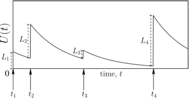
We associate to each user a time-varying, non-negative real valueU(t)that we calluser excitation. The user excitation keeps track of the cumulative effect of the impressions shown to the user, assuming that the impact (deterministic or random) of each impression decays over time. As usually done in many physical systems, and supported by the Ebbinghaus’s model [27], the impact on the user of each impression is assumed to decay exponentially over time, with parameterα, representing in our context the physiological process of forgetting. Parameterαcan be inferred for the specific user, or just estimated from the average behavior of a larger set of users. We assume, for now, that
2
the exact value ofαis known to the system. In Sec. 5.1, we evaluate the impact of an erroneous estimate ofα.
When an impressioniarrives, it increments the excitation byLi. In the simplest case,Li is just a constant, but for greater generality we allow it to be a random variable accounting for various effects related to the user behavior, the environment, etc. For simplicity, we will assume thatLi are i.i.d. positive random variables with the same distribution and that the distribution ofLi has all polynomial moments finite. Without lack of generality, we can assume that user excitation has mean equal to 1, i.e.,E[Li]=1.
Fig. 2 shows an example of the temporal evolution ofU(t)in the case of a user receiving a sequence of four impressions displayed at timesti,i=1. . .4.
0 L1 L3 t1 t2 t3 t4 time,t L2 L4
U
(
t
)
Fig. 2. Example of evolution of user excitationU(t).
By denoting withtthe current time instant and withti the time at which the user has received thei-th previous impression, the current value of user excitation is given by:
U(t)= Õ
i:ti<t
Lie−α(t−ti). (1)
We will considerU(t)to be left continuous. Two different cases for the stimuliLi may take place:
• Perfect excitation information.The Ad Server knows the timestiand the valuesLi. Under
perfect information onLi andα, the system has full knowledge of the instantaneous user excitationU(t). This is an analytically tractable ideal case, in which we can characterize the optimal strategy, thus deriving upper bounds to the system performance.
• Partial excitation information.In this more realistic case, the Ad Server, in addition to
timesti, has inferred a probability distribution overLi, thanks, for example, to detailed tracking of the interaction between the user and the ads displayed.
In our stochastic framework, the user reacts to an impression depending on the history of past impressions. We introduce the probabilityPathat the user performs an action. To emphasize the dependency of such probability on the user excitation and on the impression just received, i.e., the valueLi., we will denote this probability on impressionidisplayed at timeti byPa(U(ti)+Li). We will refer toPa(x):R+→ [0,1]as the user response function, and again assume that this function is known to the system, having been either inferred for the specific user or estimated across a larger set of users. We do not pose particular restrictions to functionPa, e.g., it does not even have to be continuous. However, to avoid trivialities, we always assume thatPa(x) →0 forx→ ∞.
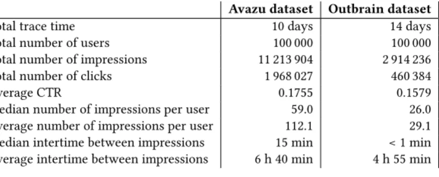
Table 1. Avazu and Outbrain datasets overview.
Avazu dataset Outbrain dataset
Total trace time 10 days 14 days
Total number of users 100 000 100 000
Total number of impressions 11 213 904 2 914 236
Total number of clicks 1 968 027 460 384
Average CTR 0.1755 0.1579
Median number of impressions per user 59.0 26.0
Average number of impressions per user 112.1 29.1 Median intertime between impressions 15 min < 1 min Average intertime between impressions 6 h 40 min 4 h 55 min
3.3 Experimental evidences
We now provide qualitative examples of user response functionPaderived from experimental data, using traces of real advertising systems. Information about user behavior are sensitive, hence all data and traces must be correctly anonymized before processing [32]. The Avazu dataset, publicly available over the Kaggle platform [2], reports the click/no-click actions performed by 9 million anonymized mobile users on on-line ads, over 10 days. Most of the users in the original dataset are not active, with just 1 impression shown during the period. Since we are interested in users that are exposed to many ads, we restrict the analysis to the 100 000 most active users, generating about 11 million impressions. Characteristics of the used dataset are reported in Table 1.3
Assuming, in the absence of further information, thatLi’s are deterministic and equal to 1 we computed the evolution of the shot-noise processU(t)for each user using the impression arrival times trying different values ofα. For each value ofα, we have then evaluated the corresponding empirical user response function4, using the click/no-click information in the trace. Fig. 3(a) reports the empiricalPa, in the case ofα = 0.3, using a uniform binning for the user excitation. We emphasize that, although we display aggregate results for all considered users, each user has been treated independently from the others, by reconstructing his/her specific excitation. The dashed line in the plot shows the best least-square fitting of the experimental data by an exponential function, that we will use later on (Sec. 4.5). Results in Fig. 3(a) reveal a significant correlation between the user response and the user excitation5, suggesting that our methodology can be effectively employed to model and optimize the system (as explained in Sec. 4).
We repeated the same experiment with the Outbrain dataset, also available on the Kaggle platform [4]. The trace contains click/no-click information on roughly 15 million users over a period of 14 days, though again no-clicks have been significantly subsampled to reduce the trace size. In this dataset, most of the users are exposed only to a single burst of very few ads. Again, we restricted our attention to the 100 000 most active users, accounting for approximately 3 million impressions (see Table 1). Fig. 3(b) shows the empiricalPaobtained again forα =0.3. Interestingly, results are similar to those coming from the Avazu dataset. They suggest that, in both datasets, user response is mainly affected by a boredom effect, producing a monotonically decreasing user response function.
3
While the publicly available trace contains all click events, no-click events have been subsampled by Kaggle to limit the trace size, which explains why the observed CTRs are significantly larger than what usually reported.
4
To avoid transient effects, we discarded for each user the first 2/αhours of the reconstructedU(t)process.
5
We obtained similar results for other values ofαaround 0.3, whereas correlation tends to vanish for much smaller (≈0.01) or much larger (≈10) values.
To make our results reproducible and to foster new research on the topic, we decided to make available to the community the used datasets and the software for analyzing them.6
0 20 40 60 80 100 User excitation U 0.06 0.09 0.12 0.15 0.18 0.21 Pa (a) 0 5 10 15 20 25 30 User excitation U 0.08 0.10 0.12 0.14 0.16 0.18 0.20 Pa (b)
Fig. 3. ExperimentalPaobtained from (a) Avazu and (b) Outbrain datasets.
As further evidence of the existence of the boredom effect, in Fig. 4 we show the histogram of the probability that a specific item is clicked at itsn-th appearance (n=1, . . . ,5), given that it has been shown to the same user at leastntimes and has been clicked by the users. Here we consider the same users as before and we focus on a sequence of specific advertisements. We observe that the considered probability drops sharply withn, with only 12% of clicks at the second impression delivery, and 3% of clicks at the third impression delivery. No item was clicked after its 5-th impression delivery to the same user.
In marketing research, it is also common to consider a non-monotonous user response function with a single peak to jointly account for habituation and boredom. An inverted-U shaped function has been justified by Berlyne’s theory of exploratory behavior [7], who first studied the relationship between attractiveness of a stimulus and its familiarity (number of repetitions). Since such a theory
6
Filtered datasets and codes are available at the following public link: https://mplanestore.polito.it:5001/sharing/aSAcHJBtg.
1 2 3 4 5 n 10 3 10 2 10 1 100
Conditioned click probability
Fig. 4. Probability to click an item at itsn-th appearance (n=1, . . . ,5), given that it has been clicked and shown to the same user at leastntimes.
has been largely adopted in marketing research, in our evaluation we will also consider a non-monotonousPa, in addition to a monotonically decreasing function like the simple exponential fitting shown in Figs. 3(a) and 3(b).
At last, we emphasize that, although the way in which we have fitted our model to the Avazu and Outbrain datasets is largely arbitrary, due to intrinsic limitations of the information available in the traces, the main point that we want to make is thatuser response and user excitation are
indeed significantly correlated, at least over appropriate time scales. IfPawere independent, or very weakly correlated withU (e.g., a flat function), there would be no room for any optimization, i.e., no reason to introduce any frequency capping: the best strategy would be to overwhelm the users with ads, exploiting all possible impression opportunities.
3.4 Timeliness of ads delivery
Since tracking and profiling technologies permit designing advertising strategies tailored to indi-viduals, we will focus on just one user, whose profile (interests, navigation habits, response history to past advertisements) is known to the system. In the absence of information about the user (e.g., a new visitor), the system will initially use average characteristics of its known users. We will further assume that candidate ads to be sent to the user are qualitatively similar, i.e., they can be considered to be equally interesting to the user according to its current profile information. Note that the Ad Server (see Fig. 1) has to match candidate ads of the Advertiser with available slots of the Publisher. In the following, we refer to a matched pair (ad+slot) as animpression opportunity.
For such model, we analyze the following scenarios:
• Arbitrary delivery.The system can send impressions to the user at arbitrary time instants.
This assumption provides an upper bound to the system performance. Moreover, it can be considered as a good approximation of systems in which there is abundance of impression opportunities, i.e., when we jointly have (see Fig. 1): i) abundance of slots, meaning that the user is online often enough (as compared to the time-scale of the optimal ad delivery rate); ii) abundance of ads, meaning that new ads arrive at sufficiently large rate, and they are delay-tolerant (i.e., they can be delayed, maintaining equal interest to the user).
• Real-time delivery.Either because of scarcity of slots, or because of scarcity of ads (not
delay-tolerant), the system is forced to select the impressions to send to the user from an online stream of finite rateλ. In particular, we will consider the case in which impression opportunities become available to the system according to a Poisson process of rateλand the system has to make an instantaneous decision on whether to send each impression to the user or not.
• Buffer delivery.This is an intermediate case, which we will explore by simulation, in which
ads arrive at the Ad Server at finite rateλand remain valid for some known time (deterministic or random). Slots are abundant so that ads can be shown to the users at arbitrary times.
Under our assumptions, the profits of an ad-campaign are directly proportional to the CTI, thus our objective will be to maximize such metric under the various scenarios introduced above.
3.5 The baseline SLT strategy
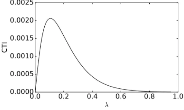
Before diving into the analysis, we propose a baseline frequency capping strategy in the case of partial excitement information and real-time delivery that will be used for comparison in the next sections. We assume impression opportunities arrive according to a Poisson process of rateλand the Ad Server just delivers the impressions to the user as soon as they arrive. FFig. 5 reports the CTI as a function of the arrival rateλ, assumingLi =1∀i,α =0.1, and the monotonically decreasing response functionPa =0.1e−u. Fig. 5 clearly shows that there exists an optimal ad-delivery rate
0.0
0.2
0.4
0.6
0.8
1.0
λ
0.0000
0.0005
0.0010
0.0015
0.0020
0.0025
CTI
Fig. 5. CTI as a function of delivered impression rate of a Poisson process.
maximizing the CTI. We propose a strategy called stateless thinning (SLT), which performs a thinning of the arriving stream of impression opportunities by sending each opportunity to the user with fixed, independent probabilityp. In Appendix A we show that the optimal thinning probabilitypcan be analytically derived. Note that, assumingλlarge enough, as we varypthe above SLT strategy would precisely achieve the performance shown in Fig. 5 (regarding thex-axis as the rate of thinned impressions). Therefore, an optimal choice ofp, possibly by trial and error, would allow us to achieve the maximal value of CTI in Fig. 5.
We argue that this simple SLT strategy, if adopted, could already improve the profits of online campaigns that overwhelm users with uncapped impressions, thus operating on the right portion of the curve shown in Fig. 5. In general the SLT strategy is not optimal, under both arbitrary and real-time delivery scenarios.
We conclude this section with an observation. Under any strictly decreasing user-response (like the one in the example), CTR is maximized under vanishing ad-delivery rate, i.e., by waiting until the user excitationU becomes very small, so that the next opportunity will be accepted with the highest probability. Clearly, so doing one would achieve vanishing CTI, confirming that CTR is not the right metric to consider when maximizing the profit of an ad campaign seeking multiple actions from the user.
4 STRATEGIES WITH PERFECT EXCITEMENT INFORMATION
We start with the case in which the system has full knowledge of the user excitationU(t), i.e., the perfect excitement information case. Let{ti}ibe the sequence of times at which the user is exposed to impression opportunities, i.e., right before the excitation increment due to impression delivery. We observe thatU(ti)is uniquely determined by the triplet(U(ti−1),Li−1,τi), withτi =ti −ti−1. In other words, assumingU(ti−1)to be given,U(ti)is conditionally independent of{U(tj)}j for
j<i−1, wheneverτi is conditionally independent of{τj}j<i,{U(tj)}j<i−1{Lj}j<i−1.
We can thus restrict ourselves to study Markovian policies (i.e., consider policies according to which{τi}isatisfies previous properties), and prove that{U(ti)}iforms an ergodic Markov process overR+(or a compact subset ofR+) under some additional weak assumptions on the distribution ofLiandτi.
Proposition 4.1. Assume that: (i)Li, which represents the increment in the user excitation upon
polynomial moments andτi >δwith probability one, for someδ >0, wheneverU(ti−1)is sufficiently
large. Then{U(ti)}i represents an ergodic Markov process.
Proof. A proof of the ergodicity of{U(ti)}i can be given with standard drift arguments. In-deed,E[U(ti) | U(ti−1)] =E[(U(ti−1)+Li−1)e −ατi] < ( E[U(ti−1)]+E[Li−1])e −α δ = E[U(ti−1)] − E[U(ti−1)](1−e −α δ)+ E[Li−1]e −α δ <
E[U(ti−1)] −1 wheneverE[U(ti−1)]is sufficiently large. □ Being the process ergodic, we can defineπU(u)as the unique stationary distribution of{U(ti)} over a properly defined support. In the following, we study the{U(ti)}iprocess under stationary conditions and denote byU the random variable representing the user excitation at the generic timeti. We also denote byLthe genericLi.
Given the above observations and assumptions, below we derive the optimal Markovian policy under both arbitrary delivery (Sec. 4.1) and real-time delivery (Sec. 4.2) scenarios.
4.1 Arbitrary delivery
Recall that in this scenario the Ad Server can deliver impression opportunities to the user at arbitrary time instants. We will show that in this case the policy that maximizes the CTI is the one that sends a new impression opportunity to the user whenever the excitationU(t)goes back to a fixed, optimal valueθ0, which depends on the response functionPaand the distribution ofLi.
We start by proving the following proposition, which expresses the CTI as the ratio between the average revenue obtained by an impression and the average time between two consecutive opportunities shown to the user.
Proposition 4.2. TheCTIachieved by a Markovian policy with stationary distributionπU(u)is
given by: CTI = αEUEL [Pa(U +L)] EUELlog 1+UL = α ∫ u ∫ lPa(u+l)dFL(l)dπU(u) ∫ u ∫ llog 1+ l u dFL(l)dπU(u) . (2)
Proof. The above result is obtained by applying renewal theory; the proof can be found in
Appendix B. □
Looking at (2), it can be seen that the CTI depends on the selected policy only through the stationary distributionπU(u). Therefore, all the Markovian policies with the same stationary distribution lead to the same performance. In particular, we are interested in the optimal policy associated to π∗ U(u)=arg max πU(u) EUEL[Pa(U +L)] EUELlog 1+ L U
where for now we assume that a maximum exists overπU(u)(its existence is shown below). Next, within the class of Markovian policies, we define a subclass of policies enforcingU(ti)=θ, ∀i, i.e., policies that expose the user to a new impression opportunity whenever the excitation goes back to a given thresholdθ. In the following, we will generally refer to such polices as
threshold-based. For threshold-based policies, the expression of CTI reduces to: CTI= α∫ lPa(θ+l)dFL(l) ∫ llog 1+θl dFL(l) .
1.0 1.5 2.0 2.5 3.0 3.5 4.0 4.5
COV
0.000
0.005
0.010
0.015
0.020
0.025
0.030
CTI
CTI
0.2
0.3
0.4
0.5
0.6
0.7
θ
0θ
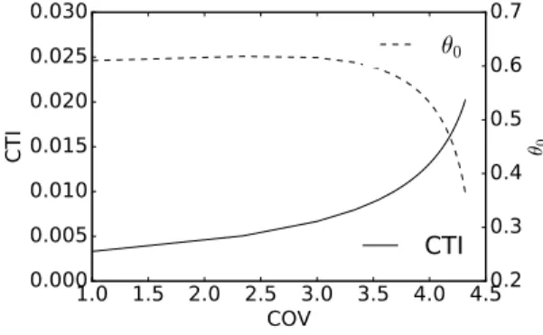
0Fig. 6. Optimal threshold and corresponding CTI as a function of the coefficient of variation of the hyper-exponential distribution ofL.
Theorem 4.3. An optimal Markovian policy is the threshold-based policy using thresholdθ0such
that: θ0=arg max θ ∫ lPa(θ+l)dFL(l) ∫ llog 1+l θ dFL(l) . (3)
Proof. We denote with f(θ) =
∫ lPa(θ+l)dFL(l)andд(θ) = ∫ llog 1+θl dFL(l). Note that clearlyf(θ)andд(θ)are non-negative functions, withд(θ)>0∀θ >0. It can be shown that:
∫ θ f(θ)dπU(θ) ∫ θд(θ)dπU(θ) ≤ f(θ0) д(θ0) . Indeed, ∫ θ f(θ)dπU(θ) ∫ θд(θ)dπU(θ) = ∫ θ[f(θ) −f(θ0)] dπU(θ)+f(θ0) ∫ θ[д(θ) −д(θ0)]dπU(θ)+д(θ0) = f(θ0) д(θ0) © « 1+∫ θ f(θ) f(θ0)− 1 dπU(θ) 1+∫ θ д(θ) д(θ0) −1 dπU(θ) ª ® ® ¬ . Now we get the assertion by proving that
1+ ∫ θ f(θ) f(θ0) −1 dπU(θ) 1+ ∫ θ д(θ) д(θ0) −1 dπU(θ) =1+α 1+β ≤ 1.
Of course the assertion is trivially true ifβ >α, i.e.,α−β ≤0. The latter expression holds since by construction:α−β =∫ θ f(θ) f(θ0)− д(θ) д(θ0) dπU(θ)and, by definition ofθ0, f(θ) f(θ0) − д(θ) д(θ0) = fд((θθ) 0) f(θ) д(θ) − f(θ0) д(θ0) ≤0. Notice thatθ0<∞is a consequence of our assumptions onPaand{τi}i.
□
Fig. 6 shows the impact of the distribution ofL(specifically, the variance ofL) on the optimal threshold and the corresponding maximum CTI. We consider forLa simple hyper-exponential
distribution of the second order, which allows us to vary the coefficient of variation (COV) while keeping the mean fixed to 1. We further assume thatPa=0.1e−uandα=0.1, as in the example of Fig. 5. Interestingly, as the variance ofLincreases, the optimal value of the threshold decreases while the resulting CTI increases. This can be explained as follows: by increasing the coefficient of variation ofL, we observe few (rare) larger and larger spikes ofL, interleaved with many smaller and smaller spikes. While large (rare) spikes ofLquickly fade away thanks to the exponential decay of user excitation, the presence of many small spikes allows the system to sample the user excitation at a lower level, thus yielding larger values of user response.
4.2 Real-time delivery
Recall that in this scenario the system has to make an instantaneous binary decision (selection) of impression opportunities arriving according to a Poisson process of rateλ.
The optimal selection policy can be formalized as a Markov decision process over continuous space. The state of the process is given by the user excitation sampled at the time instants at which a new impression opportunity arrives. At each sampling timetn, two decisionsaare possible: either the opportunity is sent to the user (a=1), or it is discarded (a=0). Thus, the instantaneous reward at the generic sampling timetnis:
R(n,a)=
P
a(U(tn)+Ln) if a=1
0 if a=0
(4)
For tractability, we approximate the above Markov decision process by discretizing the level of user excitation and defining a Markov Chain where thei-th state corresponds to excitation levelUi. So doing, we can apply known results from the theory of stochastic dynamic programming [29, Ch. 5], which allows us to characterize the optimal filtering policy. In particular, Theorem 2.4 in [29, Ch. 5] states that, if the Markov Chain, for any possible policy, includes an ergodic state, the policy that maximizes the average reward is stationary, i.e., the action taken at a given time instant deterministically depends on the current state. Note that, in our system, the state corresponding to any arbitrarily small levelϵof user excitation is ergodic since it can be reached from any other state due to the decaying behavior of the excitation and the fact thatLis assumed to have finite moments.
In general, the optimal policy can be found by solving Belman’s equation [29]:
w+h(n)=max a " R(n,a)+ ∞ Õ j=0 Pij(a)h(j) # , n≥0
whereh(n)is a bounded function,wis a constant representing the average optimal reward and
Pij(a)is the probability to move from stateitoj, given that decisionais made.
By using this approach, we found that in many cases of practical interest the optimal policy is threshold-based: impression opportunities arriving at time instants at whichU(tn) ≤θ∗, whereθ∗ is an optimized threshold, have to be delivered to the user, whereas whenU(tn)>θ∗opportunities have to be discarded. We remark that there are cases in which the optimal policy is not threshold-based, but we found them just in pathological cases with non-continuousPa, and obtaining a negligible gain. We will show one of these counter-examples in Appendix C.
Thus, in the following we will focus on the performance achieved by threshold-based policies. For givenθ, we can compute the stationary distributionπU(u)induced by the corresponding threshold-based policy. Indeed, for real-time delivery, the CTI resulting from a threshold-based
policy can be related toπU(u)as: CTI=λ
∫ θ
0
Pa(u+l)fL(l)dπU(u). LetfU(u)be the probability density function ofU (i.e.,fU(u)=
dπU(u) du ).
Theorem 4.4. Function fU(u)is the only normalized solution (such that∫ fU(u)du=1) of the
integral equation: fU(u)=λ ∫ ∞ 0 e(α−λ)t∫ θ 0 fL(ueα t−x)fU(x)dxdt+λ ∫ ∞ 1 α log(θ u) fU(ueα t)e(α−λ)tdt. Proof. To obtain the stationary distributionπU(u), we derive the Chapman-Kolmogorov equa-tions associated to the Markov process (over continuous space state)Ui =U(ti):
Ui+1=(Ui+Li11[Ui≤θ])e−ατi+1
whereτi+1 =ti+1−ti and the condition in the indicator function accounts for the fact that an impression opportunity is delivered only ifUi ≤ θ. Now, denoted with fU
i(u)the probability
density function ofUi, we can derive an integral equation relatingfU
i(u)to fUi+1(u). To do so, let Vi =(Ui+Li11[U
i≤θ]). By conditioning on the valuexassumed byUi, we have:
fVi(u|x)=fL(u−x)11[x≤θ]+δ(u−x)11[x>θ]
where the first and second term on the right hand side account, respectively, for the case where an impression opportunity is delivered (x ≤θ) and the case where the user excitation is above the threshold. Then, unconditioning, we get:
fVi(u)=
∫ θ
0
fL(u−x)fUi(x)dx+fUi(u)11[u>θ].
Now we can observe that, conditionally overτi+1 =t,Ui+1andVi are deterministically related, beingUi+1=Vie −α t. Therefore,f Ui+1(u |t)=e α tf Vi(ueα t). Then fUi+1(u|t)=e α t∫ θ 0 fL(ueα t −x)fUn(x)dx+eα tfUi(ueα t)11[ueα t>θ].
Finally, unconditioning we get:
fUi+1(u)=λ ∫ ∞ 0 e(α−λ)t∫ θ 0 fL(ueα t−x)fUi(x)dxdt+λ ∫ ∞ 1 αlog(θu) fUi(ueα t)e (α−λ)tdt. (5)
Given the assumption on stationarity, we can impose thatfU
i(u)=fUi+1(u)=fU(u), thus fU(u)is
obtained as the only normalized solution of the stated integral equation. □ 4.3 Buffer-Driven Filtering (BDF) strategy
We now consider the buffer delivery scenario lying in between the extreme cases of arbitrary delivery and real-time delivery. As anticipated in Sec. 3, we assume that, similarly to the arbitrary delivery case, the Ad Server can send impressions to the user at arbitrary time instants (the user is supposed to be permanently exposed to ads), but within a given deadline for each ad. In other words, ads can be buffered for some timeD(deterministic or random) at the Ad Server. We denote byρ =λE[D]the corresponding ‘traffic intensity’. For such intermediate scenario, we propose a heuristic strategy, named buffer-driven filtering (BDF), based on the following idea: whenever there are at least two ads in the buffer, we employ the optimal thresholdθ0of arbitrary delivery. When we have a single ad in the buffer, we employ the optimal real-time thresholdθ∗. Moreover,
we delay the deliver of this single ad until it is close to expire, in order to maximize its acceptance probability. The detailed pseudo-code is provided in Appendix D.
4.4 Numerical evaluation
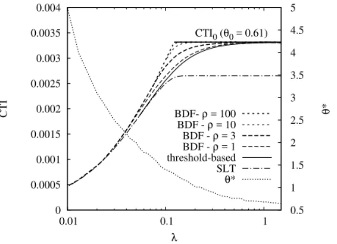
We now compare the performance of the strategies presented in the previous sections. To this end, we consider a scenario in which we fix againα =0.1, whileLis assumed to be exponentially distributed (with mean 1). We consider either a monotonically decreasing response function, or an inverse-U response function. As we vary the arrival rateλof the arriving (Poisson) stream of (candidate) impression opportunities, we compare the CTI achieved by:
• the stateless thinning strategy (SLT), with optimal thinning probabilityp;
• the CTI achievable under arbitrary delivery, hereinafter denoted by CTI0=CTI(θ0), which represents an upper-bound to the system performance (Sec. 4.1);
• the threshold-based real-time strategy, with optimal thresholdθ∗(Sec. 4.2);
• the buffer-driver filtering (BDF) strategy introduced above, for different values of traffic intensityρ. 0 0.0005 0.001 0.0015 0.002 0.0025 0.003 0.0035 0.004 0.01 0.1 1 0.5 1 1.5 2 2.5 3 3.5 4 4.5 5 CTI θ* λ CTI0 (θ0 = 0.61) BDF- ρ = 100 BDF - ρ = 10 BDF - ρ = 3 BDF - ρ = 1 threshold-based SLT θ*
Fig. 7. CTI vs. impression rateλunder various strategies, for monotonically decreasing response function
Pa=0.1e−u.
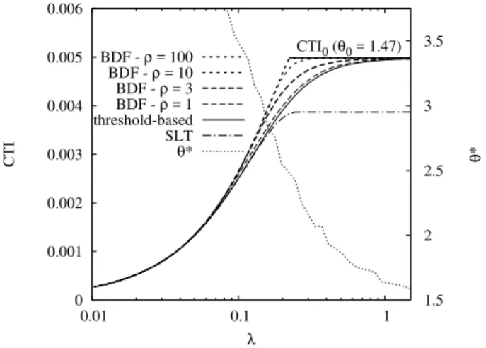
Fig. 7 and Fig. 8 show the CTI achieved by the considered strategies in the case of, respectively, decreasing response functionPa=0.1e−u and inverse-U response functionPa=0.1ue−u. In both figures we also show on the right y axes the value of the optimal thresholdθ∗for the real-time delivery case.
Note that, consistently with what said in Sec. 3.4, the upper bound CTI0provided by arbitrary delivery only makes sense whenλ > λmin, whereλmin is the rate of impression opportunities delivered to the user by the optimal policy. Such minimum rate is given by:
λmin= α ∫ llog 1+ l θ0 dFL(l)
This explains why we show CTI0as an horizontal line starting from the point at whichλ=λmin. Specifically, we have CTI0=0.0033 in the case of Fig. 7, forθ0=0.61, whereas we get CTI0=0.005 in the case of Fig. 8, forθ0=1.47.
0 0.001 0.002 0.003 0.004 0.005 0.006 0.01 0.1 1 1.5 2 2.5 3 3.5 CTI θ* λ CTI0 (θ0 = 1.47) BDF - ρ = 100 BDF - ρ = 10 BDF - ρ = 3 BDF - ρ = 1 threshold-based SLT θ*
Fig. 8. CTI vs. impression rateλunder various strategies, for inverse-U response functionPa=0.1ue−u.
Results are qualitatively similar for both considered user response functions. All strategies tend to achieve similar performance for smallλ, where filtering is not needed and the best choice is to just deliver to the user all arriving impression opportunities.
Asλ increases and filtering becomes effective, some differences arise. The CTI obtained by the threshold-based policy increases withλ, till it saturates to the upper-bound. Note that the corresponding value of optimal threshold in the case of real-time delivery,θ∗, decreases withλ, approachingθ0. The SLT strategy, instead, saturates to a lower value and much earlier than the threshold-based policy. The reason is that SLT is a simpler strategy unaware of the system state, and for largeλcannot do any better than delivering a Poisson stream of opportunities to the user (which is suboptimal).
The performance of the BDF algorithm strongly depends on the traffic intensityρ(note thatρ equals the average buffer occupancy of an M/G/∞queue storing the arriving opportunities). As expected, for large values ofρ(e.g., larger than 10), BDF approaches the upper bound, while for small values ofρ(e.g., smaller than 1) BDF essentially behaves like the real-time delivery strategy. 4.5 Trace-driven results
In Sec. 3.3 we already described a simple way to fit our model to the Avazu and Outbrain traces, assuming fixedL=1 and obtaining an empirical user response function withα =0.3. We now make an additional step, comparing the actual CTI measured on the traces with the CTI resulting from the fitted model. Specifically, for both traces we consider a simple least-square exponential fitting of the user response function (the dashed lines in Figs. 3(a) and 3(b)). Using the actual arrival process of impressions appearing in the traces, we build the excitationU(t)of each user (assuming that users are homogeneous), settingα =0.3 andL=1. We can then obtain the CTI as predicted by the model, and compare it with the actual CTI of the traces. Despite the strong approximations introduced by our methodology (e.g., the least-square fitting, the assumption that users are homogeneous), we found that, for both traces, the CTI predicted by the model closely matches the actual CTI, with a relative error below 5%. This further confirms the validity of the system model introduced in Sec. 3.
We then tried to apply our filtering strategies to the arrival process of ads contained in the traces, in order to achieve possible better CTI. Unfortunately, the arrival rate of impressions in both traces is significantly smaller thanλmin, leaving little room for improvements. For example, we tried the
simple SLT strategy, with a numerically optimized thinning probabilityp. The optimalpturns out to be equal to 1, meaning that SLT does not lead to any improvement. Due to the scarcity of impression opportunities, the arbitrary delivery strategy cannot be applied (λ<λmin). For the same reason, the threshold-based real-time strategy yields only marginal gains (in the order of 1%), since
U(t)very rarely goes above the optimal thresholdθ∗.
When, instead, the BDF strategy is adopted (assumingρ=100), i.e., impressions can be delayed, and thus better spread out over time, we obtained significant improvements in CTI, namely, 7% in the case of the Avazu trace and 24% for the Outbrain trace. This can be explained by the fact that the arrival process of ads in both traces is quite bursty.
In conclusion, we can say that: i) real traces confirm the validity of our model in representing user behavior and predicting the resulting CTI; ii) for moderate values of impression rate, a careful optimization of the times at which impressions are submitted to the user (when this is possible, i.e., when ads can be delayed) can produce significant gains in terms of CTI.
5 ESTIMATION OF THE EXCITATION INFORMATION
We now move to the case in which the Ad Server does not have perfect knowledge of the user excitation at timet,U(t). However, the following information is available to the advertising platform: (i) the time instants at which previous impression opportunities have been delivered to the user (i.e., the sequence{ti}i:ti<t), and (ii) the outcomes{Xi}i:ti<t, of such opportunities (i.e., whether the user has performed a valuable action (Xi =1) or not (Xi =0), on each opportunity). We also assume that the system is aware of the statistics ofLi, ofαand of the user-response functionPa. Notice that if a user is lowly active, i.e., rarely online and rarely clicking on ads, it will be hard to correctly estimate the user peculiar parameters (Pa,α, andLi) and the excitation levelU(t). However, in this scenario, there would be little room for improvement in CTI.
From the above information, the Ad Server can derive an estimateUˆ(t)of the exact value of user excitationU(t), to be used for deciding when/whether to send the next opportunity to the user. In this case of partial excitation information, the estimation ofUˆ(t)can then be used in all the strategies presented in Sec. 4 for solving the different ads delivery scenarios.
The best estimateUˆ(t) is, by construction, given byUˆ(t) = E[U(t) | {ti}i:ti<t,{Xi}i:ti<t}]. Therefore, given the structure ofU(t), we have:
ˆ
U(t)=Õ
ti<t
E[Li | {Xj}tj<t]exp(−α(t−ti)).
It follows that, in order to estimate the user excitation, we have to obtainE[Li | {Xj}t
j<t]. The exact
analysis ofE[Li | {Xj}t
j<t]is fairly difficult. For example, if we ignored the correlation between
Li and{Xj}j
,i, we could computeE[Li |Xi =1]andE[Li |Xi =0]. Then, by standard Bayesian
analysis, in principle the distribution ofLconditioned to the user’s reaction to the offered item could be obtained as:
FL(l |X =1)= ∫l 0 ∫∞ 0 Pa(u+z)dFL(z)dπU(u) ∫∞ 0 ∫∞ 0 Pa(u+z) dFL(z)dπU(u) . and FL(l |X =0)= ∫l 0 ∫∞ 0 ( 1−Pa(u+z))dFL(z)dπU(u) ∫∞ 0 ∫∞ 0 ( 1−Pa(u+z))dFL(z)dπU(u) .
From the above expressions, it would be easy to deriveE[L |X =1]andE[L|X =0], provided thatπU(u)were known, which unfortunately is not.
We therefore adopt a different approach which aims at estimating directly the distributionπ(i)
U (u)
associated with thei-th impression opportunity sent to the user. To this end, we can write a recursive equation which relatesπU(i)(u)toπ(i−
1)
U (u), givenXi.
Let us defineU(ti+)as the user response at timeti+, i.e., right after the excitation increment that occurs upon the delivery of an impression opportunity; more formally,U(ti+)=limt↓t
iU(t). Also,
for brevity, we denote byUi andπU(i)(u), respectively,U(ti+)and the distribution ofU(ti+). Using such notation, we have:
P(Ui <u|Xi =1,Ui−1=y,τi)= P(Ui <u,Xi =1|Ui−1=y,τi) P(Xi =1|Ui−1=y,τi) . with: P(Ui <u,Xi =1|Ui−1=y,τi)= ∫ (u−ui−)+ 0 Pa(u−i +l)dFL(l). whereui−=ye−ατi and(z)+=max(0,z). Furthermore,
P(Xi =1|Ui−1=y,τi)= ∫ ∞ 0 Pa(u−i +l)dFL(l). Therefore, π(i) U (u |Xi =1,τi)=P(Ui <u|Xi =1,τi)= P (Ui <u,Xi =1|τi) P(Xi =1|τi) = ∫∞ 0 P(Ui <u,Xi = 1|Ui−1=y,τi)dπ (i−1) U (y) ∫∞ 0 P(Xi = 1|Ui−1=y,τi)dπ (i−1) U (y) = ∫∞ 0 ∫ l∈[0,(u−ye−α τi)+]Pa(ye −ατi +l)dFL(l)dπ(i− 1) U (y) ∫∞ 0 ∫∞ 0 Pa(ye −ατi +l)dFL(l)dπ(i− 1) U (y) . (6) Similarly, π(i) U (u |Xi =0,τi)=P(Ui <u|Xi =0,τi) = ∫∞ 0 ∫(u−ye−α τi)+ 0 ( 1−Pa(ye−ατi+l))dFL(l)dπ(i−1) U (y) ∫∞ 0 ∫∞ 0 ( 1−Pa(ye−ατi+l))dFL(l)dπ(i−1) U (y) . (7) The above equations can be used to construct at timeti+an estimate ofπ(i)
U (u), givenτi,π(i−1)
U (u)
andXi. Note that, while the information aboutXi is exploited to estimateπ(i)
U (u), the same infor-mation is ignored when the estimate ofπ(i−
1)
U (u)is built. Therefore, a natural refinement of our estimate exploits the information aboutXi to obtain an a-posteriori estimate ofπ(i−
1)
U (u). To this end, we can write a “backward” equation that gives usP(Ui−1 <y,Xi =1|Ui =u,Xi−1,τi). First, observe thatP(Ui−1 <y,Xi =1 |Ui =u,Xi−1,τi)=P(Ui−1 <y,|Ui =u,Xi−1,τi), sinceXi and
Ui−1are conditionally independent, givenUi, andP(Xi =1|Ui =u,Xi−1,τi)=1. Therefore, we have: P(Ui−1<y |,Ui =u,Xi−1,τi)= P(Ui−1 <y,Xi−1 |Ui =u,τi) P(Xi−1 |,Ui =u,τi) . with: P(Ui−1<y,Xi−1=1|Ui =u,τi)= 1 FL(u) ∫ u (u−ye−α τi)+Pa (u−l)eατidFL(l).
Furthermore, P(Xi−1=1|Ui =u,τi)= 1 FL(u) ∫ u 0 Pa (u−l)eατidF L(l) Then we get: π(i−1) U (y |Xi−1=1,τi)=P(Ui−1 <y|Xi−1=1,τi) = ∫∞ 0 ∫u (u−ye−α τi)+Pa (u−l)eατidFL(l)dπ(i) U (u) ∫∞ 0 ∫u 0 Pa (u−l)eατidFL(l)dπU(i)(u) . (8) and similarly: π(i−1) U (y |Xi−1=0,τi)=P(Ui−1 <y|Xi−1=0,τi)= ∫∞ 0 ∫u (u−ye−α τi)+ 1−Pa (u−l)eατi dFL(l)dπ(i) U (u) ∫∞ 0 ∫u 0 1−Pa (u−l)eατi dFL(l)dπ(i) U (u) . (9) We can therefore iterate between ((6) or (7)) and ((8) or (9)), until convergence to a fixed point is reached.
Note that, fromπ(i)
U (u), we can easily obtain the distribution ofU(t)for anyt ∈ (ti,ti+1)since, by construction, we have:U(t)=uie−α(t−ti)and, hence,
P(U(t)<u)=P(Ui <ueα(t−ti))=πU(i)(ueα(t−ti)). In particular, P(U(ti−+1)<u)=P(Ui <ue α(t− i+1−ti))=π(i) U (ueατi+1).
Notice that the methodology presented here could be computationally heavy. In order to reduce its time complexity, integrals could be computed a-priori by discretizing in spaceU and time∆T. 5.1 Numerical results
In the previous section we described a methodology to estimate the user excitationU(t), given the uncertainty on the sequence ofLi. Aiming at showing the performance of this method, hereinafter referred to asFeedback, we exploit (6)–(9) to computeE[U(t)]and use it to decide when/whether to deliver an impression opportunity to the user. We then derive the resulting CTI for both arbitrary and real-time delivery. To this end, we keep the same setting as in Sec. 4.4, i.e.,α =0.1,Lexponentially distributed with mean 1, andPa =0.1e−u; also, we setλ =1 in the real-time delivery case. We compareFeedbackto a simpler approach, calledFixed-L, according to which the evolution ofU(t) is estimated by assumingLto be deterministic (equal to 1).
In the arbitrary delivery scenario, we apply the optimal threshold-based policy and compute the error in the estimate of the user excitation and the consequent loss in terms of CTI with respect to the case where perfect information is available (CTI0). Fig. 9 depicts the average value of such relative loss and highlights thatFeedbackgets closer to the performance achieved in the presence of perfect information.
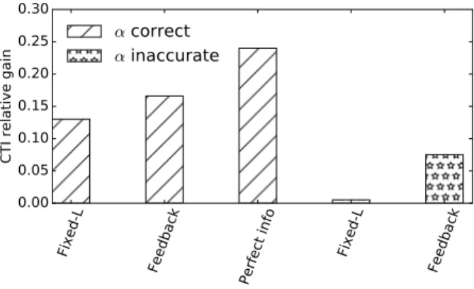
In the case of real-time delivery, we apply the threshold-based, real-time strategy and we report the relative gain we obtain with respect to the SLT method with optimalp. Fig. 10 depicts such a gain, along with the results achieved when perfect knowledge ofU is available. Again,Feedback better approximates the case of perfect information and improves the SLT performance by almost 17%.
Then we assume that the Ad Server has inaccurate knowledge of the decay rateα of user excitation, namely, it underestimatesα by 50%. Consequently, the Ad Server will compute an inaccurate value of the threshold, hence it will expose the user to impressions at non-optimal values of user excitation. The performance ofFixed-LandFeedbackin such scenario is illustrated in Fig. 9 and 10. As expected, the performance decreases with respect to the case in which the exactαis known; however,Feedbackcan better cope with the incorrect knowledge ofαsince it is able to partially compensate the errors by exploiting the information from user response.
Fixed-L
Feedback
Fixed-L
Feedback
0.00
0.05
0.10
0.15
0.20
0.25
CTI relative loss
α
correct
α
inaccurate
Fig. 9. Relative CTI loss in arbitrary delivery scenario, under different approximations ofU.
Fixed-L
Feedback
Perfect info
Fixed-L
Feedback
0.00
0.05
0.10
0.15
0.20
0.25
0.30
CTI relative gain
α
correct
α
inaccurate
Fig. 10. Relative CTI gain in real-time delivery scenario, under different approximations ofU.
6 DISCUSSION AND CONCLUSIONS
In this work we have explored the novel problem of maximizing the number of actions per time unit of a user subject to impressions. Although our analysis relies on a specific user behavioral model, traces of real advertising systems have confirmed the existence of significant correlations between the click probability and the history of impressions shown to the user, which are well captured by our approach. Indeed, by fitting the parameters of the model on the considered traces, we have been
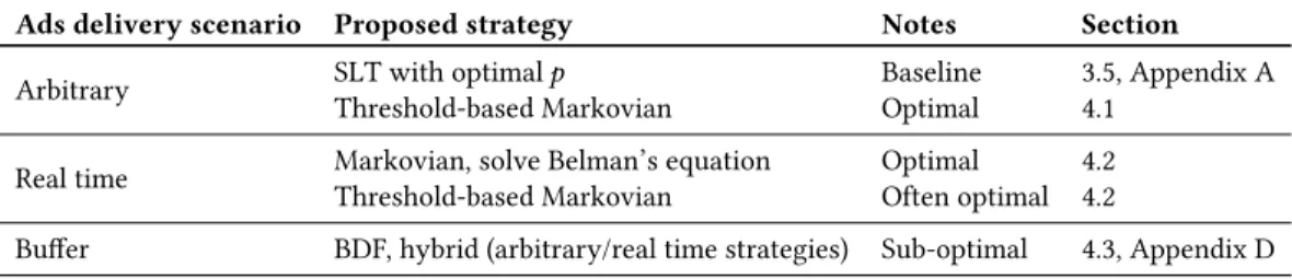
Table 2. Strategies for different delivery scenarios. All the strategy can be applied with perfect or partial excitation information.
Ads delivery scenario Proposed strategy Notes Section
Arbitrary
SLT with optimalp Baseline 3.5, Appendix A
Threshold-based Markovian Optimal 4.1
Real time
Markovian, solve Belman’s equation Optimal 4.2 Threshold-based Markovian Often optimal 4.2
Buffer BDF, hybrid (arbitrary/real time strategies) Sub-optimal 4.3, Appendix D
able to accurately predict the CTI resulting from the temporal sequence of impressions appearing in the traces. More importantly, the model has allowed us to optimize the sequence of impressions itself, achieving significant gains in terms of CTI (and thus in terms of profits). In Table 2, we summarize the proposed strategies for the different delivery scenarios and refer to the Sections where they were presented. All the strategies can be applied even in case of partial excitation information, by estimating the excitation with the Feedback strategy presented in Sec. 5.
As a first step in this new research problem, our analysis has adopted several simplifying assumptions which also have important limitations, as we briefly discuss below suggesting directions for future work. First, we have assumed that candidate impressions are homogeneous (i.e., they are qualitatively identical). A natural extension of our analysis would be to consider heterogeneous impressions, for example divided into different classes having their own arrival rate and user response function. In this case the solution should control the cumulative excitation received by the user. Second, for analytical tractability we have often assumed that the arrival process of impression opportunities is Poisson. Since the activity patterns of a user might not be well described by a simple Poisson process [31], it would be desirable to extend the analysis to more realistic processes, possibly taking into account the on-off nature (sessions) of user exposure. Third, it would be interesting to perform a wider sensitivity analysis on the various parameters of the model, to better assess the impact of incomplete information about the user characteristics. At last, in the real world a user is usually exposed to several competing Ad Servers and ad campaigns, and its response to them is typically not independent, but driven by cumulative effects. A game-theoretic approach would be appropriate to analyze such competition scenario.
ACKNOWLEDGMENTS
This work has been partially supported by the SmartData@PoliTO center on Big Data and Data Science and by the European Union Horizon 2020 Research and Innovation programme under Grant Agreement No. 871370.
REFERENCES
[1] Adwords help: Frequency capping (website). https://support.google.com/google- ads/answer/117579. Accessed July
2018.
[2] Avazu dataset. https://www.kaggle.com/c/avazu- ctr- prediction. Accessed July 2018.
[3] Iab’s internet advertising revenue report (website). https://www.iab.com/wp- content/uploads/2019/05/
Full- Year- 2018- IAB- Internet- Advertising- Revenue- Report.pdf . Accessed September 2019.
[4] Outbrain dataset. https://www.kaggle.com/c/outbrain- click- prediction. Accessed July 2018.
[5] E. Altman. Game theoretic approaches for studying competition over popularity and over advertisement space in
[6] K. Bawa. Modeling inertia and variety seeking tendencies in brand choice behavior.Marketing Science, 9(3):263–278, 1990.
[7] D. Berlyne.Conflict, Arousal and Curiosity. McGraw-Hill, 1960.
[8] J. T. Cacioppo and R. E. Petty. Effects of message repetition and position on cognitive response, recall, and persuasion.
Journal of Personality and Social Psychology, 37(1):97–109, 1979.
[9] B. J. Calder and B. Sternthal. Television commercial wearout: An information processing view.Journal of Marketing
Research, 17(2):173–186, May 1980.
[10]H. Cao, E. Chen, J. Yang, and H. Xiong. Enhancing recommender systems under volatile userinterest drifts. In
Proceedings of the 18th ACM Conference on Information and Knowledge Management, CIKM ’09, pages 1257–1266, New York, NY, USA, 2009. ACM.
[11]O. Celma and P. Herrera. A new approach to evaluating novel recommendations. InProceedings of the 2008 ACM
Conference on Recommender Systems, RecSys ’08, pages 179–186, New York, NY, USA, 2008. ACM.
[12]J. Chen and J. Stallaert. An economic analysis of online advertising using behavioral targeting.MIS Q., 38(2):429–450,
June 2014.
[13]P. Cremonesi, F. Garzotto, S. Negro, A. Papadopoulos, and R. Turrin. Comparative evaluation of recommender system
quality. InCHI ’11 Extended Abstracts on Human Factors in Computing Systems, pages 1927–1932, New York, NY, USA,
2011. ACM.
[14]A. Das Sarma, S. Gollapudi, R. Panigrahy, and L. Zhang. Understanding cyclic trends in social choices. InProceedings
of the Fifth ACM International Conference on Web Search and Data Mining, WSDM ’12, pages 593–602, New York, NY, USA, 2012. ACM.
[15]Y. Ding and X. Li. Time weight collaborative filtering. InProceedings of the 14th ACM International Conference on
Information and Knowledge Management, CIKM ’05, pages 485–492, New York, NY, USA, 2005. ACM.
[16]M. Elahi, F. Ricci, and N. Rubens. A survey of active learning in collaborative filtering recommender systems.Computer
Science Review, 20:29 – 50, 2016.
[17]P. Farris, B. Neil, P. Phillip, and R. David.Marketing Metrics: The Manager’s Guide to Measuring Marketing Performance.
Pearson Education, 2016.
[18]D. G. Goldstein, R. P. McAfee, and S. Suri. The cost of annoying ads.SIGecom Exch., 13(2):47–52, Jan. 2015.
[19]N. Gupta, A. Das, S. Pandey, and V. K. Narayanan. Factoring past exposure in display advertising targeting. In
Proceedings of the 18th ACM SIGKDD International Conference on Knowledge Discovery and Data Mining, KDD ’12, pages 1204–1212, New York, NY, USA, 2012. ACM.
[20]K. Kapoor, K. Subbian, J. Srivastava, and P. Schrater. Just in time recommendations: Modeling the dynamics of boredom
in activity streams. InProceedings of the Eighth ACM International Conference on Web Search and Data Mining, WSDM
’15, pages 233–242, New York, NY, USA, 2015. ACM.
[21]Y. Koren. Collaborative filtering with temporal dynamics. InProceedings of the 15th ACM SIGKDD International
Conference on Knowledge Discovery and Data Mining, KDD ’09, pages 447–456, New York, NY, USA, 2009. ACM.
[22]T. Q. Lee, Y. Park, and Y.-T. Park. A time-based approach to effective recommender systems using implicit feedback.
Expert Syst. Appl., 34(4):3055–3062, May 2008.
[23]W. Lu, S. Ioannidis, S. Bhagat, and L. V. Lakshmanan. Optimal recommendations under attraction, aversion, and social
influence. InProceedings of the 20th ACM SIGKDD International Conference on Knowledge Discovery and Data Mining,
KDD ’14, pages 811–820, 2014.
[24]X. Lu, X. Zhao, and L. Xue. Is combining contextual and behavioral targeting strategies effective in online advertising?
ACM Trans. Manage. Inf. Syst., 7(1):1–20, Feb. 2016.
[25]A. Maksai, F. Garcin, and B. Faltings. Predicting online performance of news recommender systems through richer
evaluation metrics. InProceedings of the 9th ACM Conference on Recommender Systems, RecSys ’15, pages 179–186,
New York, NY, USA, 2015. ACM.
[26]S. M. McNee, J. Riedl, and J. A. Konstan. Being accurate is not enough: How accuracy metrics have hurt recommender
systems. InCHI ’06 Extended Abstracts on Human Factors in Computing Systems, pages 1097–1101, New York, NY, USA,
2006. ACM.
[27]J. M. J. Murre and J. Dros. Replication and Analysis of Ebbinghaus’ Forgetting Curve.PLOS ONE, 10(7), 07 2015.
[28]C. Rohrer and J. Boyd. The rise of intrusive online advertising and the response of user experience research at yahoo!
InCHI ’04 Extended Abstracts on Human Factors in Computing Systems, pages 1085–1086, New York, NY, USA, 2004. ACM.
[29]S. Ross.Introduction to Stochastic Dynamic Programming. Academic Press, 1995.
[30]J. Shanahan and D. den Poel. Determining optimal advertisement frequency capping policy via markov decision
processes to maximize click through rates. InProceedings of NIPS Workshop: Machine Learning in Online Advertising,
[31]L. Vassio, M. Mellia, F. Figueiredo, A. P. Couto da Silva, and J. M. Almeida. Mining and modeling web trajectories from
passive traces. In2017 IEEE International Conference on Big Data (Big Data), pages 4016–4021, Dec 2017.
[32]L. Vassio, H. Metwalley, and D. Giordano. The exploitation of web navigation data: Ethical issues and alternative
scenarios. In F. D’Ascenzo, M. Magni, A. Lazazzara, and S. Za, editors,Blurring the Boundaries Through Digital
Innovation, pages 119–129, Cham, 2016. Springer International Publishing.
[33]R. W. Wolff.Stochastic modeling and the theory of queues. Pearson College Division, 1989.
[34]J. Yan, N. Liu, G. Wang, W. Zhang, Y. Jiang, and Z. Chen. How much can behavioral targeting help online advertising?
InWWW ’09, pages 261–270, New York, NY, USA, 2009. ACM. A OPTIMAL SLT UNDER POISSON STREAM
LetMU(θ)=EU[eθU(tn)]the moment generating function associated to the stationary distribution ofU(tn). Since{tn}n is a Poisson process, we haveMU(θ)=EU[eθU(0)], since by PASTA we can consider any arbitrary time instant (namely, 0). Now, by construction:
U(0)=
Õ tn∈(−∞,0)
Lneα tn
We also define the truncated version:
UT(0)=
Õ tn∈[−T,0)
Lneα tn
The moment generating function ofUT(0), denoted byMT
U, can be easily obtained by conditioning on the number of points of{tn}that fall in[−T,0). Therefore, we can exploit the following property of Poisson processes: conditionally over their number, the non-ordered points,Zi, of a Poisson process falling over a finite interval are uniformly and independently distributed. It follows that:
MT U(θ |m)=E h eθÍm i=1Lieα Zi i =E " m Ö i=1 eθ Lieα Zi # =Eeθ L1eα Z1 m . (10) with: E h eθ L1eα Z1 i = 1 T ∫ 0 −T ∫ le θleα z dFL(l).dz Therefore, MT U(θ |m)= 1 T ∫ 0 −T ∫ le θleα z dFL(l)dz m . and, unconditioning: MT U(θ)= ∞ Õ m=0 1 T ∫ 0 −T ∫ le θleα z dFL(l)dz m (λpT)m m! e −λpT =exp −λpT +λp ∫ 0 −T ∫ le θleα z dFL(l)dz =exp −λp ∫ 0 −T ∫ l (1−eθle α z )dFL(l)dz . Then forT → ∞, we get:
MU(θ)=exp −λp ∫ 0 −∞ ∫ l (1−eθle α z )dFL(l)dz =exp −λp ∫ ∞ 0 ∫ l( 1−eθle −α z )dFL(l)dz . (11)
Observe that, if we assumeLto have a compact support, then forz → ∞,le−α z → 0, hence, exp(θle−α z)=1+θle−α z+o(e−α z). In other words, the integrand function decays to 0 exponentially fast asz→ ∞.
Due to the complexity of (11), we aim at deriving a simpler expression forMU(θ). To this end, for everyT >0, we write:
∫ T 0 ∫ l 1−eθle −α z dFL(l)dz= =∫ T 0 ∫ l 1− ∞ Õ k=0 (θl)k k! e −kα z ! dFL(l)dz = ∞ Õ k=1 θk k! ∫ T 0 e−kα z dz ∫ ll kdF L(l) = ∞ Õ k=1 θk k! 1−e−kαT kα EL[Lk] Thus, ∫ ∞ 0 ∫ l( 1−ele −α z )dFL(l)dz= = lim T→∞ ∞ Õ k=1 θk k! 1−e−kαT kα EL[Lk] = ∞ Õ k=1 θk k! EL[Lk] kα (12) We therefore obtain: MU(θ)=exp −λp ∞ Õ k=1 θk k! EL[Lk] kα ! (13)
From (13), it is then straightforward to derive the stationary distributionπU(u), which will depend onp. Since the filtered arrival process is still Poisson, it follows that the optimal policy can be found by replacing the expression ofπU(u)in the revenue and by optimizing the latter with respect top. B PROOF OF PROPOSITION 1
First note that, under an ergodic Markovian policy, the evolution of the user excitation is Markovian. Furthermore, it can be seen that, under any ergodic policy with stationary distributionπU(u), the evolution of the user excitation over continuous time forms a regenerative process. This because choosing an arbitrary ˜usuch that 0<πU(u˜)<1 and defining with{σ˜i}i the sequence of times at whichU(t)=u˜, we can show that{σ˜i}i forms a non defective sequence of stopping times for the continuous time processU(t)(i.e.,E[σ˜i −σ˜i−1]<∞). Indeed, let us defineSu˜ as the set of states in correspondence of whichU(t) ≤u˜andSu˜ as the complementary set corresponding to values
U(t) >u˜. Then we can observe that: i) by ergodicity, the sequence of times{σi}i, at which the system enters a state inS
˜
u from a stateSu˜ forms a non defective sequence; ii) by construction, {σi}i ⊆ {σ˜i}i, therefore{σ˜i}i is non defective.
It follows that we can apply standard Reward-Renewal results [33], according to which the average revenue if given by
R=E[Pa(U +L)] E[τ]