D
ISSERTATION
SUBMITTED TO THE
COMBINED FACULTY FOR THENATURAL SCIENCES AND FOR MATHEMATICS
OF THE
RUPERTO-CAROLA UNIVERSITY OF HEIDELBERG, GERMANY
FOR THE DEGREE OF
DOCTOR OF NATURAL SCIENCES
PUT FORWARD BY
Diplom-Physiker Christoph-Nikolas Straehle Born in Heidelberg
Interactive Segmentation,
Uncertainty and Learning
Abstract
Interactive segmentation is an important paradigm in image processing. To minimize the number of user interactions (“seeds”) required until the result is correct, the computer should actively query the human for input at the most critical locations, in analogy to active learning. These locations are found by means of suitable uncertainty measures. I propose various such measures for the watershed cut algorithm along with a theoretical analysis of some of their properties in Chapter 2.
Furthermore, real-world images often admit many different segmentations that have nearly the same quality according to the underlying energy function. The diversity of these solutions may be a powerful uncertainty indicator. In Chapter 3 the crucial prerequisite in the context of seeded segmentation with minimum spanning trees (i.e. edge-weighted watersheds) is provided. Specifically, it is shown how to efficiently enumerate the k smallest spanning trees that result in differentsegmentations.
Furthermore, I propose a scheme that allows to partition an image into a previously unknown number of segments, using only minimal supervision in terms of a few must-link and cannot-link annotations. The algorithm presented in Chapter 4 makes no use of regional data terms, learning instead what constitutes a likely boundary between segments. Since boundaries are only implicitly specified through cannot-link constraints, this is a hard and nonconvex latent variable problem. This problem is adressed in a greedy fashion using a randomized decision tree on features associated with interpixel edges. I propose to use astructuredpurity criterion during tree construction and also show how a backtracking strategy can be used to prevent the greedy search from ending up in poor local optima.
The problem of learning a boundary classifier from sparse user annotations is also considered in Chapter 5. Here the problem is mapped to a multiple instance learning task where positive bags consist of paths on a graph that cross a segmentation boundary and negative bags consist of paths inside a user scribble.
Multiple instance learning is also the topic of Chapter 6. Here I propose a multiple instance learning algorithm based on randomized decision trees. Experiments on the typical benchmark data sets show that this model’s prediction performance is clearly better than earlier tree based methods, and is only slightly below that of more expensive methods.
Finally, a flow graph based computation library is discussed in Chapter 7. The presented library is used as the backend in a interactive learning and segmentation toolkit and supports a rich set of notification mechanisms for the interaction with a graphical user interface.
Interaktive Segmentierung ist ein wichtiger Bereich in der Bildverarbeitung. Hierbei ist es w¨unschenswert die Anzahl der Benutzerinteraktionen zu minimieren, die gebraucht werden um ein gew¨unschtes Ergebnis zu erzielen. Um das zu erreichen, sollte der Computer den Benutzer an den problematischsten Stellen, in Analogie zum aktiven Lernen, nach zus¨atzlichen Eingaben fragen. Solch problematische Stellen in der Segmentierung k¨onnen durch geeignete Unsicher-heitsmaße lokalisiert werden. In Kapitel 2 schlage ich verschiedene UnsicherUnsicher-heitsmaße f¨ur den watershed cut Algorithmus vor.
Oftmals haben viele verschiedene Segmentierungen nahezu die gleiche Energie bez¨uglich des Optimierungsproblems. Die Unterschiede dieser energetisch nahezu gleichwertigen Seg-mentierungen k¨onnen ein aussagekr¨aftiges Unsicherheitsmaß sein. In Kapitel 3 pr¨asentiere ich einen Algorithmus, welcher die k g¨unstigsten watershed cut Segmentierungen enumerieren kann. Damit wird die Vorraussetzung zur Analyse dieser Segmentierungen geschaffen.
Des Weiteren schlage ich einen Algorithmus vor, welcher es erlaubt ein Bild in eine vorher unbekannte Anzahl von Segmenten zu partitionieren. Dabei benutzt der Algorithmus nur sehr schwache Annotationen in Form von einigen must-link und cannot-link Angaben. Der in Kapi-tel 4 vorgesKapi-tellte Algorithmus nutzt keine lokalen Datenterme sondern lernt direkt was eine wahrscheinliche Grenzfl¨ache zwischen Objekten ist. Da die Grenzfl¨achen nur implizit durch die cannot-link Angaben spezifiziert werden, ist dies ein schwieriges und nicht konvexes Prob-lem. Ich schlage hierzu einen randomisierten Entscheidungsbaum vor, welcher ein strukturiertes Lernkriterium beim Aufbau nutzt und dabei auf Zwischenpixel-Kanten arbeitet. Eine Backtrack-ingstrategie hilft zu verhindern, dass ein schlechtes lokales Optimum gefunden wird.
Das gleiche Problem – einen Grenzfl¨achenklassifikator ausgehend von schwachen Benutzer-annotationen zu lernen – wird auch in Kapitel 5 betrachtet. Das Problem wird auf ein Multiple Instance Lernproblem zur¨uckgef¨uhrt. Hier bestehen positive Taschen aus Pfaden im Graph, die eine Grenzfl¨ache schneiden und negative Taschen aus Pfaden innerhalb einer Benutzerannota-tion.
Das Multiple Instance Lernverfahren ist auch Thema in Kapitel 6. Hier schlage ich einen Mul-tiple Instance Lernalgorithmus basierend auf randomisierten Entscheidungsb¨aumen vor. Exper-imente auf den typischen Benchmarkdatens¨atzen zeigen, dass der Algorithmus etwas schlechter als teurere Methoden abschneidet aber bessere Ergebnisse liefert als alle existierende Ans¨atze, die auch auf Entscheidungsb¨aumen aufbauen.
Schlussendlich wird in Kapitel 7 die datenflussgraphbasierte Softwarebibliothek lazyflow vorgestellt. Die Softwarebibliothek wird als Basis f¨ur ilastik, das interaktive lern und segmen-tier toolkit benutzt, und unterst¨utzt einen großen Satz an Benachrichtigungsmechanismen zur Interaktion mit einer graphischen Benutzeroberfl¨ache.
Contents
1 Introduction 3
1.1 Interactive segmentation . . . 3
1.2 Watershed . . . 5
1.3 Graphs . . . 6
1.4 Minimum spanning trees . . . 6
1.5 Watershed cuts and minimum spanning trees . . . 7
1.6 Watershed edge weights . . . 8
1.7 Decision trees . . . 8
1.8 Thesis overview . . . 10
2 Watershed uncertainty 11 2.1 Introduction . . . 11
2.2 Background and related work . . . 13
2.3 Uncertainty measures for watershed cuts . . . 14
2.3.1 Watershed cuts and minimum spanning trees . . . 14
2.3.2 Link instability via minimum perturbations . . . 15
2.3.3 Correctness of algorithm 2.3.2.1 . . . 15
2.3.4 Uncertainty from stochastic graphs . . . 16
2.3.5 #P-hardness of stochastic watershed cut problem . . . 17
2.4 Evaluation . . . 20
2.4.1 Robot user . . . 20
2.4.2 Experiments . . . 21
2.5 Conclusion . . . 22
3 Enumerating the k best segmentation changing spanning trees 25 3.1 Introduction . . . 25
3.2 Related work . . . 26
3.4 Gabow’s algorithm for the k smallest spanning trees . . . 27
3.5 Enumerating changing segmentations . . . 27
3.5.1 Algorithm correctness . . . 30
3.6 Enumerating diverse segmentations . . . 31
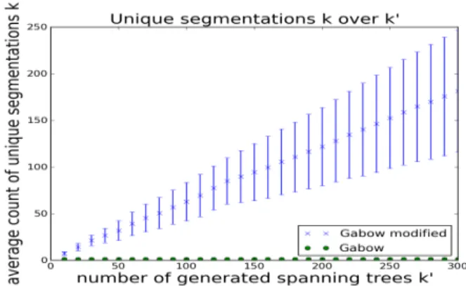
3.7 Experiments . . . 32
3.8 Conclusion . . . 33
4 Image partitioning using structured decision trees 35 4.1 Introduction . . . 35
4.1.1 Related work . . . 37
4.2 Problem definition and objective function . . . 38
4.2.1 Overview: global optimization using decision trees . . . 38
4.2.2 Decision tree building algorithm . . . 40
4.2.3 Backtracking for greedy global decision trees . . . 41
4.2.4 Decision tree prediction algorithm . . . 42
4.3 Experiments . . . 43
4.4 Conclusion . . . 44
5 Multiple instance based edge learning 49 5.1 Introduction . . . 49
5.2 Edge learning as a MIL problem . . . 50
5.3 Experimental evaluation . . . 52
5.4 Conclusion . . . 53
6 Multiple instance optimized random forest 55 6.1 Introduction . . . 55
6.2 Related Work . . . 56
6.3 Decision trees . . . 57
6.4 Random forests . . . 58
6.5 Multi-instance tree learning . . . 58
6.5.1 Tree regularization and weight redistribution . . . 60
6.5.2 Inside/outside split concepts . . . 60
6.5.3 Forest vote bias correction . . . 62
6.5.4 Forest response optimization . . . 62
6.6 Experiments . . . 63
6.6.1 Drug activity prediction . . . 64
6.6.2 Image classification . . . 64
6.6.3 Influence of proposed extensions . . . 64
6.6.4 Discussion . . . 65
Contents
7 Lazyflow: flow graph based computation framework 69
7.1 Related work . . . 71
7.2 Lazyflow operators . . . 72
7.3 Lazyflow slots . . . 75
7.4 Lazyflow requests . . . 78
7.5 Higher level slots . . . 80
7.6 The OperatorWrapper . . . 82 7.7 Composite operators . . . 83 7.8 Summary . . . 84 8 Conclusion 85 List of Publications 87 Bibliography 89
Acknowledgments
I want to thank Prof. Dr. Fred A. Hamprecht for supervising me during the time that has led to this thesis. Already during my master thesis Prof. Hamprecht introduced me to the interesting field of pattern recognition. His research group – Multidimensional Image Processing – has always been a great group of friendly, helpful, knowledgeable and fun people. Secondly, i want to express my gratidude to Prof. Dr. Andrzejak who took the burden of being my second advisor and the time to delve into this project. I also want to thank Dr. Ullrich K¨othe for all his expertise and help throughout the years. With my colleagues I have spent countless hours on programming, bug fixing and discussions while working on the ilastik project. I will always remember the countless tablesoccer matches i have lost to Christoph Decker. Bernhard Kausler has pushed me to write cleaner code. Thorben Kr¨ogers amazing C++ skills always impressed me. Together with Christoph Sommer, Anna Kreshuk, Luca Fiaschi, Martin Schiegg and Stuart Berg we have worked towards a ilastik release. I also wish to thank all my other colleagues, in particular Thorsten Beier, Xinghua Lou, Ferran Diego, Melih Kandemir, Burcin Erocal, Kemal Eren, Philipp Hanslovsky, Robert Walecki, Buote Xu, Ben Heuer, Chong Zhang, Niko Krasowski as well as Carsten Haubold. Furthermore i wish to thank Barbara Werner, Evelyn Wilhem, and Ole Hansen for their support in all administrative affairs. Im also grateful for Oliver Petra and Kai Karius support in writing some lazyflow operators. Finally, i am deeply indebted to my Parents Luise and Wolfgang Straehle and my girlfriend Jil Molitor for supporting me in any possible way throughout these years.
Chapter 1
Introduction
1.1 Interactive segmentation
Interactive segmentation is an important paradigm in image processing. It allows to partition an image into components under the supervision of a human labeler. Such functionality is tremen-dously useful for example in life sciences where biologists need to extract and measure objects of interest from microscopic images. The most basic interactive segmentation method consists of a drawing application which the user can use to segment an image by labeling the individ-ual image parts. This manindivid-ual segmentation process is slow and tedious, especially so for 3D datasets. Over the years many algorithms have been developed that help the user in segmenting image data. These algorithms speed up the segmentation process since they rely only on sparse annotations instead of the dense image labeling. The sparse annotations are used as a start-ing point for some kind of region growstart-ing procedure which stops either at a discernible image boundary or when two different regions start to overlap.
One such segmentation method are theactive contourbased methods such as [26, 27, 137]. In these methods, the evolving estimate of the structure of interest is represented by one or more contours. An evolving contour is a closed surface that evolves over time according to a partial differential equation (PDE). The evolution of the PDE is steered by internal and external forces which act on the normal vector of the closed contour. Internal forces can for example enforce a low curvature of the contour, while external forces usually encode image information and depend on the image location and content at the contour at a time.
Another important line of work arevariational methodsfor image segmentation such as [120]. These methods minimize an energy functional
E(u) = Z Ω g(x)|∇u|dΩ + Z Ω λ(x)|u−f|dΩ, u∈[0,1]
where the outputu = 1 corresponds to a foreground image part andu = 0to a background image part. The data fidelity termλ(x)|u−f|enforces (depending onλ(x)) that the classifier
Figure 1.1: Interactive segmentation illustration. The left picture shows a image from the BSD300 [85] segmentation database and a set of foreground and background seeds a user might give. The right picture shows a potential segmentation result. The task of interactive segmenta-tion algorithms is to produce a result close to the right picture with minimal supervision.
prediction f is obeyed. g(x)|∇u| is the infamous total variation (TV) norm and enforces a smooth surface and small surface area of the foreground-background transition ofu.
Variational methods treat the image spaceΩas a continous domain. In contrast to thisgraph based interactive segmentation methodsdiscretize the domain into a grid graph. Still, the un-derlying principle for interactive segmentation algorithms is the same: an energy function is minimized that consists of a data fidelity term, also called unary potential and a boundary length cost term that is similar to the total variation term. Some of the most important seeded seg-mentation methods on graphs can be unified in terms of thepower-watershedframework [33]. It defines a segmentation as a labeling of a graphG(V, E), where the optimal labelingxminimizes an energy function E(x,w) = X vi∈V w0p,ikxikq+wp1,ik1−xikq +X eij∈E wijpkxi−xjkq (1.1)
xi ∈ L is the label associated with nodevi ∈ V,xis the vector of all label assignments, and
wi, wij are node and edge weights, respectively. The first sum thus measures compatibility of the labeling with a given region model, whereas the second sum enforces smoothness of the solution. For different exponents, the power watershed specializes to the watershed cut algorithm (p → ∞,q finite, [35]), the random walker (pfinite,q = 2, [50]) and an Ising-type Markov random field amenable to graph-cut segmentation (pfinite,q = 1, [18]). A number of coarse-grained [29], pre-computed [51] or warm-started [62] strategies have been suggested to speed up the response to user input for some of the methods.
1.2 Watershed
which can be computed in linear time in the number of pixels. Even when not using the specialized algorithm presented in [35] the computation is still extremely fast as it only re-quires the computation of a minimum spanning forest, or, in an augmented graph a minimum spanning tree computation. Despite of its age, the watershed algorithm is topic of current re-search and is a cornerstone of image processing, especially in 3D and 4D image processing [57, 36, 83, 13, 75, 60, 34]. In this thesis we use the watershed cut algorithm as a basis due to its favorable runtime requirements. The low computational complexity of a minimum spanning tree computation makes this algorithm applicable to large 3D datasets [114, 34, 83, 36]. In ad-dition it was shown that the watershed cut is a very suitable algorithms for some the datasets considered in this thesis [114].
1.2 Watershed
The watershed transform was first introduced for image processing by Digabel and Lantu´ejoul [40] in 1978. Since then many different motivations and algorithms have been proposed which are excellently summarized in [104]. The underlying principle is always similar and centered around the behavior of a drop of water on a topological surface. The image is treated as a height map, with bright pixels corresponding to high elevations and dark pixels corresponding to low elevations. Then, starting from the local minima the topological surface is flooded with water and so called dams or watershed lines are built where water from two different minima meets [124]. Another approach [14] is to look at a drop of water that falls onto the surface and flows along the path of steepest descent to a local minimum. From this viewpoint stems the notion of catchment basinswhich are separated by watershed lines, i.e. the lines from which the drop of water can flow to at least two different minima. The above algorithms treat the problem on a pixel grid graph where the input is a height-map on thenodesof the pixel grid graph, resulting in a so callednode-weighted watershed. Another approach is to look at a height-map associated with theedges of the pixel-grid graph which results in a so called edge-weighted watershed. This approach has been pursued in [35]. The authors show that this edge-weighted watershed is equivalent to a minimum spanning forest computation where the individual trees represent the different local minima or catchment basins. Flooding an image height map or an edge weighted graph from local minima is an unsupervised segmentation paradigm. The watershed however can also be used in a supervised fashion suitable for interactive segmentations. In this setting the algorithm behaves in the same way but starts from a different set of seeds. Instead of associating each local minimum with a seed, only the user given labels are used as a starting point for the flooding process. In this way the watershed algorithm can be applied in an interactive fashion to solve various interactive segmentation tasks.
1.3 Graphs
So far we already mentioned graphs and edges a few times. More formally, a graphG= (V, E)
consists of a set ofverticesornodesV and a setE⊆V×V, i.e. pairs of vertices. An unordered pair(u, v) is called anedge, and we call nodeu and nodev neighbours. A pathP(p, q) in a graphG = (V, E) from vertexpto vertexq is a sequence of vertices(p0, p1, ..., pl) such that
p0 = p,pl = q and(pi, pi+1) ∈ E∀i ∈ [0, l). If there exists a pathP(p, q) from vertexp to
vertexq, we sayq isreachablefromp. A graph isconnected if each vertex is reachable from every other vertex. In a graph a path(p0, p1, ..., pl) forms acycleifp0 = plandp1, ..., plare distinct. A graph with no cycles isacyclic. Aforestis an acyclic graph, a treeis a connected acyclic graph. A graph G0 = (V0, E0) is called a subgraphofG = (V, E) ifV0 ⊆ V and
E0 ⊆ E and the elements ofE0 are incident with vertices from V0 only. An edge-weighted graph G = (V, E, w) is a graph with a weight function w : E → R. Instead of w(e) we often writewe orwuv when we talk of an edge weightfor edgee = (u, v). Aspanning tree
T = (V0, E0)of graphG= (V, E)is a connected acyclic subgraph ofGwithV0 =V.
1.4 Minimum spanning trees
As we will later see, a minimum spanning tree can be used to construct the watershed segmen-tation of an image. A minimum spanning treeT = (V, E0, w)is a connected acyclic subgraph of graphG= (V, E, w)such that the total weight
Wtotal = X e∈E0
we
is minimal. This problem has a long history and several efficient algorithms for its solution have been found. On of the best known algorithms is the algorithm of Kruskal [73]. The algorithm sorts the edgese ∈ E according to their weightwe in increasing order. Then all edgeseare inserted into the treeT according to their sort order if the edgeedoes not create a cycle inT. The result is a minimum spanning treeT ofG.
Another famous algorithm is the algorithm of Prim [100]. It starts at an arbitrary vertexvof graphGand adds it to the initially empty treeT. Then, as long asT does not contain all vertices ofG, pick the smallest weight edgeethat connects the current treeT to a vertexv /∈T. Adde
andvtoT.
Both algorithms construct a minimum spanning tree which is characterized by the following Lemma:
Definition 1.4.1 (T-exchange [47]) LetT be a spanning tree of graphG. A T-exchange is a pair of edgese,f wheree∈T,f /∈T, andT −e∪f is a spanning tree.
Lemma 1.4.2 ([47]) A spanning treeT has minimum weight if and only if noT-exchange has negative weight.
1.5 Watershed cuts and minimum spanning trees
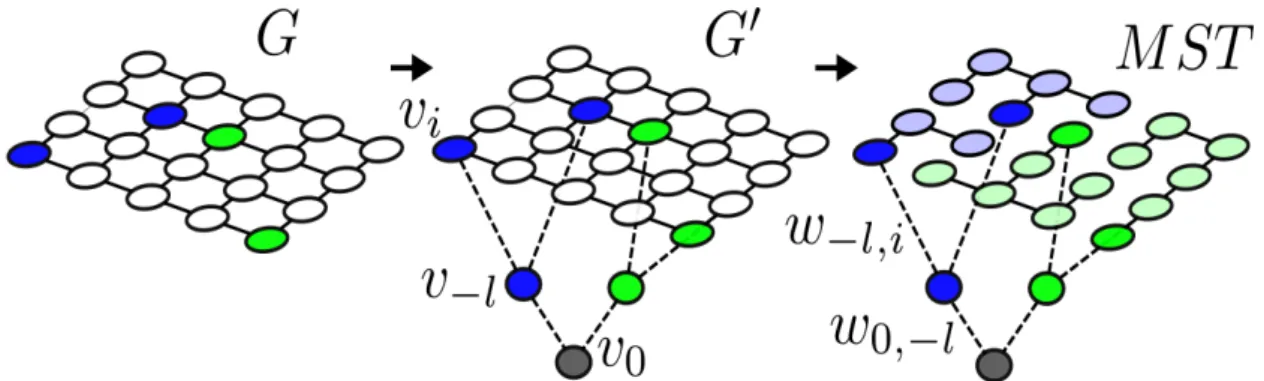
Figure 1.2: Seeded image segmentation using minimum spanning trees. The image nodes which the user has seeded (blue, green) are connected to virtual seed nodes v−l which in turn are connected to a virtual root nodev0. The associated edge weights are set to0which ensures that
the edges belong to the minimum spanning tree of the augmented graphG0. The final label of an image node depends on the subtree to which the node is assigned in the resulting minimum spanning tree.
1.5 Watershed cuts and minimum spanning trees
It is well known [35] that the watershed cut is equivalent to a minimum spanning forest calcu-lation or a minimum spanning tree computation on an augmented graph. Such a suitably aug-mented graphG0 = (V0, E0)can be constructed by adding a supernodev0 connected to newly
added seed nodesv−l, l∈Lfor each class type that are connected tov0with zero weight edges.
All labeled nodes (i.e. all supervoxels holding a user seed) are also connected to these seed nodes with zero-weight edges. These zero weight edges guarantee that the edges are part of a MST. Once the MST with root nodev0has been constructed, subtrees originating from seed nodesv−l form segments of the final segmentation. This graph construction is shown in Figure 1.2. The subtrees and the segmentation of the seeded watershed cut are defined as follows:
Definition 1.5.1 (SubtreeTi) LetT be a spanning tree ofGwith root node v0. The subtree
Ti = (Vi, Ei)is defined as the set of nodesViand edges Eiwhich inT can only be reached from the root node by a path containingvi.
Definition 1.5.2 (Segmentationx) LetT be a spanning tree ofGwith root nodev0. The label
assignment of all nodes is called the segmentationx withxi = lif node vi is element of the subtreeT−lof seed nodev
−l. Thus, all nodesiwith labelxi=land the edges connecting them form the subtreeT−lofT with root nodev−l.
Why is a segmentation based on a minimum spanning tree computation called a watershed cut? Assume we are given an image where the pixel valuesh(i)of pixel i correspond to the height of a topographic surface. Applying the classical watershed algorithm would start by flooding this surface starting from the user given seeds until the water from different basins meets at so called watershed lines. For the MST based algorithm, we construct a pixel grid graph and associated
with each edge(i, j) a weightwij = h(i) +h(j)which encodes the average height between the two pixels. When computing the MST with Prim’s algorithm starting from the root node
v0we always follow the smallest edge weight first and attach the node which is incident to this
smallest edge weight to the current tree. The subtreesT−l grow in this fashion until they meet and all nodes have been assigned to one of the subtrees. Since this procedure is very similar to the flooding based classical node weighted watershed the name watershed cut coined in [35] is suitable.
1.6 Watershed edge weights
We have presented the underlying principle of the watershed algorithm: flooding a topographic surface from local minima or user given seeds. However, given an image and a segmentation task it is unclear what this topographic surface should be, or, in the context of the watershed cut: what are the best edge weights for the segmentation task. It is clear that the edge weights which indicate boundaries should be high where a desired segmentation boundary is located and should be low where the object or segment of interest is homogeneous. Thus, depending on the segmentation task, edge weights can be constructed for example from the gradient of the image which is suitable to detect step like boundary, i.e. transitions from one homogeneous color to another homogeneous color. Another useful boundary indicator is the largest eigenvalue of the Hessian matrix which is suitable for image boundaries that are represented by a thin dark or bright line.
1.7 Decision trees
Despite the hand-crafted edge weights which were presented in the previous Section 1.6, edge weights can also be learned as a combination of different boundary indicators from user an-notations. We will consider this boundary learning problem in Chapter 4 and Chapter 5. The boundary or edge-weight learning can be posed as a supervised learning problem where a clas-sifier is trained from positive (boundary) and negative (no boundary) examples. Each examplei
consists of aDdimensional feature vectorxi ∈ RD and an associated class labelyi ∈ {0,1}, whereyi = 1would correspond to a positive example andyi = 0would correspond to a nega-tive example. In a supervised machine learning setting many such examples are used to train a decision function that maps unseen query vectorsx∈RDto either the positive or negative class. The basis for many supervised machine learning algorithms are decision trees. One of the best known works on decision trees is the book Classification and regression trees by Breiman et al. [20]. The authors describe the basics of decision trees and their application to classification and regression tasks. A decision tree is a collection of nodes an edges organized in a hierarchical fashion as a binary tree with a dedicated root node. Nodes are divided into inner nodes and leaf nodes. The leaf nodes contain a decision making predictor such as a class label or a regression value. The inner nodesicontain binary test functionsh(x, θi)whose output can be either true
1.7 Decision trees
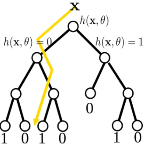
Figure 1.3: Decision tree illustration. Starting at the root node a test functionh(x, θ)is applied to a data samplex. Depending on wether the test function evaluates true (1) or false (0) the data sample is passed on to the right or left child of the current node. This process stops once the data sample reaches a leaf node and the corresponding class label stored at that node is returned.
or false. The output of the test function depends on the parametersθi associated with the inner nodeiand the feature values of the tested data samplex ∈Rd. Often the binary test function
h(x, θi)is a simple threshold test for a specific feature, i.e. it tests whether the feature valuexf of a data samplexfor featuref is above or below a certain threshold. At prediction time, a data samplexis passed down the tree until it reaches a leaf node. The path to the leaf node is given by the results of the binary tests which are applied at the inner nodes. Starting at the root node a binary test function is applied to the data sample. If the outcome is true the sample is passed to the left child node, if the outcome is false the sample is passed to the right child node. This process is repeated recursively until the data sample reaches a leaf node and the class label or regression value stored at that leaf node is returned.
During the training procedure of a decision tree the structure of the tree is determined as well as the split node parametersθi. We denote the set of training samples that belongs to a split nodeiasSi. An inner node or split node partitions this set of training samples into a left set
SiLand a right setSiR. These two sets are passed on to the left and right child node of the node under consideration. Thus,SiL = S2i+1 andSiR =S2i+2. The contents of the setSiLandSiR depend on the split parametersθi. During tree construction these split parametersθi of a node are optimized, such that an impurity criterion for the partitioned set is optimized with respect to their ground truth labels:
θ∗i = argminθiI(Si, SiL, SiR, θi)
whereI is a suitable purity criterion, like Gini impurity [19] or Entropy [37]. This partitioning of the data starts with a root node 0 and the set of all training samples S0 and is continued
1.8 Thesis overview
The watershed edge weights discussed in Section 1.6 are calculated from simple image filters. The image, and the filter response are subject to noise which may result in ambiguous or noisy edge weights. These erroneous edge weights in turn can lead to a wrong segmentation result. In Chapter 2 and Chapter 3 we study how uncertainty estimates for the segmentation can be constructed, that allow the user to find such potentially erroneous parts of the segmentation.
Furthermore, in many segmentation tasks the best boundary indicator is not just a simple im-age filter but a combination of many such filters on different scales. In Chapter 4 and Chapter 5 we investigate how such combined edge weights can be learned from sparse user annotations that do not need to be placed on the boundary itself. Instead we learn the edge weights from must-link and cannot link constraints between user given brush strokes, which is beneficial since these strokes are much easier to give.
One of those the boundary weight learning algorithms I propose is based on Multiple Instance Learning, a weakly supervised learning technique. This lead to research on Multiple Instance Learning algorithms itself. Thus, in Chapter 6 I propose a Multiple Instance Learning algorithm based on an optimized linear combination of decision trees.
Finally, in Chapter 7 a flow graph based computation library is presented which forms the backend of ilastik [110], the interactive learning and segmentation toolkit.
Chapter 2
Watershed uncertainty
2.1 Introduction
Interactive segmentation is a popular paradigm in image analysis because it combines the number-crunching capabilities of a computer with the high-level understanding of a human. When the segmentation result is immediately updated after each interaction, the user can readily spot er-rors and correct these by a (hopefully small) number of additional inputs. Unfortunately, this elegant scheme breaks down in 3D because errors no longer “pop out” to the user’s attention as they do in 2D – it is not possible to visualize complicated 3D segmentations in a way that makes user inspection and intervention as easy as in two dimensions. Most commonly, volume data is presented on a 2D screen by means of three orthogonal views, and the user has to scroll through several, and possibly many, layers in order to find or rule out segmentation errors.
We propose to solve this problem by guided interactive segmentation [43], akin to active learn-ing. Active learning (AL) [107] schemes aim at the steepest possible learning curve by querying for user input on locations which are regarded as most informative by a suitable selection cri-terion, so that user effort is focused on decisions with high impact. Accordingly, our algorithm not only proposes a segmentation based on the user’s inputs, but also estimates aconfidencein the segmentation result which will guide the user to locations where the uncertainty is highest. Good uncertainty criteria are especially challenging in our context because segmentation quality is a non-local property: A very small error (e.g. a single wrongly deleted boundary) can have catastrophic global consequences (such as an erroneous merge of two very large regions). Purely local error estimates as used in most existing AL work on interactive segmentation [9, 43, 117] are not sufficiently sensitive to these non-local effects.
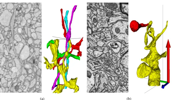
Our interactive segmentation framework is based on the watershed algorithm because it has a small computational footprint and is attractive for our target application: Microscopic images of neural tissue (see Fig. 2.1) are composed of very thin and elongated structures, which may pose a problem for the graph cut and random walk algorithms with their well-known shrinking bias.
(a) (b)
Figure 2.1: Raw data and ground truth. (a) Serial blockface electron microscopy (SBEM) image slice and 3D rendering of some neural processes from the image stack. (b) Focused ion beam electron microscopy (FIBSEM) image slice and two neural processes.
[80, 114] (see section 2.4.2). The goal of interactive segmentation is therefore to merge all super-voxels belonging to the same object. User labels are interpreted as seeds for either a foreground object or the background, and regions are defined according to a watershed cut initiated by these seeds [35].
Specifically we make the following contributions:
• We define and characterize a number of uncertainty criteria that can be used in the context of interactive segmentation with the watershed cut algorithm.
• We conduct extensive comparisons of the practical performance of these criteria in 3D neuro-imaging application examples.
• We demonstrate empirically that correct segmentations are achieved much faster when user attention is guided by our best active learning criteria.
2.2 Background and related work
2.2 Background and related work
Interactive segmentation algorithms must be able to take user input (“seeds”) into account and update results incrementally when new input arrives, and it must be sufficiently fast to ensure interactive response times. As explained in Chapter 1, some of the most important seeded seg-mentation methods can be unified in terms of thepower-watershedframework [32]. It defines a segmentation as a labeling of a graphG(V, E), where the optimal labeling xminimizes an energy function E(x,w) = X vi∈V w0p,ikxikq+wp1,ik1−xikq +X eij∈E wpijkxi−xjkq (2.1)
wherexi ∈Lis the label associated with nodevi ∈V,xis the vector of all label assignments, andwi,wij are node and edge weights, respectively. The first sum thus measures compatibility of the labeling with a given region model, whereas the second sum enforces smoothness of the solution. For different exponents, the power watershed specializes to the watershed cut algorithm (p → ∞,qfinite, [79], [35]), the random walker (pfinite,q = 2, [50]) and an Ising-type Markov random field amenable to graph-cut segmentation (pfinite,q = 1, [18]). A number of coarse-grained [29], pre-computed [51] or warm-started [62] strategies have been suggested to speed up the response to user input.
A significant simplification of the solution space is achieved by moving from a grid-graph defined on the original voxels to a coarser graph of supervoxels. The weighted graphs that reflect the supervoxel adjacency typically have a large total number of nodes, a small number of seeded nodes (the user scribbles), and are sparse (i.e. the number of edges is of the same order as the number of nodes). This is a favorable situation for power-watershed methods.
A number of user guidance schemes have already been proposed in the context of interactive segmentation for the random walker [43, 117] or graph cuts [9, 98]. These works use uncertainty cues based on the margin in the case of the random walk or min-marginal energies in the graph cut case [68], both of which capture mostly local information. In addition a perturbation based local uncertainty estimator for the graph-cut has recently been proposed in [98].
We propose several non-local uncertainty estimators for the watershed cut, and show that they perform better than a local alternative. Closest in spirit to our work are the stochastic topological watershed variants that have been proposed forunseeded segmentation [3, 92]. These authors consider a topological watershed from randomized seeds, while we randomize the edge weights instead.
2.3 Uncertainty measures for watershed cuts
We reviewed the notion of a watershed cut and its relation to a minimum spanning tree (MST) in Section 1.5 Now we will present two different types of uncertainty estimators. The first type presented in Section 2.3.2 is based on a minimal perturbation property and expresses how the obtained segmentation boundary depends on single edges in a graph. The second type of uncertainty estimators in Section 2.3.4 takes into account the uncertainty of the edge weights themselves. It measures how much the overall segmentation changes when sampling noisy edge weights.
2.3.1 Watershed cuts and minimum spanning trees
The interactive segmentation algorithm in this chapter is based on watershed cuts [79, 35]. It starts from a supervoxel graph which is computed by a standard flooding-type watershed algo-rithm [124] on a suitable boundary indicator, in our case the largest eigenvalue of the Hessian matrix which measures “ridgeness” and thus indicates cell membranes. The region adjacency graphG(V, E) of the supervoxels is equipped with edge weights that encode surface strength (in particular, the minimum value of the boundary indicator on the corresponding surface patch). User seeds provide hard assignments of some supervoxels to the background or one of the fore-ground regions.
As we explained in Section 1.5 the watershed cut is equivalent to a minimum spanning tree (MST) computation on a suitably augmented graphG0(V0, E0) that contains a supernode v0
connected to seed nodesv−l, l∈Lfor each class type that are connected tov0with zero weight
edges. All labeled nodes (i.e. all supervoxels holding a user seed) are also connected to these seed nodes with zero-weight edges, which are guaranteed to remain in the MST. Once the MST with root nodev0has been constructed, subtrees originating from seed nodesv−lform segments of the final segmentation. This graph construction is shown in Figure 1.2.
Since we are concerned with non-local uncertainty estimates that measure influences on the segmentation, we frequently rely on the definition of the edges connecting different segments: Definition 2.3.1 (Cut setC(T)) LetT be a spanning tree ofG. An edgee= (i, j)is element of the cut setC(T)if the verticesviandvjbelong to different subtreesT−l(Definition 1.5.1) so that the segmentation label (Definition 1.5.2)xi 6=xj.
In the following, we will introduce estimators arising from two different general principles. The first one analyzes the effect of single edge weight perturbations on the MST and the resulting segmentation, in a manner similar to [30]. The second estimator takes into account that the edge weights of the supervoxel graph are themselves subject to uncertainty, and measures how much the segmentation would change under perturbations of all weights.
As a baseline we compare our non-local estimators to alocal instabilitydefined by the mar-gin of the seeeded watershed cut: the marmar-gin is the difference between the maximum weight encountered on the lowest possible path from the winning seed type to the node under consider-ation minus the maximum weight on the lowest possible path from the second best seed type to
2.3 Uncertainty measures for watershed cuts
the same node.
2.3.2 Link instability via minimum perturbations
The first uncertainty measure we propose estimates the influence ofindividualedges on the final segmentation. In Lemma 2.3.4 we show that only the inclusion of edgesf ∈ C(T)from the current cut setC(T)(i.e.f /∈T) into the minimum spanning tree changes the resulting segmen-tation. We propose to measure the instability of all edgese ∈ T currently part of the MSTT
by calculating how often an edgeewould be removed from the MST when considering pertur-bations that would enforce the inclusion of an edgef ∈ C(T), /∈ T into the MST. i.e. weight perturbations that change the segmentation.
Algorithm 2.3.2.1 counts how often an edge which is part of the MST would be removed from the spanning tree considering all edge weight perturbations that change the segmentation (Definition 1.5.2) induced by the MST. The correctness of Algorithm 2.3.2.1 is shown in the
Algorithm 2.3.2.1Link Instability 1. Determine the cut setC(M ST).
2. Do a breadth first search starting from the root node of the MST and store at each noden
the edge with maximum weight encountered on the path from the root node to noden. 3. For each edge in the cut set: The exchange partner is the edge with maximum weight
stored in either end node of the cut edge. Increment the counter of that edge.
next section.
We note that the runtime of Algorithm 2.3.2.1 is linear in the number of edges of the graph and thus preserves the low computational overhead of the watershed cut. This follows from the fact that the computational complexity of the determination ofC(T), the breadth first search and the counter incrementation are all linear in the number of edges.
2.3.3 Correctness of algorithm 2.3.2.1
Our uncertainty measures estimate by how much the segmentation would change if the edges in the spanning tree were replaced, and how likely these replacements are. MST edge exchange has been investigated in [47], and we repeat a useful lemma and definition from there:
Definition 2.3.2 (e, f exchange) [47] LetTbe a spanning tree of graphG. Ae, f-exchange is a pair of edges,e, f wheree ∈T, f /∈T, andT \e∪f is a spanning tree. The weight of the exchangee, f isw(f)−w(e). The weight of treeT\e∪fis the weight of treeTplus the weight of the exchangee, f.
Lemma 2.3.3 [47] A spanning treeT has minimum weight if and only if noe, f-exchange has negative weight.
Since we are only interested in changes of the MST that cause changes in the induced segmen-tation, we analyze the sufficient and neccessary conditions that yield a different segmentation: Lemma 2.3.4 Ane, f-exchange resulting in a spanning treeT0=T\e∪f induces a watershed segmentation different fromT if and only iff ∈C(T).
Proof →: Lete, f be an exchange with edgee= (i, j) ∈ T and edgef = (k, l) ∈ C. Then, either node k or node l change their segmentation: before the exchange we obtain from the definition of the cut setC andf ∈ C: xk 6= xl, while after the exchange f ∈ T and thus
xk=xl.
←: Lete, f be an exchange with edgee= (i, j)∈ T and edgef = (k, l). Assumef /∈C. First considerf to connect two nodes in the same subtreeT−lofe, i.e.xi=xj =xk=xl=l. Thus ane, f exchange will not change the segmentation of any node. Now considerfto connect two nodes in a different subtreeT−l0 6=T−lthene, i.e.xi =xj =landxk=xl =l0, then the
e, fexchange will not produce a valid spanning tree: subtreeT−l0 contains a cycle, and subtree
Tlis partitioned into two components.
Relying on the notion of ane, f-exchange (Definition 2.3.2) we now proof the correctness of the edgelink instabilityAlgorithm:
Lemma 2.3.5 Algorithm 2.3.2.1 counts how often an edge in the minimum spanning tree is exchange partner in negativee, fexchanges resulting from all minimal single edge weight per-turbations that induce a different seeded watershed cut segmentation (Lemma 2.3.4).
Proof Item 1: When considering all segmentation changing perturbations involving a single edge, it suffices to consider thee, f-exchanges wheree ∈T andf ∈C(T). This follows from Lemma 2.3.4.
Item 2: When considering the minimal perturbations that move edge f ∈ C(T) into the minimum spanning tree via ane, f exchange, it suffices to consider the edges on the path from nodeior nodej to the root node v0, with edgef = (i, j): if the edgeewere not on a path
from nodeior nodejto the root nodev0, with edgef = (i, j), exchangingewithf would lead
to a cycle. The fact thatehas to be the edge of maximum weight on either path follows from the fact that we look for the minimum perturbation of edgef that would result in a negative
e, f-exchange.
From Item 1 and Item 2 follows that the algorithm is correct.
2.3.4 Uncertainty from stochastic graphs
Edge weights in the supervoxel graph are computed from local features. Since the raw data are noisy, the edge weights are necessarily noisy as well. We accomodate this uncertainty by moving from deterministic edge weights to stochastic ones, which are distributed according to a probability distribution reflecting the noise. In contrast to [3, 92] who obtain a stochastic watershed by random perturbations of the seed positions, we keep the seeds fixed and instead randomize the edge weights. In particular, we define the stochastic watershed cut by replacing
2.3 Uncertainty measures for watershed cuts
the original edge weightswij withw0ij ∼P Dij, whereP Dij is the weight distribution of edge
(i, j)that can be modeled by multiplicative noise, for example.
Consequently, the hard label assignmentxiof nodevi in the fixed-weight watershed cut will be replaced by the probability of a label assignmentpi(l), l ∈ L which depends on the edge weight distributionsP Dij ofalledges(i, j).
Ideally, we would like to compute these probabilities exactly, but the analysis in the following section shows that no efficient algorithm for this problem exists. This is why we study an approximation.
2.3.5 #P-hardness of stochastic watershed cut problem
In this section we will reduce the so calledl−mnetwork reliability problem [122, 17] which is #P-hard to a stochastic watershed cut problem. This shows that the stochastic watershed cut problem, i.e. to calculate the probability of the label assignmentxi for all nodes is also #P-hard. #P-hard is a complexity class introduced in [122]. While an NP-hard decision problem asks wether there is a solution to a given problem, the #P-hard problem is to count the number of solutions to a problem. This complexity class has been extended in [17] to allow the computation of a real number instead of the number of solutions to a problem. First we give a definition of thel−mnetwork reliability problem [17].
Definition 2.3.6 (l-m Network reliability problem) The two terminal network reliability prob-lem is defined on an undirected graphG(E, V)with edge weightswij ∼Bernoulli(pij)where
pij is the probability of the connection betweeniandj being active (whereas an inactive edge is equivalent to a non-existing edge). The two terminal network reliability problem is then to calculate the probability of the existence of a path between two nodeslandm.
IntuitionWe reduce thel−mnetwork reliability problem to a stochastic minimum spanning tree calculation by constructing a new graphG0 based onG. We add a new root vertex0toG0
and introduce two label vertices−1and−2. GraphG0 is constructed in such a way, that when a connection betweenlandmexists inGnodemis a child of vertex−1in a MST ofG0and a child of vertex−2in a MST ofG0if no connection exists in the original graphG.
The new graphG0(V0, E0)contains all edges and vertices of the original GraphG. In addition a root vertex0is introduced which is connected with zero edge weightw−1 0 = 0, w−2 0 = 0
to the new label vertices−1 and−2. Node−1is connected to nodel0 with zero edge weight
w−1l0 = 0. Thess zero edge weights ensure that the corresponding edges are included in any
MST ofG0.
In addition the newly introduced vertex−2is connected with weightw0−2i0 =α, α > 1to
all nodesi0 ∈V0 that are also present inG.
The edge weight distributions of the original edgeswi jofGare modeled as
w0i0j0 ∼ Bernoulli(1 − pij)∗β, β > α
Thus a random trial inGthat removes an edge(i, j)corresponds to an edge with weightw0i0j0 = β in G0. A random trial which leaves edge (i, j) intact in G induces an edge with weight
wi00j0 = 0inG0.
Lemma 2.3.7 The probability of the node m0 being a child of node −1 in the M ST(G0) is exactly the probability of a connection betweenmandlin the original graphG. Thus the two terminal network reliability problem can be reduced to a stochastic watershed cut.
Proof Consider a random draw of the edge weights. First we consider the case that the realized graph induced by the trial leavesl andm connected inG. It is easy to see that in this case
m0 must be a child of node−1in the MST of the corresponding realization of G0, since any spanning tree in which m0 is a child of vertex −2 must include an edge w−0 2i0 = α > 1,
while theconnectednessoflandmin the original graphGimplies by construction that a path
P(l0, m0)inG0 exists with edge weightsw0i0j0 = 0,∀(i0, j0) ∈ P(l0, m0). Thus any MST inG0
with root node 0will have node m0 andl0 in a subtree of node−1(which is by construction connected with zero edge weight tol0).
Secondly we consider the case that the realized graph induced by the trial leavesl andm
disconnected. It is also easy to see that in this casem0 must be a child of node−2in any MST of the corresponding realization ofG0, since any spanning tree connectingm0to node−1must include an edgew0i0j0 = β > αsince thedisconnectednessinGimplies that anyP(l0, m0) in G0 includes at least on edge of such weight (by construction of the edge weights inG0 which assigns weightw0i0j0 =βwhen the bernoulli trial in the original graphGremoves edge(i0, j0)).
Thus any minimum spanning tree connects nodem0 to node−2 since this incurs the cheaper maximum cost ofw−0 2m0 =α < β.
We showed that any random trial that leaveslandmconnected inGimplies thatm0is a child of node−1in theM ST(G0), while any random trial that disconnectslandminGimplies that
m0is a child of−2in theM ST(G0).
Since the final probability is defined by the outcome of all possible trials and the outcomes are linked in the described way it has been shown that thel−mterminal network reliability can be answered by calculating the probability form0 being a child of a newly introduced node−1
in aM ST of a newly constructed GraphG0. This is a stochastic watershed cut problem.
Sampling scheme
Since computing the exact label distribution is infeasible, we propose to sampletmaxcomplete graphsGt, t∈ {1, .., tmax}from the space of feasible graphs by sampling their edge weightswijt from the independent probability distributionsP Dij.
For each randomly drawn graph Gt, the seeded watershed cut is computed by calculat-ing the minimum spanncalculat-ing tree and assigncalculat-ing the node labels xti = l according to Defini-tion 1.5.2. After all repetiDefini-tions, the probability of node vi carrying label l can be estimated as pi(l) = tmax1 Pttmax0=1δ(xt
0
i, l). The final segmentation after tmax repetitions is defined as
xi = argmax l
pi(l), i.e.xiis assigned in a winner-take-all fashion to the labellto which nodei was most often assigned during the trials.
2.3 Uncertainty measures for watershed cuts
sampled graphs and the individual minimum spanning tree computations can be executed in parallel.
Stochastic uncertainty estimators
Uncertainty estimators based on the stochastic watershed cut can be defined in various ways, a natural one being the probability margin between the winning labelxi =land the one with the next highest class count, i.e.mi=pi(l)−pi(z0)wherez0 = argmax
l06=l cli0.
However, this is only a local estimator of uncertainty, whereas critical edges should be charac-terized by theirnon-localeffects. By combining the link instability according to Algorithm 2.3.2.1 with stochastic watershed cuts by accumulating the link instability of the edges over alltmax
tri-als, a measure incorporating the influence of a single edge on theglobalsegmentation can be obtained. This estimator is calledstochastic link instability.
Algorithm 2.3.5.1Stochastic segmentation instability • Dotmaxtimes
1. Construct graphGtby samplingwijt fromP Dij.
2. ConstructM ST(Gt)with root node0, and store the segmentationxt. 3. Calculate and store the size of the subtreehti =|Ti|of each nodei. • Calculatepi(l) = tmax1 Pttmax0=1δ(xt
0
i, l)
• Calculate the final segmentation from the winning label for each node: xi =
argmax
l
pi(l).
• Calculate the cut setCinduced byx.
• Aggregate for each nodeiwith edge(i, j)∈C, i.e. for all nodesitouching the segmen-tation border, the size of the subtreeshtiover all trials where the labelxtidiffered from the winning labelxi:Hi=Pt0:xt
i6=xih t0 i
Finally we propose another non-local alternative. Algorithm 2.3.5.1 takes advantage of an important property of the randomization of edge weights: the changing segmentation boundary (cut setC(Tt)) that results from each trial t of the stochastic watershed cut. This effect can be incorporated into an uncertainty estimator which attributes the magnitude of the aggregated segmentation boundary movement throughout the trials to individual edges.
The intuition behind thestochastic segmentation instabilitymeasureHi is that very unstable segmentation boundaries indicate ambiguity in the data and need user verification. The definition ofHi (Algorithm 2.3.5.1) ensures that nodes receive high uncertainty when their label differs
(a) (b) (c) (d) (e)
(f) (g) (h) (i) (j)
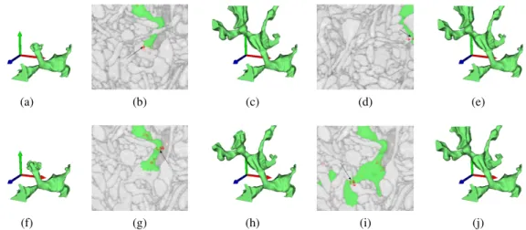
Figure 2.2: User guidance example for two of the proposed estimators. The top row displays the stochastic watershed using the stochastic segmentation instabiltiy estimator (Algorithm 2.3.5.1) , the bottom row the stochastic link instability estimator (Section 2.3.5). Displayed from left to right are the initial segmentation and two refinements based on seeding at the position of highest uncertainty (uncertainty is indicated by red color, the position of highest uncertainty by an arrow).
frequently from the winning label, or the affected subtrees are large. Nodes of highest criticality exhibit both problems.
2.4 Evaluation
2.4.1 Robot user
To evaluate the proposed uncertainty estimators objectively, we have designed an interactive segmentation robot [94]. The automaton tries to segment all neural processes in the data using two different seeding strategies. In theground truth strategythe robot places two initial seeds, one inside the object of interest, one outside and then loops until convergence:
1. Calculate the set differences between ground truth and current segmentation.
2. Place a correcting single voxel seed in the center (maximum of the Euclidean distance transform) of the largest false positive or false negative region.
3. Re-run the segmentation algorithm with the new set of seeds.
Note that this segmentation robot requires knowledge of the complete three-dimensional ground truth for each iteration. This is clearly unrealistic, because if this knowledge were so readily available, then interactive segmentation would not be required in the first place.
2.4 Evaluation
Theuncertainty query strategy, on the other hand, does not require full knowledge of the entire ground truth at each step. The robot begins by placing two initial seeds, one inside the object of interest, and one outside. It then loops until convergence:
1. Query the segmentation algorithm for the most uncertain region, using one of the confi-dence measures defined in Section 2.3.
2. Query the ground truth for the true label at the corresponding position. 3. Place a suitable seed at that position and re-run the segmentation algorithm.
2.4.2 Experiments
To evaluate the proposed uncertainty estimators for the seeded watershed cut we compare the estimators on a 3D segmentation problem from the neurosciences in a user guided segmentation setting. The nearly isotropic and densely annotated ground truth data is a subset of 400×
200×200voxels from a20003volume of neural tissue acquired with a serial blockface electron microscopy (SBEM [38], Figure 2.1) and a900×450×450densely annotated subset from a
20003volume acquired with focused ion beam electron microscopy (FIBSEM [67], Figure 2.1). The reconstruction of the neural processes in this tissue is a segmentation problem that exhibits many properties that make it suitable for the seeded watershed cut [114].
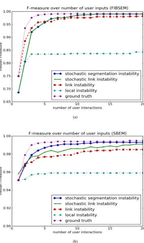
We have tested all proposed uncertainty estimators with the uncertainty query strategy of the robot user against theground truth strategy, which can be seen as an upper bound labeling strategy. During the segmentation process we recorded the resulting segmentation f-measure after each additional seed to compare the convergence rate of the robot for the different un-certainty estimators. Figure 2.3 shows the median across all neural processes in the respective ground truth. The parameters, namely the bias of the background seed (a background seed preference, [114]) and the amount of perturbation β in the case of the estimators based on thestochastic watershed cutwere determined by a grid search over a training set consisting of
10%of the neural processes. For simplicity, the edge weights for the trialstwere sampled as
wijt ∼ Unif(wij,(1.0 +β)∗wij). These edge weight distributions are simplistic, and even bet-ter results may be obtained when using more appropriate distributions. Figure 4.5 b displays the averaged standard deviation forpi(l)over100runs of the stochastic watershed cut with differ-ent trial countstmax. While the average standard deviation does not converge for the trial counts considered here, Figure 4.5 a indicates, that the number of randomly sampled graphs has vir-tually no effect on the predictive quality of the two proposed stochastic uncertainty estimators, already a trial size oftmax = 5can be used for successful user guidance. Thus our estimators incur only a small additional computational overhead compared to the standard watershed cut, which can be calculated in quasi linear time [28] (inverse ackerman complexity).
2.5 Conclusion
We have presented and evaluated several novel uncertainty estimators for the seeded watershed cut. The proposed estimators are based on a perturbation principle and stochastic edge weights, respectively. The proposed estimators were evaluated on a 3D biological neuroimaging applica-tion example that can profit from good uncertainty estimates and which exhibits many properties that make the seeded watershed cut a suitable algorithm. We showed that the proposed non-local uncertainty estimators yield a tremendous improvement in the number of user interactions com-pared to a simple local margin based approach which fails to query for more informative labels after the first few iterations. The proposed non-local estimators yield segmentation improve-ments that come close to an error correction strategy that relies on complete knowledge of the ground truth while incurring only an insignificant overhead compared to a standard watershed cut.
2.5 Conclusion
(a)
(b)
(a)
(b)
Figure 2.4: (a) Median F-measure over number of user interactions using 5 and 65 randomly sampled graphs. (b) Averaged standard deviation for pi(l) using 100 runs of the stochastic watershed over the number of randomly sampled Graphs along the x-axis.
Chapter 3
Enumerating the k best segmentation
changing spanning trees
3.1 Introduction
The most popular algorithms for interactive segmentation are Ising type Markov random fields (MRFs) [18], the random walker [50] and the seeded watershed [91]. Their smoothness terms penalize label changes with theL1,L2andL∞norms respectively [32]. However, in the process
of finding the single lowest energy solution to the graph partitioning problem a lot of information is lost and other modes of the solution space which may convey important aspects of the prob-lem are ignored. An enumeration of more than one low energy solution allows to obtain a more robust segmentation, and can help defining an uncertainty of the resulting segmentation which may be used in downstream processing. Thus, recent work on these algorithms has focused on finding the M lowest energy solutions [45, 95, 130], ideally subject to a diversity constraint [10]. These references solve the problem for Ising-type MRFs. However, systematic empirical studies [114] show that the seeded watershed outperforms MRFs in certain datasets and offers compu-tational advantages. The near linear runtime of a seeded watershed stems from its connection to the minimum spanning tree (MST) of the image graph [90, 35]. The present work presents the first viable algorithm that provides analogous M-best results for the seeded watershed cut. We build on the seminal work of Gabow [47] to enumerate only those spanning trees (ST) in an edge-weighted graph that lead to a change in the resulting segmentation. Furthermore we give a modification of Gabow’s algorithm that allows to enumerate the M-best diverse solutions simi-lar to [10], by enforcing a user specified distance between some of the generated segmentations. Such a diverse set of solutions can in turn be combined into a final segmentation [21].
3.2 Related work
The M-best solutions problem has been studied in the context of discrete graphical models [15] where it is known as the M-best MAP problem. Several types of algorithms have been pro-posed for the M-Best MAP problem: junction tree based exact algorithms [95, 106], dynamic programming based algorithms [105] and max marginal based algorithms [130]. An interesting extension of the M-best MAP problem was proposed and studied in [10]. Here, the authors give an algorithm to enumerate adiverse set of solutions. This is an attractive approach since the M-best solutions tend to be very similar to the MAP solution for a low M and thus important aspects of the solution space cannot be found. Generating such a set of diverse solutions was shown in [10] to remedy the problem of M-best solutions: when the initial M-best solutions are too close, important aspects of the solution space may only be found by enforcing a certain amount of diversity. The authors show that this diverse set of solutions which differ in a user specified amount from the MAP solution do not exhibit this problem.
The seeded watershed algorithm [91, 124] which we adapt enjoys great popularity in appli-cations where large amounts of data have to be processed, including medical and biological 3D image analysis [114], and where the shrinking bias typical of MRFs is detrimental.
We rely on the equivalence of the edge weighted seeded watershed and the minimum spanning tree (MST) algorithm [90, 35, 42] and draw on the seminal work of Gabow [47] who solved the k-smallest minimum spanning trees problem.
3.3 Image segmentation with minimum spanning trees
As explained in Chapter 1 we formulate the interactive image segmentation problem as a graph partitioning problem on the pixel neighborhood graphG(E, V). All neighboring pixelsv ∈V
are connected with edges (i, j) ∈ E. All edges have an associated edge weight wij ∈ R which expresses the dissimilarity between the neighboring pixels. The edge weightswij can be computed for example from the color gradient or another suitable boundary indicator. It is well known [90, 35] that the seeded watershed cut on a graphGis equivalent to a minimum spanning tree computation on a suitably augmented graphG0(V0, E0)that contains a supernode
v0 connected to seed nodes v−l for each label classl ∈ L. These seed nodes are connected to the root nodev0 with zero weight edges. All labeled nodes (i.e. all supervoxels holding a
user seed) are also connected to these seed nodes with zero-weight edges wi,−l = 0, which are guaranteed to remain in the MST. Once the MST with root nodev0 has been constructed,
subtrees originating from seed nodesv−l form segments of the final segmentation. This graph construction is illustrated in Figure 1.2.
3.4 Gabow’s algorithm for the k smallest spanning trees
3.4 Gabow’s algorithm for the k smallest spanning trees
The MST segmentation algorithm outlined in the previous section finds a single smallest span-ning tree of the augmented graph. In the next section, we will propose to generalize the algo-rithm by Gabow [47] to enumerate spanning trees that result indifferentsegmentations. To lay the foundation for our extension, we start with a description of Gabow’s original algorithm.
Gabow’s algorithm starts with a minimum spanning tree for the graph generated by e.g. Kruskal’s algorithm. This MST constitutes the first solution. The algorithm then enumerates different spanning trees in the order of increasing weight by swapping out an edge ebelonging to the current spanning tree, and replacing it by another edgef which is currently not in the tree.
To obtain the smallest spanning tree under such a so-called e, f-exchange, it finds the pair
e, fthat gives the smallest weight increasew(f)−w(e).
The main idea of the algorithm is to maintain a set of branchings and two lists associated with each branch, called IN and OUT, which prevent the algorithm from enumerating a spanning tree twice. All edges contained in the IN list have to stay in the spanning tree and all edges contained in the OUT list cannot enter the spanning tree.
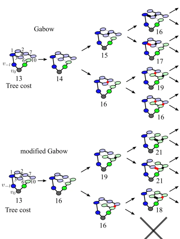
To enumerate all spanning trees in order, the algorithm finds the smallest weighte, f-exchange which is feasible according to the IN and OUT lists of the current state and branches on this exchange. Branching is done by considering two different cases: one branch is constructed by adding thef edge to the OUT list, the other branch is established by addingfto the IN list. Any further branching which is executed in the two cases inherits the respective IN and OUT lists from its parent state. Thus, any spanning tree constructed in the first branch excludes edgef and any spanning tree constructed in the second branch includes edgef. By visiting all branchings strictly in the order of increasing tree weight, the firstkminimum spanning trees are constructed in the correct order. This process is illustrated in Figure 3.1.
3.5 Enumerating changing segmentations
While Gabow’s algorithm finds the k smallest spanning trees of a given graph, it cannot be used to find the different modes of a segmentation: a grid graph has exponentially many spanning trees (1040for a 4-connected grid graph of size10×10, [119]). In typical images, exceedingly many spanning trees lead to the same segmentation. This effect is visible in the illustration of Gabow’s algorithm in Figure 3.1: while the algorithm always produces a new spanning tree, the associated segmentation does not necessarily change. This is especially true when there are large basins, or areas with low edge weights, as are typical for graphs constructed from natural images.
Thus, when generating thek smallest spanning trees, many if not all (when kis small) of the trees correspond to the same segmentation result. Luckily we can identify the sufficient and necessary condition that leads to a different segmentation result (compared to the previous state) in ane, f-exchange in Gabow’s algorithm.
Figure 3.1: Illustration of Gabow’s algorithm and our modification (best viewed in color). The algorithm of Gabow branches after each e, f-exchange into an upper case where the edge f
(indicated by thick black stroke) must stay in the tree and a lower case where the edgef (thick red stroke) must stay out of the tree. Our modified algorithm works in the same way, but only considers edgesf ∈ C(ST) which are part of the cut set for the current spanning tree. By definition, this induces a changed segmentation in each step. In contrast, in the original Gabow 28
3.5 Enumerating changing segmentations
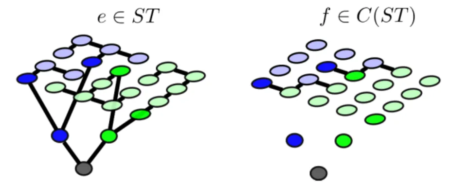
Figure 3.2: Illustration of cut edges. On the left, all edges of a spanning tree (ST) are shown in bold. In the middle all edges not belonging to the spanning tree a shown. The subset of the middle edges which belong to the seeded watershed cut – i.e. the edges which connect the different segments – are shown on the right. We modify Gabow’s algorithm by only considering these cut edges in anye, f-exchange. This enforces a changing segmentation between any two STs in the hierarchy of Figure 3.1, but does not guarantee that all resulting segmentations are unique.
In the case of a spanning tree segmentation, the assigned label (color) of a node depends on the subtree to which the node is connected in the spanning tree: the node is assigned the label of the virtual seed nodev−lof which it is a child in the spanning tree (see Figure 1.2). All edges in the spanning tree connect nodes of thesamecolor. An edge connecting two nodes ofdifferent color cannot be part of the spanning tree segmentation.
Now, if an e, f-exchange removes an edge e from the tree and replaces it with an edgef
that connects two nodes of the same color it is clear that the segmentation cannot change: the resulting spanning tree is merely a different way to express the same segmentation.
We now come to the core idea: to enforce a different segmentation, the edgef that is swapped in has to connect two nodes ofdifferentcolors. After swapping in the edgef, both nodes belong to the same subtree and thus one of the two nodes changes its color. The resulting segmentation is different.
We call these edgesf that connect nodes of different color in a ST segmentation “cut edges”
f ∈C(ST). See Figure 3.2 for an illustration.
At this point, we are able to modify Gabow’s algorithm to not only enumerate different span-ning trees in order of increasing weight, but to enumeratechangingsegmentations in the order of increasing weight.
A small change is sufficient to reach the desired behavior: by adding all edgesfwhich are not part of the cut set to a list OUTC={f :f /∈C(ST)}, Gabow’s algorithm can only consider edges f ∈ C(ST) for any e, f-exchange since all edges in the OUT and OUTC list are not eligible. Thus the segmentation of any spanning tree that is generated differs from the previous segmentation. The OUTC list is always updated once a new spanning tree has been generated
![Figure 1.1: Interactive segmentation illustration. The left picture shows a image from the BSD300 [85] segmentation database and a set of foreground and background seeds a user might give](https://thumb-us.123doks.com/thumbv2/123dok_us/10200892.2923053/14.892.147.767.177.388/figure-interactive-segmentation-illustration-segmentation-database-foreground-background.webp)
![Figure 3.3: Modified Gabow example. The top-left image shows an electron micropscopy image of cells in neural tissue [22] and user given seeds (red,green)](https://thumb-us.123doks.com/thumbv2/123dok_us/10200892.2923053/42.892.237.677.169.359/figure-modified-gabow-example-electron-micropscopy-neural-tissue.webp)