Some pages of this thesis
may
have been removed for copyright restrictions.
If you have discovered material in AURA which is unlawful e.g. breaches copyright, (either
yours or that of a third party) or any other law, including but not limited to those relating to
patent, trademark, confidentiality, data protection, obscenity, defamation, libel, then please
read our
Takedown Policy
and
contact the service
immediately
Pattern Integration in the Normal and Abnormal Human
Visual System
Alexander Scott Baldwin Doctor of Philosophy
Aston University March, 2013
c
Alexander Scott Baldwin, 2013
Alexander Scott Baldwin exerts his moral right to be identified as the author of this thesis.
This copy of the thesis has been supplied on condition that anyone who consults it is understood to recognise that its copyright rests with its author and that no quotation
from the thesis and no information derived from it may be published without proper acknowledgement.
Thesis Summary
Aston University
Pattern Integration in the Normal and Abnormal Human Visual System
Alexander Scott Baldwin
PhD candidate in Neurosciences Submitted: 2013
The processing conducted by the visual system requires the combination of signals that are detected at different locations in the visual field. The processes by which these signals are combined are explored here using psychophysical experiments and computer modelling. Most of the work presented in this thesis is concerned with the summation of contrast over space at detection threshold. Previous investigations of this sort have been confounded by the inho-mogeneity in contrast sensitivity across the visual field. Experiments performed in this thesis find that the decline in log contrast sensitivity with eccentricity is bilinear, with an initial steep fall-off followed by a shallower decline. This decline is scale-invariant for spatial frequencies of 0.7 to 4 c/deg. A detailed map of the inhomogeneity is developed, and applied to area sum-mation experiments both by incorporating it into models of the visual system and by using it to compensate stimuli in order to factor out the effects of the inhomogeneity.
The results of these area summation experiments show that the summation of contrast over area is spatially extensive (occurring over 33 stimulus carrier cycles), and that summation be-haviour is the same in the fovea, parafovea, and periphery. Summation occurs according to a fourth-root summation rule, consistent with a “noisy energy” model. This work is extended to investigate the visual deficit in amblyopia, finding that area summation is normal in amblyopic observers. Finally, the methods used to study the summation of threshold contrast over area are adapted to investigate the integration of coherent orientation signals in a texture. The re-sults of this study are described by a two-stage model, with a mandatory local combination stage followed by flexible global pooling of these local outputs. In each study, the results sug-gest a more extensive combination of signals in vision than has been previously understood. Keywords:psychophysics, spatial vision, pattern vision, contrast, area summation
Acknowledgements
I primarily wish to acknowledge the assistance and support I have received from my supervi-sor, Tim Meese. I would also like to thank the other members of the Sensory and Perceptual Systems research group at Aston University. I am particularly grateful to Mark Georgeson, Daniel Baker, Robert Summers and Stuart Wallis for their advice. Daniel Baker assisted with the experiment design for Chapters 4 and 6 of this thesis.
Conducting the research for this thesis involved visiting McGill Vision Research on two occa-sions (summers of 2011 and 2012). I would like to thank Robert Hess, Kathy Mullen, Jesse Husk, Pi-Chun Huang, and Simon Clavagnier for their hospitality and assistance. Robert Hess and Kathy Mullen provided lab space and equipment that I used to perform my experiments. Jesse Husk, Pi-Chun Huang, and Simon Clavagnier helped me recruit amblyopic observers for Chapter 8 of this thesis. Robert Hess and Jesse Husk assisted with the experiment design and observer recruitment for Chapter 9.
I am also grateful to all of the observers who participated in my experiments, and to my friends and family for their support over the past four years.
Publications
Some of the work published in this dissertation has previously been presented in poster form at scientific conferences:
AVA Spring Meeting 2010 (Liverpool Hope University). Baldwin, A. S., Meese, T. S., and Baker, D. H. (2010). Loss of contrast sensitivity at 4 c/deg depends on eccentricity and meridian but not grating orientation for the central 9 deg of the visual field.Perception39(8):1151. AVA Christmas Meeting 2010 (Descartes University). Baldwin, A. S., Meese, T. S., and Baker, D. H. (2011). Retinal inhomogeneity and the witch’s hat: contrast sensitivity declines as a bi-linear function of eccentricity in each direction.Perception40(1):112.
AVA Spring Meeting 2011 (Cardiff University). Baldwin, A. S., Meese, T. S., and Baker, D. H. (2012). Extensive physiological summation of contrast signals over area revealed by wit-ch’s hat compensation for retinal inhomogeneity.Perception41(3):366.
ECVP 2012 (Alghero, Sardinia). Baldwin, A. S., Meese, T. S., and Baker, D. H. (2012). A reeval-uation of area summation of contrast with compensation for retinal inhomogeneity.
Per-ception41 (ECVP Abstract Supplement):223.
AVA Christmas Meeting 2012 (UCL). Baldwin, A. S., Husk, J. S., Meese, T. S., and Hess, R. F. (2012). Pooling strategies for the integration of orientation signals depend on their spa-tial configuration.Perception41 p. 1512.
Additionally, the study in Chapter 4 has been published as a paper:
Baldwin, A. S., Meese, T. S., and Baker, D. H. (2012). The attenuation surface for contrast sen-sitivity has the form of a witch’s hat within the central visual field. Journal of Vision, 12(11): 23 pp. 1-17.
Contents
List of Figures 12 List of Tables 26 1 Introduction 29 1.1 This thesis . . . 30 2 Literature Review 31 2.1 Introduction . . . 312.2 Basic architecture of early vision . . . 31
2.2.1 The retina . . . 31
2.2.2 The brain . . . 32
2.2.3 Inhomogeneities . . . 32
2.3 Filters, channels and transducers in the visual system . . . 33
2.3.1 Spatial filtering . . . 33
2.3.2 Spatial frequency and orientation channels . . . 34
2.3.3 Nonlinear transduction . . . 34
2.3.4 Uncertainty . . . 35
2.4 Psychophysical theory . . . 35
2.4.1 Sensory thresholds . . . 35
2.4.2 High threshold theory . . . 37
2.4.3 Signal detection theory . . . 37
2.4.4 Low threshold theories . . . 38
2.5 The interpretation of area summation data . . . 38
2.5.1 Combining signals from several detectors . . . 38
2.5.2 Linear summation . . . 39
2.5.3 Summation following nonlinear transduction . . . 40
2.5.4 Ideal summation using templates . . . 40
2.5.5 Probability summation under HTT . . . 41
2.5.6 Probability summation under SDT . . . 41
2.5.7 Combination models . . . 41
2.6 Summation of contrast to threshold . . . 42
2.6.2 Previous results from luminance-defined stimuli . . . 42
2.6.3 Previous results from contrast-defined stimuli . . . 43
2.6.4 Conclusions from previous contrast detection threshold studies . . . 44
2.6.5 Area summation in contrast discrimination studies . . . 44
2.7 Signal combination over area in other domains . . . 45
2.7.1 Summation of motion . . . 45
2.7.2 Summation of orientation . . . 45
2.8 Amblyopia . . . 46
2.8.1 Aetiology . . . 46
2.8.2 Effects on performance in visual tasks . . . 46
2.9 Conclusion . . . 47 3 General methods 48 3.1 Introduction . . . 48 3.2 Measures . . . 48 3.2.1 Visual angle . . . 48 3.2.2 Spatial frequency . . . 48 3.2.3 Orientation . . . 48 3.2.4 Contrast . . . 49 3.2.5 Size . . . 49 3.2.6 Signal-to-noise ratio . . . 50 3.2.7 Root-mean-square error . . . 50 3.3 Equipment . . . 50 3.3.1 CRT monitors . . . 50 3.3.2 Stimulus presentation . . . 50 3.3.3 Software . . . 51 3.4 Stimuli . . . 51 3.4.1 Gratings . . . 51 3.4.2 Raised-cosine envelopes . . . 52 3.4.3 Swiss cheeses . . . 54 3.4.4 Gabor patches . . . 55 3.4.5 Log-Gabor patches . . . 57 3.4.6 Battenberg patterns . . . 57 3.5 Procedures . . . 59 3.5.1 Two-interval forced-choice . . . 59 3.5.2 Single-interval identification . . . 59 3.5.3 Staircase methods . . . 59 3.6 Psychometric functions . . . 60
3.6.1 The psychometric function for detection . . . 60
3.6.2 The psychometric function for identification . . . 62
3.6.4 Palamedes . . . 62
3.7 Model fits . . . 62
3.7.1 Fitting models to data . . . 62
3.7.2 The downhill simplex method . . . 63
4 The visual field inhomogeneity in contrast sensitivity 64 4.1 Motivation and summary . . . 64
4.2 Introduction . . . 64
4.2.1 The visual field inhomogeneity in contrast sensitivity . . . 64
4.2.2 Effects of stimulus orientation . . . 65
4.2.3 This study . . . 67 4.3 Methods . . . 67 4.3.1 Equipment . . . 67 4.3.2 Stimuli . . . 68 4.3.3 Observers . . . 68 4.3.4 Procedures . . . 68
4.4 Results from Experiment 1 . . . 70
4.4.1 Contrast sensitivity across the central visual field . . . 70
4.4.2 Absolute orientation effects . . . 71
4.4.3 Relative orientation effects . . . 72
4.4.4 Results for vertical stimuli . . . 72
4.5 Results from Experiment 2 . . . 73
4.5.1 Finely-spaced mapping of contrast sensitivity . . . 73
4.6 Results from Experiment 3 . . . 75
4.6.1 Effects of spatial frequency . . . 75
4.7 Modelling . . . 75
4.7.1 Bilinear model equations . . . 75
4.7.2 Bilinear model comparison . . . 77
4.7.3 Determining the number of necessary model parameters . . . 79
4.7.4 Radial interpolation . . . 80
4.7.5 Scale invariance . . . 82
4.7.6 Comparison with physiology . . . 83
4.8 Further experiments in the periphery . . . 86
4.8.1 The sensitivity decline from 18 to 62 cycles . . . 86
4.8.2 Relative orientation effects appear on the horizontal meridian . . . 87
4.9 Discussion . . . 88
4.9.1 Bilinearity . . . 88
4.9.2 Scale invariance . . . 89
4.9.3 Orientation effects . . . 89
4.9.4 Meridional anisotropies and the attenuation surface . . . 89
5 Summation modelling 93
5.1 Introduction . . . 93
5.1.1 Analytic and stochastic models of area summation . . . 93
5.1.2 Fitting summation models to data . . . 93
5.2 Model stages . . . 94
5.2.1 Stimulus attenuated according to contrast sensitivity inhomogeneity . . 94
5.2.2 Spatial filtering by log-Gabor patches . . . 94
5.2.3 Rectification and nonlinear transduction of filter outputs . . . 96
5.2.4 Pixelwise additive Gaussian noise . . . 96
5.2.5 Template matching . . . 97
5.2.6 Spatial summation and calculation of the detection threshold . . . 98
5.3 Analytic predictions for models involving linear summation . . . 99
5.3.1 Building the summation models . . . 99
5.3.2 Linear summation model . . . 99
5.3.3 Nonlinear and quadratic summation models . . . 100
5.3.4 Template and ideal summation models . . . 101
5.3.5 Combination and noisy energy models . . . 103
5.4 Analytic approximations . . . 104
5.4.1 Models without linear summation stages . . . 104
5.4.2 HTT probability summation model . . . 105
5.4.3 SDT probability summation model . . . 106
5.5 Conclusions . . . 106
5.5.1 Summary of model predictions . . . 106
6 Area summation with witch hat compensation 108 6.1 Motivation and summary . . . 108
6.2 Introduction . . . 108
6.2.1 Area summation of low-contrast gratings to threshold . . . 108
6.2.2 This study . . . 109 6.3 Methods . . . 110 6.3.1 Equipment . . . 110 6.3.2 Stimuli . . . 111 6.3.3 Observers . . . 111 6.3.4 Procedures . . . 111 6.4 Results . . . 113 6.4.1 Gratings . . . 113 6.4.2 Swiss cheese . . . 114
6.4.3 Psychometric function slopes . . . 115
6.5 Modelling . . . 115
6.5.1 Analytic models of area summation . . . 115
6.5.3 Swiss cheese . . . 119
6.5.4 Interleaved designs and the matched template . . . 121
6.6 Discussion . . . 121
6.6.1 The integration of contrast over space is extensive . . . 121
6.6.2 Individual differences for the extent of area summation . . . 122
7 Area summation across the visual field 123 7.1 Motivation and summary . . . 123
7.2 Introduction . . . 123
7.2.1 Spatial summation along strips of grating . . . 123
7.2.2 Summation in the fovea and the periphery . . . 126
7.2.3 This study . . . 127 7.3 Methods . . . 129 7.3.1 Equipment . . . 129 7.3.2 Stimuli . . . 129 7.3.3 Observers . . . 130 7.3.4 Procedures . . . 130 7.4 Results . . . 132
7.4.1 Foveal and parafoveal tiger tail summation . . . 132
7.4.2 Peripheral tiger tail summation . . . 133
7.5 Modelling . . . 134
7.5.1 Model fitting . . . 134
7.5.2 Comparing the model predictions to the data . . . 136
7.5.3 Individual differences . . . 138
7.5.4 The stochastic max-across-templates model . . . 140
7.6 Discussion . . . 141
7.6.1 Summation behaviour is the same across the visual field . . . 141
7.6.2 Receptive field elongation and template effects . . . 142
8 Battenberg summation in amblyopes 143 8.1 Motivation and summary . . . 143
8.2 Introduction . . . 143
8.2.1 Battenberg summation in the normal visual system . . . 143
8.2.2 The neural deficit in amblyopia . . . 144
8.2.3 Area summation in the amblyopic visual system . . . 145
8.2.4 This study . . . 145 8.3 Methods . . . 146 8.3.1 Equipment . . . 146 8.3.2 Stimuli . . . 146 8.3.3 Observers . . . 146 8.3.4 Procedures . . . 148
8.4 Modelling . . . 149
8.4.1 Model architectures . . . 149
8.4.2 Model predictions . . . 151
8.4.3 Fitting the model predictions to the data . . . 151
8.5 Results . . . 152
8.5.1 Normal observer . . . 152
8.5.2 Amblyopic observers . . . 156
8.5.3 Artefacts . . . 163
8.6 Discussion . . . 166
8.6.1 Area summation in amblyopes appears to be normal . . . 166
8.6.2 Complications involved in the use of the Battenberg stimulus . . . 167
9 Summation of orientation signals 168 9.1 Motivation and summary . . . 168
9.2 Introduction . . . 168
9.2.1 Combining orientation signals over space . . . 168
9.2.2 Signal combination processes . . . 169
9.2.3 Pooling strategies and summation effects . . . 170
9.2.4 This study . . . 171 9.3 Methods . . . 171 9.3.1 Equipment . . . 171 9.3.2 Stimuli . . . 171 9.3.3 Observers . . . 173 9.3.4 Procedures . . . 174 9.3.5 Analysis . . . 175 9.4 Results . . . 175 9.4.1 Noise check . . . 175 9.4.2 Signal only . . . 177 9.5 Modelling . . . 178
9.5.1 Monte Carlo simulations . . . 178
9.5.2 Combination processes . . . 179
9.5.3 Vector averaging . . . 179
9.5.4 Filter maxing . . . 180
9.5.5 Pooling strategies . . . 181
9.5.6 Two-stage hybrid models . . . 182
9.5.7 Internal noise . . . 184
9.5.8 Effects of eccentricity . . . 184
9.6 Discussion . . . 185
9.6.1 Orientation integration is a noisy two-stage process . . . 185
9.6.2 The nature of the limiting internal noise . . . 186
10 Discussion 190
10.1 Conclusions from the work presented here . . . 190
10.1.1 The visual field inhomogeneity in log contrast sensitivity is bilinear . . . 190
10.1.2 Area summation is spatially extensive and occurs according to a single rule . . . 191
10.1.3 Summation of threshold contrast over area is normal in amblyopia . . . . 192
10.1.4 The summation of orientation signals is a noisy two-stage process . . . . 193
10.2 Future work . . . 194
10.2.1 Summation of contrast over space . . . 194
10.2.2 Integration of orientation signals . . . 194
10.2.3 Extending the orientation Battenberg work to the motion domain . . . . 195
10.3 Conclusion . . . 196
References 197 Appendices 209 A Birdsall’s theorem 210 A.1 Early noise and nonlinear transduction . . . 210
A.1.1 Single-channel systems . . . 210
A.1.2 Multi-channel systems . . . 211
A.1.3 Area summation with early noise . . . 212
B MATLABcode 214 B.1 Log-Gabors . . . 214
B.1.1 MATLABcode to produce log-Gabor patches . . . 214
B.1.2 loggabor.m . . . 214
B.2 The witch’s hat . . . 216
B.2.1 MATLABcode to produce a witch’s hat attenuation surface . . . 216
B.2.2 witchhat.m . . . 216
C Amblyope subjects 218 C.1 Table of amblyope subject information . . . 218
List of Figures
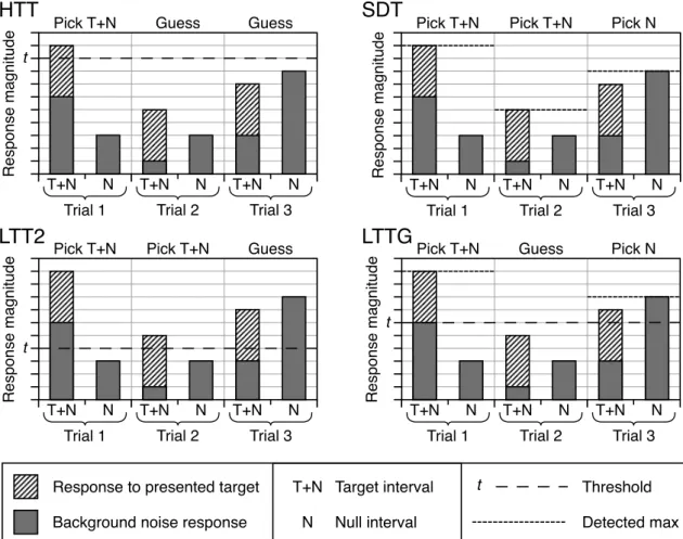
Figure 2.1 Graphs illustrating the behaviours of four detection theories: High Thresh-old Theory (HTT), Signal Detection Theory (SDT), Low ThreshThresh-old Theory with a Two State response (LTT2), and Low Threshold Theory with a Graduated re-sponse (LTTG). They show how an observer behaving according to each model would decide to respond in three example trials of a psychophysical task. The task is to determine which of two intervals contained a signal that is targeted to activate a single detector, added to a background of internal noise in that de-tector. The noise levels on each trial and interval have been chosen to illustrate the different behaviours of the four models. When operating under the HTT or LTT2 model, the systems make their choice purely based on whether an inter-val (either the T+N or N) has exceeded an internal threshold, the difference be-tween the two models being whether this threshold is set sufficiently high that it is never (or very rarely) activated by the internal noise alone. An observer operating according to the SDT model has access to a graduated response in each interval, so that the two values can be compared on each trial. The LTTG model also has access to this graduated response, but only for intervals where the internal (low) threshold has been surpassed. . . 36 Figure 2.2 The summation slopes predicted by five different summation models,
showing how detection threshold (in dB, see Section 3.2) declines as a function of stimulus area (expressed as20×log10(stimulus area)for ease of presenta-tion). The linear summation prediction has a slope of−1. The quadratic and ideal summation predictions both have a slope of−1
2. The probability and noisy
energy (ideal summation with a square-law transducer) predictions both have a slope of−1
Figure 3.1 Horizontal cross-sections (a-c) through the centres of example stimuli (d-f). Black lines in panels a) to c) show the stimulus luminance (varying from its minimum atLminto its maximum atLmax about the mean luminanceL0), the
dashed grey lines show the envelope that is being applied to the carrier grat-ing. Dashed white lines in panels d) to f) show where the cross section is taken. Panels a) and d) show a vertical sine-wave grating stimulus with wavelengthλ.
Panels b) and e) show this sine-wave grating windowed by a raised-cosine en-velope with a plateau width of 6λand a cosine section width of 12λ. Panels c)
and f) show that same windowed grating with “Swiss cheese” modulation. The modulator wavelength is 3.2λ, giving 1.6 cycles of grating per modulator “check”. 52
Figure 3.2 Panel c) shows a vertical Gabor stimulus with wavelengthλ, an
orienta-tion bandwidth of±25◦and a spatial frequency bandwidth of 1.6 octaves. Panel a) shows a cross-section through its horizontal centre (the dashed white line in panel c). The luminance profile of the stimulus (varying from its minimum at
Lminto its maximum atLmaxabout the mean luminanceL0) is plotted in black,
the envelope in dashed grey. Panels b) and d) show a log-Gabor stimulus with the same wavelength and bandwidths, and its cross-section. . . 55 Figure 3.3 Panels c) and d) show the Fourier transforms of the Gabor and log-Gabor
stimuli in panels c) and d) of Figure 3.2. The spatial frequency passbands of these stimuli at their preferred orientations (along the grey dashed line) are shown in panels a) and b). These are plotted on linear axes expressed in terms of
fs, which is the preferred spatial frequency of the Gabor and log-Gabor patches. 56
Figure 3.4 Horizontal cross-sections (a-c) through example “Battenberg” stimuli (d-f). Solid black lines in panels a) to c) show the stimulus luminance (varying from its minimum atLminto its maximum atLmaxabout the mean luminanceL0), the
dashed grey lines show the envelope that is being applied to the carrier grat-ing. Dashed white lines in panels d) to f) show where the cross section is taken. Panels a) and d) show a full vertical Battenberg array with wavelengthλ.
Pan-els b) and e) show the array modulated to give the “black check” (no contrast in centre) condition with two cycles per check. Panels c) and f) show the array modulated to give the “white check” (contrast in centre) condition. . . 58 Figure 3.5 The effects of the parameters of a Weibull function. Starting with the
original function (grey line) in panel a), the black dashed curve shows the effect of varyingα, and panel b) shows the effects of varyingβandγ. Panel c) shows
the effect of varyingλand a function whereγ =λ. Parameters for the curves
are shown above the panels. . . 61 Figure 4.1 Cartesian-separable log-Gabor stimuli generated in cosine-phase with
Figure 4.2 Diagram showing the four meridians tested in these experiments, and the eccentricities (in carrier cycles) along those meridians that were used in Ex-periment 1. “F” marks the fixation circle. “+ve” and “-ve” labels refer to the di-rection along the meridian that is plotted in the graphs below. . . 69 Figure 4.3 Contrast sensitivity data from Experiment 1 for observers ASB (left) and
DHB (right), normalised to the observer’s sensitivity at fixation. The separate plots show the sensitivity data for the detection of a 4 c/deg log-Gabor patch for each meridian, as indicated by the diagram in each plot. The four sets of symbols show data from the different stimulus orientations (as indicated in the legend). Eccentricity is expressed in stimulus carrier cycles, the visual angle of the range shown here is +4.5 degrees to -4.5 degrees along each meridian. Error bars in this figure (and in all subsequent figures) show±1 standard error where visible. Where they are not visible this is due to their being smaller than the symbol size. . . 70 Figure 4.4 Contrast sensitivity across the cardinal meridians for all four observers.
Vertical log-Gabor stimuli with a spatial frequency of 4 c/deg were used. The black dashed lines presented here for comparison are the gradients for the ver-tical (0.5 dB/cycle) and horizontal (0.33 dB/cycle) meridians reported by Pointer and Hess (1989). . . 73 Figure 4.5 Fine-positioning data from Experiment 2 (triangles), plotted with the
data from Experiment 1 (circles). The data presented here are averaged across the four observers (ASB, DHB, SAW and TSM), and the four panels are fitted simultaneously with the eight-parameter witch’s hat bilinear model (see Mod-elling section). Parameters for the model fit shown here are provided in Ta-ble 4.4. The dotted lines extrapolate the initial (m1) decline. . . 74
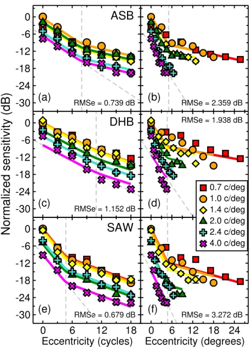
Figure 4.6 Contrast sensitivity decline data from Experiment 3 for six different spa-tial frequencies (indicated by their different symbols in the legend). Data are presented for the observers three ASB, DHB and SAW in separate rows. The two columns show the same contrast sensitivity data plotted against eccentric-ity expressed in stimulus carrier cycles on the left (panels a, c and e), and in de-grees of visual angle on the right (panels b, d and f). The solid curves are witch’s hat bilinear model fits to the data (see Modelling section). The parameters for these fits are provided in Table 4.6. The grey dashed lines show the positions of the fitted knee points (ν) and extrapolate the initial decline (with a negative
Figure 4.7 Comparison of the quality of the fits to the data provided by using the concave witch hat vs. the convex Samurai hat bilinear functions. Data are shown from the three main experiments and the two control experiments, with each hemi-meridian from each dataset being fitted independently by both models (each with four free parameters). The RMS errors from the two fits are plotted against each other in this scatter plot. For the purposes of presentation here, RMS errors larger than 3 dB were set to 3 dB (altering the position of a single data point so that it appears on the graph). The histogram shows the distribu-tion of the differences between the witch’s hat and Samurai hat model RMS er-rors, using the same colour code as the scatter plot. . . 78 Figure 4.8 A comparison of a direct fit to the data collected along diagonal
merid-ians in Experiment 1 against a prediction made by interpolating between the fitted horizontal and vertical meridians. The left and right plots show the data for ASB and DHB respectively. The direct fit is provided by fitting each diag-onal meridian individually with a four-parameter witch’s hat bilinear function, allowing the gradients (m1andm2) and knee point position (ν) to vary but fixing
the vertical offset (k2) across all four hemi-meridians (giving 13 free parameters
per plot). The interpolated fit was created by generating a surface using just the horizontal and vertical data, to then extract the radially interpolated diagonal values from that surface (no free parameters). For ASB the RMS errors for the direct and interpolated fits were 0.03 and 0.63 dB respectively. For DHB the RMS errors were 0.09 and 0.96 dB. The dotted grey lines are extrapolations of the gradient of the initial decline from the direct fit (m1). . . 81
Figure 4.9 A description of the decline in cone density (in thousands of cones/mm2)
with eccentricity, derived by fitting a 10thorder polynomial to the density data of Curcio, Sloan, Kalina, and Hendrickson (1990). Data were combined over the superior, inferior, nasal and temporal hemi-meridians. This one-dimensional function is radially interpolated to make the two-dimensional functiond, used
in the modelling here. . . 84 Figure 4.10 Relative contrast sensitivity predicted by the signal-to-noise ratios
de-rived from Equation 4.9 and the cone density data in Figure 4.9. Eccentricity is plotted in carrier cycles in the left column, and in degrees of visual angle in the right column. In the top row each curve is normalised to the SNR for the 0.7 c/deg patch at fixation. In the bottom row each curve is normalised to SNR for that curve at fixation. . . 85 Figure 4.11 Data from two observers (ASB and DHB) showing the decline in
con-trast sensitivity along the 45◦(upper-right diagonal) hemi-meridian to the four different patch orientations. The target spatial frequency was 4 c/deg. These data were collected at greater eccentricities than those tested in Experiment 1. The solid grey lines show linear fits to the most eccentric three data points (those at: 18, 40 and 62 cycles; equivalent to 4.5, 10, and 15.5 degrees). . . 86
Figure 4.12 Data from two observers (ASB and DHB) showing the contrast sensi-tivity to the four different patch orientations at an eccentricity of 62 cycles (15.5 degrees), as a function of hemi-meridian angle. The data for the 45◦
hemi-meridian are replotted from Figure 4.11. . . 87
Figure 4.13 A contour map of contrast sensitivity within the central 18 cycles of the visual field. The numbers labelling the contours indicate the amount of contrast attenuation (in dB). This map is based on a radial interpolation of the model fit to the average data in the bottom row of Table 4.4. . . 90
Figure 4.14 The same map of the contrast sensitivity inhomogeneity as that shown in Figure 4.13, displayed as a three dimensional surface. It is from the shape of this surface that the “witch’s hat” bilinear model draws its name. . . 91
Figure 5.1 Multiplication of the “Battenberg” stimulus in panel a) (see Section 3.4.6) by the witch’s hat attenuation surface in panel b) (see Section 4.9.4) gives the attenuated stimulus in panel c). The contrast of the image decreases from the centre outward at the same rate as the decline in contrast sensitivity in human vision. . . 94
Figure 5.2 The output of filtering the attenuated stimulus (Figure 5.1c) with a sine-phase log-Gabor (a) and a cosine-sine-phase log-Gabor (b). The simulated complex cell response calculated by taking the Pythagorean sum of the sine and cosine responses is shown in c). Inset in a) and b) are the sine-phase (Lsin) and cosine-phase (Lcos) log-Gabors used to perform the filtering. . . 95
Figure 5.3 The rectified output from filtering with a sin-phase log-Gabor patch (Fig-ure 5.2) is shown in panel a). The image in panel b) shows the effect of squaring the value at each pixel (representing the nonlinear transduction of filter outputs). 96 Figure 5.4 Noise is represented differently in the two types of model. In stochas-tic models (a) independent Gaussian noise is added to the pixel value at each location in the filtered stimulus image. In analytic models (b) the noise is repre-sented as a separate matrix containing the standard deviations of the noise for each pixel in the filtered stimulus. . . 97
Figure 5.5 Different template strategies are shown here, demonstrated using the stochastic model. Panel a) shows the noisy stimulus image with no template ap-plied. Panel b) shows the image multiplied by a template which is matched to the stimulus exactly (an “ideal” template). Panel c) shows the image multiplied by a template that is matched to the stimulus extent (without the “Battenberg” modulation). In both b) and c) the weighting of the templates declines with ec-centricity in proportion to the expected signal to noise ratio resulting from the attenuation surface. . . 97
Figure 5.6 Architecture of the linear summation model. . . 99
Figure 5.7 Architecture of the nonlinear and quadratic summation models. . . 100
Figure 5.9 Architecture of the combination and noisy energy models. . . 103 Figure 5.10 Architecture of the probability summation model under HTT. . . 105 Figure 5.11 Architecture of the probability summation model under SDT. . . 106 Figure 6.1 Example uncompensated and witch hat compensated grating (a-b), “black”
check “Swiss cheese” (c-d), and “white” check Swiss cheese (e-f) stimuli used in this study. Those shown are the largest of the stimuli used in this study (33 cycle diameter). . . 112 Figure 6.2 Contrast detection thresholds for the grating stimuli from ASB, DHB &
TSM, and the average of those data. Log-threshold (in dB) is plotted as a func-tion of the log of the squared stimulus diameter (the square of the diameter multiplied by a factor ofπ
4 gives the stimulus area, which would be a shift of -2.1
units on this axis). Panel a) shows the results for the flat stimuli, panel b) shows the results for stimuli that had been multiplied by the inverse of the witch hat attenuation surface. The solid, dashed, and dotted grey lines show slopes of
−1,−1
2, and− 1
4respectively. Error bars show±1 standard error here and in all
future graphs. . . 113 Figure 6.3 Contrast detection thresholds for the “Swiss cheese” stimuli from ASB,
DHB & TSM, and the average of those data. Average grating data are also re-plotted from Figure 6.2. Log-threshold (in dB) is re-plotted as a function of the log of the squared stimulus diameter (the scales of both axes are different from those in Figure 6.2). Panel a) shows the results for the flat stimuli, panel b) shows the results for stimuli that had been multiplied by the inverse of the witch hat attenuation surface. The solid, dashed, and dotted grey lines show slopes of
−1,−1
2, and− 1
4respectively. . . 114
Figure 6.4 Average grating data (replotted from Figure 6.2) fitted by the summation models described in Chapter 5. RMS errors and vertical offset parameters are provided in Table 6.2. Both rows show the same data. Panels a) and c) show the results for the flat stimuli, panels b) and d) show the results for stimuli that had been multiplied by the inverse of the witch hat attenuation surface. In panels a) and b), the data are fitted by the models which involve a linear transducer. These are the linear (L), template (two versions: matched template T and flat template FT), and probability summation (PS) models. In panels c) and d), the data are fitted by the models which feature a nonlinear transducer. These are the quadratic (Q) and noisy energy (two versions: matched template NE and flat template FTNE) models. . . 118
Figure 6.5 Average “Swiss cheese” data (replotted from Figure 6.3) plotted with area summation model predictions based on the fits shown in Figure 6.4. RMS errors are provided in Table 6.2. Results from grating stimuli are omitted from this figure to allow for a finer y-axis scale. All three rows show the same data. Panels a), c), and e) show the results for the flat stimuli. Panels b), d) and f) show the results for stimuli that had been multiplied by the inverse of the witch hat attenuation surface. Panels a) and b) show the probability summation (PS) model. Panels c) and d) show two versions of the noisy energy model with a template matched to the stimulus. Panels e) and f) show another two versions of the noisy energy model with a template matched to the stimulus extent. . . . 120 Figure 7.1 Results from previous studies that presented “tiger-tail” stimuli in the
fovea (these are listed in Table 7.1). Contrast detection thresholds were ex-tracted from the results presented in those publications and plotted (in dB re 1%) against the log stimulus area. Results are plotted separately for each ob-server (S1 - S2) in each study, and for whether the orientation of the grating stripes in the stimulus was horizontal or vertical. The solid, dashed, and dotted grey curves show slopes of−1,−1
2and− 1
4 respectively. . . 125
Figure 7.2 Results from Foley, Varadharajan, Koh, and Farias (2007), where “tiger-tail” stimuli were presented in the fovea (the details of this study are listed in Table 7.1). Contrast detection thresholds were extracted from the results pre-sented in this publication and plotted (in dB re 1%) against the log stimulus area. Results are plotted separately for each observer (S1 - S2) in the study. The solid, dashed, and dotted grey curves show slopes of−1,−1
2and− 1
4 respectively. . . . 126
Figure 7.3 Results from previous studies that presented “tiger-tail” stimuli in the periphery (these studies are listed in Table 7.1). Contrast detection thresholds were extracted from the results presented in those publications and plotted (in dB re 1%) against the log stimulus area. Results are plotted separately for each observer (S1 - S5) in each study, and for whether the orientation of the grating stripes in the stimulus was horizontal or vertical. The solid, dashed, and dotted grey curves show slopes of−1,−1
2and− 1
4 respectively. . . 128
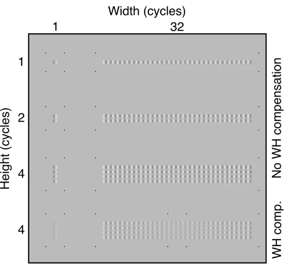
Figure 7.4 Examples of stimuli used in this study. The narrowest (1 cycle) and widest (32 cycles) examples of the non-compensated stimuli of each stimulus height (1, 2 and 4 cycles) are shown. Also shown are the quads of pixels shown around these stimuli that indicated the stimulus extent to the observer. Foveal witch hat compensated stimuli are shown for the the 1x4 and 32x4 stimulus condi-tions. These stimuli demonstrate the fixation paradigm used in the fovea, where fixation location was inferred from a quad of points (coincident with the stimu-lus extent quad for the 1x4 condition). . . 130
Figure 7.5 Diagram showing the stimulus locations tested in this study (not to scale). The circled "F" marking the fixation location was not present in the study. The fixation location was either inferred from the quad of points around the stim-ulus (in the fovea) or indicated by a 2 pixel square black dot (parafovea) or red LED (periphery). . . 131 Figure 7.6 Detection thresholds for “tiger-tail” stimuli presented in the fovea and
the parafovea (12 cycles eccentricity). Results are shown separately for the three observers. The top three panels (a-c) show thresholds for the condition with the non-compensated stimuli, the bottom three panels (d-f) show thresh-olds for the witch hat compensated stimuli. The data are fitted by predictions from the noisy energy (NE) model (see Section 7.5). In panels a) to c) the pre-dicted behaviour for the two stimulus locations is shown by the two vertically-offset curves plotted for each stimulus height. In panels d) to f) the model pre-dictions are identical, and so the two curves overlap. The solid, dashed, and dotted grey curves in this and all other figures show slopes of−1,−1
2 and− 1 4
respectively. . . 132 Figure 7.7 Contrast detection thresholds for “tiger-tail” stimuli presented in the
pe-riphery (centered at 42 cycles). The top two panels (a-b) show thresholds for the condition with the non-compensated stimuli, the bottom two panels (c-d) show thresholds for the witch hat compensated stimuli. The data are plotted with predictions made from the noisy energy model (NE) fit to the foveal and parafoveal data (dashed curves). Solid curves show direct model fits to the pe-ripheral data (see Section 7.5). . . 134 Figure 7.8 As Figure 7.6, but fitted with the flat template noisy energy model (FTNE).137 Figure 7.9 As Figure 7.7, but fitted with the flat template noisy energy model (FTNE).138 Figure 7.10 A modified version of the FTNE model fitted to the foveal and parafoveal
data for observer SAW (cf. Figure 7.8). For clarity, the data from the two loca-tions are shown in separate subplots (b-c) for the witch hat compensated stim-uli. The orientation bandwidth of the log-Gabor used in the filtering stage for the parafoveal stimuli was narrower (±14.7◦), elongating the simulated recep-tive field. The foveal and parafoveal data were fitted with separate vertical off-set parameters (10.25 dB for the foveal fit, 6.58 dB for the parafoveal fit). This model provides a superior fit to the data (RMSe = 0.71 dB). . . 139 Figure 7.11 Stochastic Monte-Carlo model predictions generated for the
max-across-templates noisy energy (MTNE) model. Average thresholds and the standard deviation of the threshold estimate (blue shaded region) were calculated from 10 repetitions of a simulated experiment (50 trials per point on every psycho-metric function in each repetition), using the witch hat attenuation surface from observer ASB. The MTNE model is plotted with the NE and FTNE models. . . 140
Figure 8.1 The “Battenberg” stimuli used in the experiments in this chapter. The full stimulus is shown, as well as the five different check sizes used in the ex-periments (check widths of 1, 2, 4, 6 and 8 elements). Each stimulus is shown in both the “black” and the “white” check phases. . . 147 Figure 8.2 “Battenberg” summation data for normal observers reproduced from
Meese (2010) and plotted with predictions from the probability summation model (PS), “max-across-templates” noisy energy model (MTNE), the “extent” noisy energy model (ENE), and the “flat extent” noisy energy model (FENE). The shaded area shows the standard deviation of the responses from the stochastic MTNE model. All model prediction curves, and the data from Meese (2010), were nor-malised so that the full (0) stimulus had a threshold of 0 dB. The spatial fre-quency used in Meese (2010) was 2.5 c/deg. . . 149 Figure 8.3 Detection thresholds for the “full” Battenberg stimuli for observer ASB
at three spatial frequencies (c1, c2, andc3). The labels a2 anda3 indicate the
spatial frequency of the artefacts introduced by the 1 by 1 check Battenberg modulation in the 4 c/deg and 8 c/deg stimuli respectively (see Section 8.5.3). . . 152 Figure 8.4 Detection thresholds from observer ASB for 2.5 c/deg “Battenberg”
stim-uli presented to the dominant (RE) and non-dominant (LE) eyes. The data are fitted by the prediction from the FENE model. . . 153 Figure 8.5 Detection thresholds replotted from Figure 8.4. The data are fitted by
the prediction from the PS model. . . 153 Figure 8.6 Detection thresholds from observer ASB for 4 c/deg “Battenberg”
stim-uli presented to the dominant (RE) eye. The data are fitted by the prediction from the FENE model. . . 154 Figure 8.7 Detection thresholds replotted from Figure 8.6. The data are fitted by
the prediction from the PS model. . . 154 Figure 8.8 Detection thresholds from observer ASB for 8 c/deg “Battenberg”
stim-uli presented to the dominant (RE) and non-dominant (LE) eyes. The data are fitted by the prediction from the FENE model. . . 155 Figure 8.9 Detection thresholds replotted from Figure 8.8. The data are fitted by
the prediction from the PS model. . . 155 Figure 8.10 Panel a) shows the average threshold differences between the two eyes
for each amblyope (S1 - S6) across the stimulus conditions tested here. Panel b) shows the difference in summation for each check condition, equivalent to the threshold difference between the two eyes normalised to that for the “full” (0) stimulus. . . 156 Figure 8.11 Detection thresholds from amblyopic observer S1 for 2.5 c/deg
“Batten-berg” stimuli presented to the fellow fixing (FFE) and amblyopic (AMB) eyes. The data are fitted by the prediction from the FENE model. . . 157 Figure 8.12 Detection thresholds replotted from Figure 8.11. The data are fitted by
Figure 8.13 Detection thresholds from amblyopic observer S2 for 2.5 c/deg “Batten-berg” stimuli presented to the fellow fixing (FFE) and amblyopic (AMB) eyes. The data are fitted by the prediction from the FENE model. . . 157 Figure 8.14 Detection thresholds replotted from Figure 8.13. The data are fitted by
the prediction from the PS model. . . 158 Figure 8.15 Detection thresholds from amblyopic observer S3 for 4 c/deg
“Batten-berg” stimuli presented to the fellow fixing (FFE) and amblyopic (AMB) eyes. The data are fitted by the prediction from the FENE model. . . 158 Figure 8.16 Detection thresholds replotted from Figure 8.15. The data are fitted by
the prediction from the PS model. . . 159 Figure 8.17 Detection thresholds from amblyopic observer S4 for 6 c/deg
“Batten-berg” stimuli presented to the fellow fixing (FFE) and amblyopic (AMB) eyes. The data are fitted by the prediction from the FENE model. . . 159 Figure 8.18 Detection thresholds from amblyopic observer S4 for 6 c/deg
“Batten-berg” stimuli presented to the fellow fixing (FFE) and amblyopic (AMB) eyes. These data are replotted from Figure 8.17 however the three conditions for which thresholds were unusually high in that figure are omitted here. The data are fitted by the prediction from the FENE model. . . 159 Figure 8.19 Detection thresholds replotted from Figure 8.18. The data are fitted by
the prediction from the PS model. . . 160 Figure 8.20 Detection thresholds from amblyopic observer S5 for 4 c/deg
“Batten-berg” stimuli presented to the fellow fixing (FFE) and amblyopic (AMB) eyes. The data are fitted by the prediction from the FENE model. . . 160 Figure 8.21 Detection thresholds replotted from Figure 8.20. The data are fitted by
the prediction from the PS model. . . 160 Figure 8.22 Detection thresholds from amblyopic observer S6 for 2.5 c/deg
“Batten-berg” stimuli presented to the fellow fixing (FFE) and amblyopic (AMB) eyes. The data are fitted by the prediction from the FENE model. . . 161 Figure 8.23 Detection thresholds replotted from Figure 8.22. The data are fitted by
the prediction from the PS model. . . 161 Figure 8.24 Example contrast sensitivity function (CSF) from the fellow fixing (FFE)
and amblyopic (AMB) eyes of an amblyope replotted from Hess, Campbell, and Greenhalgh (1978), Figure 7. The sold grey line labelledcmarks a possible
stim-ulus carrier frequency (2.5 c/deg) and the dashed lines labelleda1anda2show
the frequencies of the artefacts introduced below and above that spatial fre-quency by the 1 by 1 check Battenberg modulation. . . 163
Figure 8.25 Images of stimulus components (left column) and Fourier transforms of those images (right column). In the spatial domain, the full stimulus (bottom row) is the product of the carrier grating (top row) and the rectified orthogonal modulator grating (middle row). The modulator is generated at half the spatial frequency of the carrier (therefore it has the same periodicity after full-wave rectification). . . 164 Figure 8.26 Images of squarewave plaid modulator and 1 by 1 check “Battenberg”
stimulus (left column) and Fourier transforms of those images (right column). The Battenberg stimulus (bottom row) is the product of the full stimulus from Figure 8.25e and the squarewave plaid modulator (in the spatial domain). . . 165 Figure 8.27 Contrast detection thresholds for two amblyopic observers (S1 and S2)
at 1.8 and 2.5 c/deg. Data are shown for the fellow fixing (FFE) and amblyopic (AMB) eyes. . . 166 Figure 9.1 Demonstration of coherent texture. Panel a) shows an image of a
nat-ural scene. This was filtered by a pair of quadrature-phase vertical log-Gabor elements (inset), the complex response at each location was calculated as the Pythagorean sum of the sin and cosine responses. Pink locations in the image indicate where this response exceeded an arbitrary threshold. Panel b) shows the vertical energy in the image at the spatial scale at which the filtering in panel a) was conducted. The tree trunk on the left of the image, and the fences on each side of the bridge, are represented by clear regions of coherent vertical texture. . . 169 Figure 9.2 Example of the stimulus design used in these experiments. The stimuli
shown are 7 by 7 element arrays (smaller than the 29 by 29 arrays used in this study) with a 3 by 3 check size. The figure includes “white” and “black” check versions of the noise check and signal only stimuli, shown at 100% coherence. . 172 Figure 9.3 The numbers of potential signal and noise (always randomly-oriented)
elements in each stimulus. In the noise check stimuli (panel a) the total number of elements (841) remained constant. In the signal only stimuli (panel b) the checked stimuli contained approximately half as many elements as the full (0) stimulus. . . 173 Figure 9.4 Showing the method by which threshold coherence levels were
calcu-lated. Data from the two interleaved staircases (one for each signal orientation) were combined and fitted with a cumulative normal to give a single psychome-tric function. . . 174
Figure 9.5 Results from individual observers (see legend below) and the average re-sults across observers (right). Performance is expressed as the threshold pro-portion of coherent elements in the signal regions. Thresholds are expressed as multiples relative to that for the full (0) condition (these data are replotted in Figure 9.6). Results are shown for the noise check (a) and signal only (b) con-ditions. Error bars show±1 standard error here and in all other graphs. . . 175
Figure 9.6 The data from Figure 9.5 are replotted here as the threshold number of elements in the stimulus (panels a-b), the threshold percentage of signal ele-ments in the potential signal region (panels c-d), and the threshold percentage of signal elements in the entire stimulus (panels e-f). Other figures in this chap-ter use the representation of the threshold signal level shown in panels c) and d), with these “coherence thresholds” expressed as multiples relative to that of the full (0) stimulus. . . 176 Figure 9.7 Predictions for the noise check condition from models using the vector
averaging (a) and filter maxing (b) combination processes and a variety of dif-ferent pooling strategies. Each plot shows predictions for models that combine over all elements (SA), combine ideally (SI), and a two-stage hybrid model (HM) of mandatory local combination followed by ideal pooling (see Section 9.5.5). . . 178 Figure 9.8 Demonstration of the vector averaging combination process. The
orien-tation of each pooled element is input into the vector averaging formula (see Equation 9.1), from which the average orientation is then calculated. . . 179 Figure 9.9 The filter maxing combination process. The stimulus is filtered at the
two possible target orientations by log-Gabor patches matched to the signal elements. The magnitudes of the filter responses at each pooled location are then summed over the image and the responses from the two orientations are compared to pick the larger. . . 180 Figure 9.10 Showing the “sum all” (SA) and “sum ideally” (SI) pooling strategies. The
orange regions in the diagram show locations of potential signal elements, the blue regions show locations of noise or blank elements. The SA strategy com-bines information from all locations in the stimulus (signal and noise/blank), the SI strategy uses only information from the potential signal regions. The function f(X)represents either vector averaging or filter maxing depending on which combination process is being used. . . 181
Figure 9.11 Showing the pooling strategies used in the two-stage “hybrid models” (HM) and hybrid models with internal noise (HMN). In the HMN models the rep-resentation of the stimulus is perturbed by independent Gaussian noise added at each location (including blank regions). In the HM models no noise is added. Following this, mandatory local signal combination takes place over 3 by 3 re-gions to create a new matrix where each element represents the pooled infor-mation from a local region in the original image (at this stage behaving accord-ing to the SA strategy). This is then followed by flexible combination of infor-mation over that matrix, with the contribution from each element weighted ac-cording to its expected signal to noise ratio (at this stage behaving acac-cording to the SI strategy). . . 182 Figure 9.12 Coherence threshold data plotted with model predictions from the filter
maxing versions of the SA (a-b), SI (c-d), HM (e-f) and HMN (g-h) models. Each row shows the same averaged dataset replotted from Figure 9.5. The only fitted parameter was the size of the pooling regions in the HM and HMN models (3 by 3), which was performed by hand. RMS errors between the model predictions and data are shown in dB. . . 183 Figure 9.13 Coherence threshold data (replotted from Figure 9.5) plotted with model
predictions from the filter maxing version of the HMNI model. The mandatory pooling region was set to 3 by 3 elements, and the aperture beyond which ele-ments could not be pooled was set to 19 by 19 eleele-ments. These two parameters were fitted to the data by hand. RMS errors between the model predictions and data are shown in dB. . . 185 Figure 9.14 Diagram of the two-stage hybrid model with internal noise, using the
filter maxing combination process. This diagram shows how the “vertical” re-sponse is determined by filtering with a vertical filter element, mandatory local summation, and then global summation of the local outputs weighted by the ex-pected signal-to-noise ratio (w). The “horizontal” response would be calculated
in an identical manner, except with a horizontal filter element at the convolu-tion stage.Nearly,Nmid, andNlateshow three possible locations for the limiting
internal noise (discussed in the text). . . 187 Figure 10.1 Preliminary design for motion Battenberg stimuli (a). The phase of each
element will rotate to cause the perception of local motion in that element (tion vectors are shown by the black arrows). This can then give coherent mo-tion in elements that are in the signal regions of the checkerboard pattern (b, grey boxes indicate signal regions, background image omitted for clarity). This can also be done for stimuli where elements have different orientations to give a complex motion task (c). For this stimulus the rate of phase rotation in sig-nal elements will depend on their orientation, to give the impression of a single patterned object moving in one direction behind a grid of apertures. . . 195
Figure 10.2 Demonstrating the aperture problem for identifying the motion direc-tion of an object from its local modirec-tion vectors. The object in panel a) moves behind a screen with many apertures in panel b). The movement of the object’s edges seen within each aperture do not necessarily correspond to the direction of the motion of the object. For any single aperture these local motion vectors could correspond to several possible global motion directions (this is the aper-ture problem). Multiple motion vectors must be combined over space in order to calculate the true trajectory of the object. As each V1 neurone only receives information from a small part of the visual field these calculations must be per-formed by the visual system to determine the trajectory of any object. . . 195 Figure A.1 Psychometric functions generated from a stochastic Monte Carlo
simu-lation (5,000 iterations) of a detection task in a single-channel system (nc = 1)
featuring early Gaussian noise (µ = 0,σ = 1) followed by nonlinear transduc-tion with a range of different exponents (m). . . 210
Figure A.2 Psychometric functions generated from stochastic Monte Carlo simu-lations (5,000 iterations) of a detection task in systems with 100 and 10,000 channels featuring independent early Gaussian noise (µ = 0, σ = 1) in each channel followed by nonlinear transducers with different exponents (m). . . 212
Figure A.3 Summation behaviour in multi-channel systems with either “early” noise placedbeforenonlinear transduction, or “late” noise placedafternonlinear trans-duction. The early noise predictions are calculated from the mean of 20 stochas-tic Monte Carlo simulations (500 iterations each). The blue shaded area shows the standard deviation of the simulated data. Late noise predictions are derived using Equation 5.22. Models featured either 2, 100, or 10,000 channels, and a range of transducer exponents fromm = 1tom = 16. The summation ratio plotted is that between thresholds for stimuli presented to half of the channels or all of the channels in the system. The model featured a matched template, so the system monitored only relevant inputs (ignoring non-signal channels). . . 213
List of Tables
Table 4.1 Summary of stimulus and experiment details from previous studies that investigated the decline in contrast sensitivity with eccentricity. Where studies consisted of multiple experiments the details shown are for the experiments most similar to those conducted in this study. Abbreviations: H = Horizontal, V = Vertical and D = Diagonal. . . 66 Table 4.2 Log-contrast sensitivity decline gradient (in dB) for linear fits to
Experi-ment 1 data. Averages are given as the mean±1 standard error. . . 71
Table 4.3 Number of parameters, RMS error, and Akaike’s Information Criterion for five different versions of the witch’s hat bilinear model which were used to fit the combined data from Experiments 1 and 2 (data were averaged across the four observers). The variant in the bottom row is the preferred model (it has the lowest AIC score), its parameters are given in Table 4.4 and it is shown fitted to the data in Figure 4.5. . . 79 Table 4.4 Parameters obtained from fitting the preferred (eight-parameter) witch’s
hat bilinear model (see Table 4.3) to the combined data from Experiments 1 and 2. Different rows show the parameters given by fitting to each observer’s data individually, and to the average of the observers’ data. . . 80 Table 4.5 RMS errors for the 2x2x2 factorial model analysis. This covers each
possi-ble combination of the two methods of scaling the model parameters (i.e. whether they are fixed across spatial frequency in terms of carrier cycles or in terms of visual angle). Each model variant was fit to individual datasets from Experiment 3 for each observer (the models in the leftmost and rightmost columns of this table are shown in the left and right columns of Figure 4.6 respectively), and to data averaged across the three observers. The models were fit to the data from all spatial frequencies simultaneously in each case. For space reasons, the “dB/cycle” and “dB/degree” units in the row of the table defining the behaviour of them2parameter are abbreviated to “cy” and “deg” respectively. . . 82
Table 4.6 Parameters for the witch’s hat bilinear model fits to the data from Exper-iment 3 for each observer (plotted in the left column of Figure 4.6) and to the data averaged across the three observers. . . 83 Table 6.1 Stimulus diameters and the signal areas where the stimulus is above
Table 6.2 Models tested in this study, and the codes used in Figures 6.4 and 6.5. Information is provided about each model’s transduction and template stages, and whether signals are combined by a linear sum or a max operator. Further explanations of each model are provided in the text. Derivations of the equa-tion for each model are provided in Chapter 5. Also shown are the RMS errors and offset parameters from fitting the model to the grating data, and the RMS error between the “Swiss cheese” data and predictions made for that condition. 116 Table 7.1 Summary of stimulus and experiment details from previous area
summa-tion studies that used “tiger-tail” stimuli. Details shown include the stimulus location (foveal, parafoveal, or peripheral), the stimulus type, the spatial fre-quency, the orientations of both the stimulus carrier and the stimulus envelope, the range of widths for the minor and major axes of the stimulus envelope (full width at half magnitude), and the area of the stimulus calculated from those di-mensions. The stimulus sizes from this study are also presented according to this convention here (despite being presented as the area where the contrast was above zero elsewhere in this chapter). The results of all of the previous studies are shown in Figures 7.1, 7.2 and 7.3. . . 124 Table 7.2 Vertical offset parameters and RMS errors for the noisy energy (NE) model
fitted to the data in Figures 7.6 and 7.7, and the flat template noisy energy (FTNE) model fitted to the data in Figures 7.8 and 7.9. The fitted offset param-eter in the periphery is the additional offset needed on top of that derived from the fits to the foveal and parafoveal data. . . 136 Table 8.1 The number of repetitions used to generate the averaged data plotted for
each observer and condition in this chapter. For the normal observer ASB, num-bers of repetitions are shown separately for the right (RE) and left (LE) eyes. For the amblyopes the eyes are labelled as the fellow fixing eye (FFE) and the am-blyopic eye (AMB). . . 148 Table 8.2 RMS errors between the data from observer ASB and the FENE and PS
model predictions for the fits shown in Figures 8.4 - 8.9. The rows labelled RE and LE refer to the data collected from the right and left eyes respectively. . . . 153 Table 8.3 RMS errors between the data from observer ASB and the FENE and PS
model predictions for the fits shown in Figures 8.11 - 8.23 (Figure 8.17 excluded). The rows labelled FFE and AMB refer to the data collected from the observer’s fellow fixing eyes and amblyopic eyes respectively. . . 162 Table 9.1 Numbers and proportions of potential signal elements in the various
“tenberg” stimuli used in this study. The total number of elements in the full Bat-tenberg stimulus was 841. Noise check stimuli always contained 841 elements, with the non-signal elements set to random orientations. Signal only stimuli did not contain any elements other than those which were potential signal elements. 173
CHAPTER 1
Introduction
“Weare so familiar with seeing, that it takes a leap of imagination to realize that there are problems to be solved. But consider it. We are given tiny distorted upside-down images in the eyes, and we see separate solid objects in surrounding space. From the patterns of stimulation on the retina, we perceive the world of objects and this is nothing short of a miracle.”
–Richard Gregory (1966)
T
HEhuman visual system has evolved to perform the difficult task of extracting andinter-preting information from the outside world in order to inform our behaviour. The retinal circuitry transduces the patterns of light projected onto it by the eye into signals which are car-ried and processed by neurones. At the early stages of the visual system neurones are tuned to respond to specific stimulus properties at the retinal location which that neurone corre-sponds to. The response from the individual neurones are ambiguous however, as although their responses are tuned there are still many possible stimuli that could activate any single neurone. For example in primary visual cortex, a particular neurone will respond to a bar or an edge in an image at a particular orientation and spatial scale. The responses of many of these neurones can be combined to create higher-level detectors which are specific to more com-plex stimuli such as regular textures or contours. It is this combination of signals over space that is investigated here.
The studies conducted in this thesis investigate the ways in which visual stimuli are processed by using the complementary techniques of psychophysics and computer modelling. The brain can be considered to be a “black box” machine which performs a set of unknown functions on a known set of inputs to produce a measurable set of outputs. The inputs are the stimuli used in experiments and the outputs are the responses of human observers, usually expressed as probabilities of responding in a certain way to a particular stimulus (e.g. detecting a faint pat-tern). The functions that the brain performs on the visual input can be inferred by the prop-erties of the behavioural output. The range of possible mechanisms that might be used to im-plement these functions can be guided by what is known from anatomical and physiological
investigations. Developing mathematical and computer models of how this processing might occur allows for predictions to be generated that can be compared against the data. If human observers show similar behaviour to that predicted by a particular computer model, then the processing implemented in that model may be the same as that implemented in the brain.
1.1 This thesis
This thesis details my work in applying the techniques of psychophysics and computer mod-elling in order to explain how signals from different locations in the visual field are combined into percepts of objects and surfaces extended in space. After this introduction (Chapter 1), the following two chapters are a review of the relevant literature (Chapter 2) and an intro-duction to the methods that are used in the experiments presented here (Chapter 3). A large part of this thesis is concerned with how the detection of low contrast (faint) signals is aided by adding together samples from different locations in the visual field. One key component in models of these area summation tasks is a map of how the sensitivity to these signals varies across the visual field. In the first experimental chapter (Chapter 4) the purpose was to create a detailed model of this inhomogeneity in contrast sensitivity. This is incorporated into com-puter models of how threshold contrast should decrease for a stimulus as it increases in size. These models are described in the general modelling chapter (Chapter 5) and are then applied to the empirical results in the subsequent experimental chapters.
In the first of the area summation studies shown here (Chapter 6), the models described in Chapter 5 are tested against data collected using two different stimuli (gratings and “Swiss cheeses”). Conditions are also tested where the stimuli are compensated to counteract the visual field inhomogeneity in contrast sensitivity (based on the work in Chapter 4), with the intention of finding out how large an area observers are able to combine contrast signals over. In Chapter 7 these same techniques are applied to rectangular strips of grating presented in the fovea, parafovea, and periphery, in order to determine whether area summation varies between these different locations. In the next chapter (Chapter 8), area summation is investi-gated in subjects with amblyopia, using “Battenberg” stimuli. Amblyopia is an acquired disor-der of the visual system that is caused by impaired vision in an eye during childhood. In sub-jects with amblyopia the development of the visual cortex is disrupted. The work presented here investigates whether this results in abnormal summation behaviour. The final experimen-tal chapter (Chapter 9) adapts these area summation methods to provide an investigation of the combination of orientation information across fields of oriented elements. Finally, there is the discussion (Chapter 10) and the appendices (Appendix A-C).
All experimental chapters are prefaced by the “motivation and summary” for that chapter, as well as a brief review of the relevant literature. Redundancy is avoided where possible through the use of references back to the Literature Review, General Methods, and General Modelling, or through references to other experimental chapters.
CHAPTER 2
Literature Review
2.1 Introduction
As one of the fundamental tasks that must be carried out by the visual system, the combina-tion of signals from separate locacombina-tions in the visual field has been studied extensively in the past. In this chapter I survey the previous literature concerning the summation of contrast over area and set out the general background and motivation for the series of experiments presented in this thesis. Additional summaries are provided of signal combination findings in other domains.
2.2 Basic architecture of early vision
2.2.1 The retinaTo a first approximation, the human visual system can be considered to consist of a series of feedforward stages (the visual system does also contain extensive feedback connections, how-ever these are omitted for the sake of brevity here). The processing of visual information from the outside world begins in the eye. Individual photoreceptors in the retina detect light of dif-ferent intensities and wavelengths incident upon them. These signals are combined through neuronal convergence onto ganglion cells. The geometry and polarity of the connections be-tween the photoreceptors and the retinal ganglion cells (via the intermediate horizontal, bipo-lar and amacrine cells) bring about their characteristic antagonistic centre-surround receptive fields (Kuffler, 1953). These cells respond to local variations in luminance between the centre and the concentric annulus of their receptive field (either favouring light spots as “on-centre” retinal ganglion cells or dark spots as “off-centre” retinal ganglion cells).
One interpretation of the ganglion cell receptive field structure is that they perform a filtering operation on the retinal image, with the size of the excitatory and inhibitory regions determin-ing their spatial filterdetermin-ing properties. Those with smaller receptive fields respond to finer de-tails (higher spatial frequency), whereas those with larger receptive fields respond to coarser details (lower spatial frequency). The firing of a single retinal ganglion cell therefore signals that the retinal image contains contrast at a particular location and spatial scale. The distinc-tion between the off- and on-centre cells also allows the phase of the input signal to be en-coded by the activity of the ganglion cells (De Valois & De Valois, 1990a).
2.2.2 The brain
The signals from the retinal ganglion cells are communicated to the lateral geniculate nucleus (LGN) first by the optic nerve and then by the optic tract. The properties of the receptive fields at this stage are largely similar to those of ganglion cells in the retina, albeit with some mod-ification to their tuning (Bullier & Norton, 1979). After the LGN, signals travel via the optic radiation to the primary visual cortex (V1). Combination of inputs from cells in the LGN with spatially adjacent receptive fields allows the simple cells of V1 to have responses which are spatial frequency, phase and orientation tuned (Hubel & Wiesel, 1959, 1962). These cells are also the first to receive input from both eyes.
Within V1, the outputs from several simple cells converge onto complex cells (Hubel & Wiesel, 1962). Complex cells therefore inherit some of the tuning properties of their parent simple cells, however they also exhibit spatial and phase invariance (De Valois & De Valois, 1990c). That is, they respond to a stimulus of the appropriate scale and orientation when it is pre-sented at any position within their (relatively large) receptive field. Following V1 the process-ing of the retinal image continues in the extrastriate areas, which (in part) feature cells with more complex receptive fields. Additional convergences and integrations over space and time occur to allow for the encoding of more complex information. There is a coarse separation of the processing of motion and form by distinct extra-striate regions of the cortex (Braddick, O’Brien, Wattam-Bell, Atkinson, & Turner, 2000), sometimes referred to as the “dorsal” and “ventral” streams respectively (Mishkin & Ungerleider, 1982; Goodale & Milner, 1992). 2.2.3 Inhomogeneities
The above gives a brief account of how signals from the retinal image are processed and com-bined in the early stages of the visual system, however these operations are not applied ho-mogeneously across the visual field. The light coming into the eye is affected by optical factors that degrade the image at greater eccentricities. The retinal circuitry shows marked inhomo-geneities in the densities of cones and ganglion cells, and in the degree of convergence in their outputs (Perry & Cowey, 1985; Curcio & Allen, 1990; Curcio et al., 1990; Anderson, Mullen,
& Hess, 1991). After the retina, there is further evidence of a preference for the preserva-tion of informapreserva-tion from the central visual field over that from more eccentric locapreserva-tions. The fovea represents only 0.005% of the input from the eye, but it takes up 10% of the cortical sur-face in V1 (Snowden, Thompson, & Troscianko, 2006). This rescaling of the projected image is referred to as the cortical magnification factor (Daniel & Whitteridge, 1961; De Valois & De Valois, 1990c). There is also a relative increase in the ratio of complex cells to simple cells in the periphery (Wilson & Sherman, 1976). These inhomogeneities in the neural architecture result in an impairment in performance for many visual tasks when they are performed away from the fovea (Strasburger, Rentschler, & Jüttner, 2011), and this introduces a possible con-found into any experiment that presents stimuli which are extended over the visual field. In this thesis I develop a method that can be used to compensate for this confound for contrast detection tasks (Chapter 4).
2.3 Filters, channels and transducers in the visual system
2.3.1 Spatial filteringThe spatial frequency and orientation tuned simple cells in V1 can behave as a bank of filters∗, deconstructing the input to the visual system into its Fourier components (Graham, 1981). It has been demonstrated that it is these components to which the cells respond (De Valois, De Valois, & Yund, 1979). The shape of the receptive field in the spatial domain resembles that of a Gabor patch (see Section 3.4.4), and these are frequently used as models of simple cells (Marˇcelja, 1980; Jones & Palmer, 1987; De Valois & De Valois, 1990c). Convolving a stimulus by a Gabor patch produces a filtered image, containing the spatial frequency and orientation components that fall within the passband defined by the dimensions of the Gabor. This pass-band can be visualised by taking the Fourier transform of the Gabor (Figure 3.3). In Fourier space it is represented by a two-dimensional Gaussian positioned at its centre frequency and orientation, with the radial and angular spread of that Gaussian corresponding to the spatial frequency and orientation bandwidths respectively.
A limitation of the Gabor patch model is that the response of simple cells to stimuli of differ-ent spatial frequencies is asymmetric on a linear spatial frequency axis and therefore does not correspond to the Gaussian profile of the Gabor model in the Fourier domain. The simple cell responseissymmetric when plotted on a log spatial frequency axis however (De Valois, Al-brecht, & Thorell, 1982), for this reason a log-Gabor patch is a more accurate model of the simple cell receptive field (see Section 3.4.5). In this thesis, the responses of simple cells with a particular spatial frequency and orientation tuning are simulated by convolving stimulus im-ages with a log-Gabor. The value of each pixel in the output image indicates the response of ∗Their receptive field structure would also allow simple cells to behave as edge detectors (Tolhurst, 1972;