Intelligent Learning Control System Design Based on Adaptive Dynamic Programming

(1)

Repository and Information Exchange

Electronic Theses and Dissertations

2017

Intelligent Learning Control System Design Based

on Adaptive Dynamic Programming

Naresh Malla

South Dakota State University

Follow this and additional works at:https://openprairie.sdstate.edu/etd

Part of theControls and Control Theory Commons

This Thesis - Open Access is brought to you for free and open access by Open PRAIRIE: Open Public Research Access Institutional Repository and Information Exchange. It has been accepted for inclusion in Electronic Theses and Dissertations by an authorized administrator of Open PRAIRIE: Open Public Research Access Institutional Repository and Information Exchange. For more information, please [email protected].

Recommended Citation

Malla, Naresh, "Intelligent Learning Control System Design Based on Adaptive Dynamic Programming" (2017).Electronic Theses and Dissertations. 1742.

(2)

BY

NARESH MALLA

A thesis submitted in partial fulfillment of the requirements for the Master of Science

Major in Electrical Engineering South Dakota State University

2017

(3)

(4)

ACKNOWLEDGEMENTS

I would first like to express my gratitude to my thesis advisor, Dr. Zhen Ni for the inspiring guidance and support during the thesis tenure. Without his continuous support and feedback, I would not have been able to stand in this position in a short span of time. I would like to take this opportunity to thank Dr. Reinaldo Tonkoski for his

problem-solving suggestions, continuous support, and encouragement during the joint project. I would like to thank Dr. Timothy M. Hansen, Dr. Robert Fourney, and Mr. Jason Sternhagen for their insightful comments and constructive criticism at different stages of my research. Moreover, I would like to thank Dr. Qiquan Qiao as a graduate coordinator for his support in pursuing my Master’s degree by believing in me.

I would like to thank all professors and committee members for providing me valuable suggestions and encouragement. My special thank goes to Ujjwol and Dipesh for their cooperation in the joint project. Without their support in developing benchmark, validation of intelligent learning controller in the smart grid was not possible. Also, I would like to thank Lekhnath, Avijit, Tamal, Venkat, Abhilasha, Prateek, Rupak, Shuva, Fernando, Ayush, Bijen, Labi, Surendra, Prabin, Shiva, Prajina, and Maneesha for their valuable insight into my research work, and to all my friends who made this two years pass with joy.

(5)

ABBREVIATIONS

ADP Adaptive dynamic programming

CCVSI Current controlled voltage source power inverter

CNN Convolutional neural network

DFIG Doubly-fed induction generator

DHP Dual heuristic dynamic programming

DQN Deep Q-network

EDV Electric drive vehicle

FFT Fast fourier transform

GDHP Globalized dual heuristic dynamic programming

HDP Heuristic dynamic programming

HPF High pass filter

LPF Low pass filter

MDP Markov decision process

MIMO Multiple-input multiple-output

MLP Multi-layer perceptron

NN Neural network

PER Prioritized experience replay

PI Proportional-integral

PID Proportional-integral-derivative

(10)

PWM Pulse width modulation

RL Reinforcement learning

RMS Root-mean-square

RNN Recurrent neural network

ROCOF Rate of change of frequency

SAF Shunt active filters

THD Total harmonic distortion

UUB Uniformly ultimately bounded

(11)

LIST OF FIGURES

Figure 1.1. Interaction between agent and environment in reinforcement learning

(this figure is reprinted from [1]). . . 6

Figure 1.2. Reinforcement Learning with an actor/critic structure [2]. . . 7

Figure 1.3. 8-3-8 neural network which can be used to learn input and output (this figure is reprinted from [3]). . . 9

Figure 1.4. Learned hidden layer representation for 8-3-8 network . . . 10

Figure 1.5. Deep Reinforcement Learning applied to visual control of a racing slot car [4]. . . 17

Figure 1.6. Schematic illustration of the DQN structure. Left: Naive formulation of DQN. Right: DQN structure used in Deepmind paper [5]. . . 18

Figure 1.7. Schematic illustration of the convolutional neural network [6]. . . 19

Figure 1.8. Convolutional neural network with three convolutional layer [5]. . . 20

Figure 1.9. Overall organization of the thesis. . . 22

Figure 2.1. The architecture of the proposed ADP controller design with history experience memory. . . 32

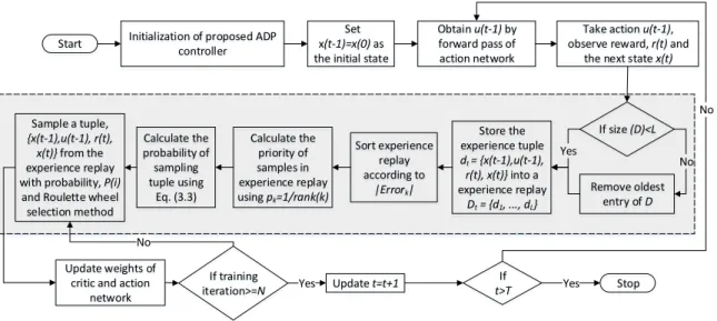
Figure 2.2. The algorithm flowchart of the proposed ADP design. . . 38

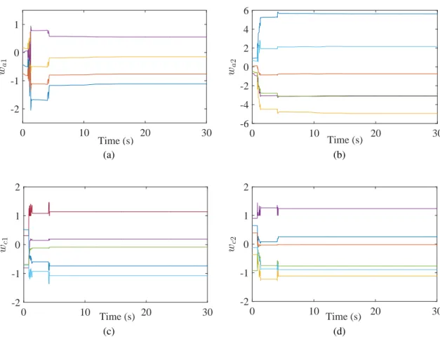
Figure 2.3. The training process of ADP controller: (a) weights trajectories from 4 inputs to 1 hidden node in action network; (b) weights trajectories from 6 hidden to 1 output node in action network; (c) weights trajecto-ries from 5 inputs to 1 hidden node in critic network; and (d) weights trajectories from 6 hidden to 1 output node in critic network. . . 43

(12)

Figure 2.4. The training process of ADP controller: (a) trajectory of output of critic network,J(t); (b) reinforcement signal,r(t); and (c) control ac-tion,u(t). . . 44

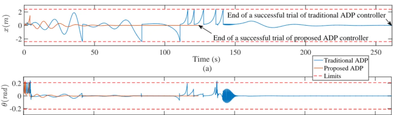
Figure 2.5. Performance comparison between proposed ADP controller and

tradi-tional ADP controller (a)x(m), and (b)θ (radians). . . 45

Figure 2.6. Typical trajectory of proposed ADP controller on the triple-link

pen-dulum balancing task: position of the cart,xfor a successful run. . . . 48

Figure 2.7. Performance comparison between proposed ADP controller and

tradi-tional ADP controller with the convergence of state,x(m). . . 49

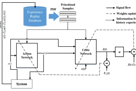
Figure 3.1. Proposed ADP diagram based on prioritized experience replay. . . 55

Figure 3.2. Probability density function for (a) Uniform random sampling (b)

Pri-oritized sampling. . . 56

Figure 3.3. Training procedure for prioritized experience replay based ADP with

prioritized sampling method. . . 58

Figure 3.4. Proposed ADP algorithm based on prioritized experience replay. The

highlighted portion shows detailed steps for prioritized experience re-play integration. . . 60

Figure 3.5. Box plot comparison of two methods: ER based ADP and PER based

ADP with respect to trials to succeed for uniform 10% sensor noise condition. . . 72

Figure 3.6. Typical curves: (a) error curve (b) probability curve with rank

repre-sented by numbers from 1 to 10 for 10 tuples in experience replay with no failure experiences. . . 73

(13)

Figure 4.1. Schematic diagram of VSM current controlled voltage source inverter with closed loop current controller and phase locked loop tracked from the grid. . . 79

Figure 4.2. d-q equivalent model of three-phase inverter with cross-coupling and

feed-forward terms included. . . 81

Figure 4.3. ADP controller used as a supplementary controller (Refer to Fig. 4.1

for implementation in VSM system). . . 83

Figure 4.4. Action neural network with 3 inputs, 6 hidden neurons, and 1 output

neuron. . . 84

Figure 4.5. Critic neural network with 4 inputs, 6 hidden neurons, and 1 output

neuron. . . 86

Figure 4.6. Comparision between ADP and conventional PI Controller. (a) d-axis

reference current signal(I_{dre f}). (b) Overshoot at first step change re-duced with supplementary ADP controller and system response made faster. (c) Overshoot at second step change reduced with

supplemen-tary ADP controller and system response made faster. . . 90

Figure 4.7. Harmonic spectrum of the grid current in the case of PI controller. . . . 91

Figure 4.8. Harmonic spectrum of the grid current in the case of ADP as a

supple-mentary controller. . . 91

Figure 4.9. Schematic diagram of VSM benchmark system connected to grid through

∆-Y transformer and single phase unsymmetrical fault with fault impedance

(14)

Figure 4.10. Three phase inverter output voltages (line to neutral) under single phase unsymmetrical fault at 0.054167 sec and cleared at 0.1 sec. . . 93

Figure 4.11. Ability of supplementary ADP to track I_{dre f} under single phase

un-symmetrical fault at 0.054167 sec and fault cleared at 0.1 sec. . . 94 Figure 4.12. Three phase current with PI controller under single phase

unsymmet-rical fault at 0.054167 sec and fault cleared at 0.1 sec. . . 95 Figure 4.13. Three phase current with ADP controller under single phase

unsym-metrical fault at 0.054167 sec and fault cleared at 0.1 sec. . . 96

Figure 5.1. Microgrid with non-linear loads and shunt active filter connected to

reduce harmonics. . . 98

Figure 5.2. Schematic diagram of a shunt active filter connected to source and

non-linear load for compensation of harmonics. . . 102 Figure 5.3. Current reference generation (i_α_{re f} andi_β_{re f}). . . 103

Figure 5.4. Overall diagram of online learning based ADP controller for the inner

current control loop in the power inverter (Fig. 5.2). . . 109

Figure 5.5. Critic neural network with 8 inputs, 12 hidden neurons, and 1 output

neuron. . . 109

Figure 5.6. The training process of ADP controller: (a) weights trajectories from 6

inputs to 1 hidden node in action network, (b) weights trajectories from 12 hidden to 1 output node in action network, (c) trajectory of output of critic network, J(t), and (d) reinforcement signal, r(t) during the training process. . . 113

(15)

Figure 5.7. Performance comparison between two control techniques: PI and PI+ADP with tracking curve for (a) direct axis current, I_d, and (b) quadrature axis current,Iq. . . 117

Figure 5.8. Control actions generated by ADP for (a) direct axis current,I_d, and

(b) quadrature axis current,I_q. . . 117

Figure 5.9. Dynamic experiment response of the power inverter connected

sys-tem. First figure shows source current with the power inverter (PI controller implemented) connected at 0.11s. Second figure shows proved source current with the power inverter (PI+ADP controller im-plemented) connected at 0.11s. All these currents are for the first A-phase. . . 118

Figure 5.9. Comparative study of PI and PI+ADP controller for (a) Active power

transients, and (b) Reactive power transients because of the power in-verter connected at 0.11s. These figures are zoomed-in to show supe-rior performance of the ADP controller. . . 120 Figure 5.10. Performance comparison of PI and ADP under different loading

con-ditions. . . 121 Figure 5.11. Comparison of dominant harmonics for PI and ADP under load=100W.

(16)

LIST OF TABLES

Table 2.1. Performance evaluation for cart-pole balancing task for 100 runs. The

2nd, 3rd and the 4th column are with the traditional ADP method, while 5th, 6th and 7th column are with our proposed ADP method. . . 42

Table 2.2. Parameters used in the triple-link inverted pendulum benchmark . . . . 47

Table 2.3. Performance evaluation for triple-link inverted pendulum balancing task

for 100 runs. The 2nd, 3rd and the 4th column are with the traditional ADP method, while 5th, 6th and 7th column are with our proposed ADP method. . . 48

Table 3.1. Performance evaluation for cart-pole balancing task for 100 runs. The

2nd, 3rd and the 4th column are with the traditional ADP method, while 5th, 6th and 7th column are with experience replay ADP method. The 8th, 9th and 10th column are with the proposed ADP method. . . 71

Table 3.2. Performance evaluation for triple-link inverted pendulum balancing task

for for 100 runs. The 2nd, 3rd and the 4th column are with the tradi-tional ADP method, while 5th, 6th and 7th column are with experience replay ADP method. The 8th, 9th and 10th column are with the pro-posed ADP method. . . 75

Table 4.1. Performance measurement of d-axis current control corresponding to

Fig. 4.6 . . . 92

Table 4.2. Performance measurement of d-axis current control corresponding to

(17)

(18)

ABSTRACT

INTELLIGENT LEARNING CONTROL SYSTEM DESIGN BASED ON ADAPTIVE DYNAMIC PROGRAMMING

NARESH MALLA 2017

Adaptive dynamic programming (ADP) controller is a powerful neural network based control technique that has been investigated, designed, and tested in a wide range of applications for solving optimal control problems in complex systems. The performance of ADP controller is usually obtained by long training periods because the data usage efficiency is low as it discards the samples once used. Experience replay is a powerful technique showing potential to accelerate the training process of learning and control. However, its existing design can not be directly used for model-free ADP design, because it focuses on the forward temporal difference (TD) information (e.g., state-action pair) between the current time step and the future time step, and will need a model network for future information prediction. Uniform random sampling again used for experience replay, is not an efficient technique to learn. Prioritized experience replay (PER) presents important transitions more frequently and has proven to be efficient in the learning process.

In order to solve long training periods of ADP controller, the first goal of this thesis is to avoid the usage of model network or identifier of the system. Specifically, the

experience tuple is designed with one step backward state-action information and the TD can be achieved by a previous time step and a current time step. The proposed approach is

(19)

tested for two case studies: cart-pole and triple-link pendulum balancing tasks. The proposed approach improved the required average trial to succeed by 26.5% for cart-pole and 43% for triple-link. The second goal of this thesis is to integrate the efficient learning capability of PER into ADP. The detailed theoretical analysis is presented in order to verify the stability of the proposed control technique. The proposed approach improved the required average trial to succeed compared to traditional ADP controller by 60.56% for cart-pole and 56.89% for triple-link balancing tasks. The final goal of this thesis is to validate ADP controller in smart grid to improve current control performance of virtual synchronous machine (VSM) at sudden load changes and a single line to ground fault and reduce harmonics in shunt active filters (SAF) during different loading conditions. The ADP controller produced the fastest response time, low overshoot and in general, the best performance in comparison to the traditional current controller. In SAF, ADP controller reduced total harmonic distortion (THD) of the source current by an average of 18.41% compared to a traditional current controller alone.

(20)

CHAPTER 1 INTRODUCTION

1.1 Background

In literature, reinforcement learning (RL) is defined as the learning about how to map situations to action taken by an agent so as to maximize the reward [1, 3]. A

reinforcement learning task that satisfies the Markov property is called a Markov decision process (MDP). The traditional RL algorithms have great difficulty in evaluating the future optimal actions with huge searching space. Deep learning enables multi-layer processors/perceptrons to learn the data representation with multiple levels of encoding and decoding process. These methods improve the state-of-the-art pattern recognitions (e.g., speech, object, genomics and others) [7]. Deep Q network (DQN), one type of deep reinforcement learning algorithms, has been developed to mimic human and animals’ decision making process through a combination of reinforcement learning and hierarchical sensory processing systems [6, 8–10]. It uses several layers of nodes to build up the mapping and representation of the data and it makes the neural network capable to learn concepts from raw sensory or image data (which is usually with very high-dimension state spaces). Backpropagation algorithm is one of the typical ways to show how such a model adjusts its weight parameters to represent the relationship between input and output [11]. Several different versions of backpropagation algorithms have also been developed to improve the convergent speed for large-scale input data stream [12]. Convolutional neural network (CNN) is another powerful technique to extract represented features and conduct end-to-end policy searching for 2-D images, yet may require certain computation at times [13, 14]. Interesting applications of deep reinforcement learning have been reported

(21)

in robot navigation and robot arm manipulation [15, 16]. Among all the reported results, the deep auto-encoder and certain training algorithms are generally used for this type of large searching space decision making problems. These frontier results also inspired the possible integration to other control and optimization fields.

One class of reinforcement learning methods is based on the actor-critic structure, where an actor generates an action and a critic component evaluates the performance. This principle motivates the development of a family of approximate or adaptive dynamic programming (ADP) designs. There are three typical structures in ADP design family, heuristic dynamic programming (HDP), dual heuristic dynamic programming (DHP) and Globalized dual heuristic dynamic programming (GDHP). They are mainly applied for online control and optimization problems. For example, in HDP design, it consists of an action and a critic networks. The critic network is designed to evaluate the current online learning performance based on the instant control action, while the action network produces an online learning based control signal to improve the control

performance [2, 17–23]. DHP and GDHP are so-called advanced ADP designs, and are expected to learn and control faster and more accurate than the basic HDP design. HDP will be referred to as ADP hereinafter. Depending on whether it needs a model-network or not, ADP methods can also be categorized as model-free design [24–26] and model-based designs [27–30]. In recent years, event-based ADP [31] and data-based ADP [32] are developed to design the adaptive robust control for the nonlinear systems. Many of the theoretical and convergence analysis publications have reported to guarantee the optimal policy after the learning-interaction process [33–36]. However, learning/convergent speed and data efficiency are two of the challenges of applying ADP based methods in

(22)

real-world applications.

Currently, there has been a trend studying the advantages of experience replay technique to improve the data efficiency of ADP/RL methods from both theoretical and experimental perspectives [4, 37–39]. Classical ADP based control converges relatively slow, because it needs enough time to learn to interact with systems. The samples are used only once and then discarded right away. The controller could easily “forget” the previous experience after learning for a long time. Thus, the learning is not efficient and accurate after a long period of time. Some pilot studies with the integration of experience replay have been reported on ADP designs for dc motor, inverted pendulum, and zero-sum games [40, 41]. However, it is still an open question how to systematically facilitate the learning and association process of ADP based approaches in a general way and explore the various real applications.

1.2 Reinforcement Learning and Adaptive Dynamic Programming

In this section, we will first introduce the background and fundamental principles of Markov decision process, and then its optimal solutions based on reinforcement learning and adaptive dynamic programming.

1.2.1 Markov Decision Process

MDP model consists of a set of possible states (s_t), a set of possible actions (a_t), some reward function (R(s_t,a_t)), and a probability that an actiona_t=u(t)in state st=x(t)will lead to next statest+1=x(t+1). Note that in next chapters,xis used to

denote state anduis used to denote control action. MDP must satisfy the Markov property

(23)

depends on that state. For given state,s, next state,s0and actiona, the probability of each possible next state, known as the transitional probability can be defined in a particular finite MDP as [1]:

Pa

ss0 =Pr{st+1=s 0_|_s

t=s,at=a}. (1.1)

The expected value of the next reward,r_t+1can be written as:

Ra

ss0 =E{rt+1|st =s,at =a,st+1=s 0_}_.

(1.2)

The state-value function,Vπ _{for an arbitrary policy}_π _{can be evaluated by cumulating}

future possible discounted reward:

Vπ(s) =E_π{r_t+1+γrt+2+γ2rt+3+...|st =s} (1.3)

=E_π{r_t₊₁+γVπ(st+1)|st=s}. (1.4)

where,r_t+1,rt+2,rt+3, ... are rewards received at timet+1,t+2,t+3...andγ is the

discount factor. The successive approximationV(s)can be obtained by using the Bellman

equation as an iterative update rule:

Vt+1(s) =Eπ{rt+1+γVt(st+1)|st=s}. (1.5)

After following the existing policyπ, we can consider selecting actionain states. Then, the value of this way of behaving is:

(24)

Qπ₍_s_,_a_{) =}_E

π{rt+1+γVπ(st+1)|st=s,at =a}. (1.6)

IfQπ₍_s_,_π0₍_s₎₎_≥_Vπ₍_s₎_{, then policy}_π0_{must be as good as, or better than}_π_{. This is called}

policy improvement process.

1.2.2 Reinforcement Learning

Reinforcement learning is a type of learning in which learner or decision maker known as the agent interacts with its environment to take actions so as to achieve certain goal. The agent is naive at the beginning and is subjected to new situations from which it learns to make decisions so as to maximize cumulative reward from the environment over the time. This basic concept is also illustrated by Fig. 1.1 [1]. At each time stept, the agent observes the state of the environment,s_t, and based on that generates an action,a_t. Meanwhile, it will receive an instant rewardrt, indicating the control performance. The

agent will adjust its parameters to maximize the reward in the future. This process is repeated along the time axis.

Almost all reinforcement learning algorithms are based on estimating value functions, that estimate how good it is to perform certain action in a certain state. The value function of a statesunder an optimal policy, denoted byV∗, is the expected return and can be defined as:

V∗(s) =max a Eπ ∗{R_t|s_t=s,a_t =a} =max a Eπ ∗{_r_t₊₁+_γ ∞

∑

k=0 γkr_t+k+2|st=s,at =a} =max a E{rt+1+γV ∗₍_s t+1)|st=s,at =a}. (1.7)

(25)

Agent

Environment

action at state st reward rt rt+1 st+1

Figure 1.1. Interaction between agent and environment in reinforcement learning (this figure is reprinted from [1]).

whereEπ∗{}denotes the expected value if the agent follows the optimal policyπ∗. The

last equation is one of the form of Bellman optimality equation [42] forV∗. The Bellman optimality equation forQ∗is

Q∗(s,a) =E{r_t₊₁+γmax

a0

Q∗(s_t₊₁,a0)|s_t =s,a_t =a} (1.8)

Reinforcement learning algorithms are usually used to solve the discrete-time

optimization problems with Markov properties. For years, Q-learning, SARSA (λ) and

temporal difference (TD) algorithms are the most commonly used methods for maze navigation, path planning and other agent-environment interaction applications.

1.2.3 Adaptive Dynamic Programming

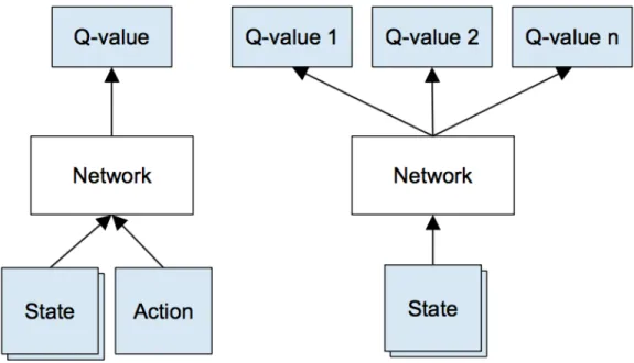
For continuous-time and continuous-state problem optimization with Markov properties, adaptive dynamic programming is one of efficient ways to solve it. Fig. 1.2 shows the actor-critic structure which is based on the reinforcement learning principle. In

(26)

this design, the critic and the actor are tuned online using the observed data containing state variable, reward and next state variable along the system trajectory. Neural networks are typically used to build the mapping of action/critic structure here. Weights of one Globalized neural network (NN) are kept constant while weights of other NN are tuned and the procedure is repeated until both NN have converged. After enough training, the actor produces the optimal control action and critic evaluates the performance of actor over time. Learning and interaction is the key that enables adaptive controller to converge to the optimal control. Neural network, fuzzy logic, and other computational intelligence techniques can be employed to implement the mapping of critic and action networks.

CRITIC–Evaluates

the Current

Control Policy

ACTOR–

Implements the

Control Policy

System/

Environment

Control

Action

System

Output

Reward/

Response

from

Enviroment

Policy

Update/

Improvement

Figure 1.2. Reinforcement Learning with an actor/critic structure [2].

Heuristic dynamic programming is one of the basic ADP designs which only consists of action and critic networks. The architecture of critic network is a multi-layer perceptron (MLP) structure. The inputs to the critic network are the measured system

(27)

state vector,s(t), and control action,a(t). J(t)is the output of the critic element and theJ function approximates the discounted total reward to go.

Adaptive dynamic programming and reinforcement learning are both commonly used in the society for the optimization of decision making process. Though

reinforcement learning can also deal with continuous time systems, it is usually required to discretize the state and action spaces before hand. This may possibly sacrifice accuracy or increase the computational load in some cases. The advantage of adaptive dynamic programming is to deal with continuous state system in continuous time fashion.

1.3 Computational Intelligence Techniques in Online Learning and Optimal Control

In this section, we will discuss the key components in deep reinforcement learning, e.g., deep autoencoder, convolutional neural network, and one of the important parameter to be used for algorithm development in next chapters: termed as experience replay.

1.3.1 Autoencoder and Deep Autoencoder

An autoencoder neural network is with MLP structure which has one or more hidden layers. The input is first encoded by hidden nodes which can be decoded to produce output.

The simplest example of autoencoder can be realized by 8-3-8 network as shown in Fig. 1.3 and Fig. 1.4, rooted from [3]. These results are generated from the authors’ graduate course project: EE792: Computational Intelligence. In the network shown in Fig. 1.3, the eight network inputs are connected to three hidden units, which are in turn connected to the eight output units. Because of this structure, the three hidden units will be forced to represent the eight input values in some way that captures their relevant

(28)

+0.5 Bias Node W1 W2 h1 Inputs (8) Outputs(8) Input Layer Hidden Layer Output Layer X1 X2 X3 X8 Y1 Y2 Y3 Y8

Figure 1.3. 8-3-8 neural network which can be used to learn input and output (this figure is reprinted from [3]).

features, so that this hidden layer representation can be used by the output units to compute the correct target values. The network shown in Fig. 1.3 can be trained to learn the simple output target function:

Out put y=Input x. (1.9)

wherexis a vector containing binary values. The network must learn to reproduce the

eight inputs at the corresponding eight output units. Although this is a simple function, the network in this case is constrained to use only three hidden units. Therefore, the essential information from all eight input units must be captured by the three learned hidden units. When backpropagation is applied to this task, the autoencoder successfully learns the

(29)

Input

10000000

01000000

00100000

00010000

00001000

00000100

00000010

00000001

Output

10000000

01000000

00100000

00010000

00001000

00000100

00000010

00000001

Hidden Values

0.9912 0.9909 0.9957

0.0404 0.2634 0.9828

0.9490 0.9928 0.0072

0.8884 0.0035 0.7604

0.9895 0.2031 0.0159

0.0057 0.9898 0.6685

0.0844 0.4970 0.0077

0.1692 0.0054 0.2037

Figure 1.4. Learned hidden layer representation for 8-3-8 network

target function using the eight possible vectors as training examples. If the number of hidden layer increases, then the autoencoder is called deep autoencoder. Deep

autoencoder finds many applications in image search [43], data compression [44], topic modeling and information retrieval [45]. The training algorithm and neural network structure may be different (e.g, Restricted Boltzmann Machine), however the principle remains the same in case of deep autoencoder [46].

1.3.2 Convolutional Neural Networks

Convolutional neural network (CNN) is a variation of MLPs which is mostly used in deep learning techniques. It consists of one or more convolutional layers followed by one or more fully connected MLP layers. The input to a convolutional layer is with input size as:

(30)

wheren×nis height and width of image in pixels andr=number of channels (e.g.,r=3 for RGB image). The convolutional layer will havekfilters of size as:

Filter size=m×m×q. (1.11)

wherem≤nandq≤r. Within each layer of CNN, set of feature detectors exists, each of

which responds to the presence of a particular pattern in an input tensor [47]. Each filter is replicated across the entire visual field and they share the same weights and bias to form a feature map which increases efficiency. Between layers, dimension reduction technique called max pooling layer [48] or strided convolutions [49] are utilized. Backpropagation algorithm can be used to compute the gradient with respect to the parameters of the model in order to use gradient based optimization [50].

1.3.3 Deep Q Network

Deep Q-network is an artificial agent with ability of recent advances in training deep neural network that can learn successful policies directly from high-dimensional sensory inputs using reinforcement learning [6]. Deep Q-network agent takes only the pixels and the game score as inputs and has learning capability to excel at a diverse array of

challenging tasks. In case of deep Q-network, the compressed feature of deep autoencoder is treated as state and stored in experience replay. At every update iterationi, the current

parametersθ are updated so as to minimize the mean-squared Bellman error with respect

to old parametersθ, by optimizing the following loss function (DQN Loss):

Li(θi) =E[(r+γmax

a0

(31)

For each updatei, a tuple of experience(s,a,r,s0)∼U(D)(or a minibatch of such

samples) is sampled uniformly from the replay memoryD. For each sample (or

minibatch), the current parametersθ are updated by a stochastic gradient descent

algorithm. Specifically,θ is adjusted in the direction of the sample gradientgiof the loss

with respect toθ,

gi= (r+γmax a0 Q(s

0_,_a0_;

θ_i−)−Q(s,a;θi))∇θiQ(s,a;θ) (1.13)

Then, actions are selected at each time-stept by anε-greedy behavior with respect to the current Q-networkQ(s,a;θ)as described in [51].

1.3.4 Experience Replay

Experience replay (ER) technique delivers memory capacity for a learning agent to recall past experiences and apply them to update the current policy. Thus, high data efficiency is achieved by reusing the samples. The basic technique behind experience replay is to store all the experience tuple defined as,

et = (s,a,r,s0) (1.14)

wheret refers to the time instance. The overall replay memory is defined as

(32)

When training the neural network, random minibatches from the replay memory are sampled instead of the most recent transition to avoid local minimum. Experience replay is first proposed in [52], in which experience data are stored and chosen randomly to update the value function and policy in reinforcement learning for neural network approximation. As mentioned in [53], the advantages of experience replay are twofold, first it helps to increase the sample efficiency by allowing samples to be reused. On top of this, in the context of neural networks, experience replay allows for mini-batch updates which helps the computational efficiency, especially when the training is performed on a GPU. In addition, learning from mini-batch samples would cause the updates of the network parameters to have a low variance, leading to faster and potentially more stable learning. Second advantage is that the experiences used to train the networks are not only

based on the most recent policy andε can be used to scale the amount of exploration. If

ε=1, the movement is completely random and ifε=0, the best policy is followed i.e., greedy behavior. Use of past experiences and past policy also avoids the algorithm getting stuck in a local minimum or diverging case [6].

1.4 Discussion of Opportunities for Deep Learning Enabled Adaptive Dynamic

Program-ming

Deep reinforcement learning and experience replay methods open many new opportunities for adaptive dynamic programming in the continuous time and continuous state domain. “End-to-end” learning and control from raw images or sensory data to the optimized control action is also possibly solvable by the deep learning enabled ADP approach. Feature representation, deep auto-encoder, convolutional neural network, and

(33)

deep Q network are the possible necessary components for deep learning enabled ADP design. Currently, there are also a few pilot studies on applying experience replay to improve the learning and data efficiency of ADP approach for zero-sum optimization problem.

In [54], an actor-critic, model-free algorithm based on the deterministic policy gradient is presented that can operate over continuous action spaces. Using the same learning algorithm, network architecture and hyper-parameters, their algorithm robustly solved more than 20 simulated physics tasks, including classic problems such as cartpole swing-up, dexterous manipulation, legged locomotion and car driving. Similarly, [55] applied the deep Q-network on standard RL testing continuous as well as discrete domains, such as grid world, mountain car problem, and inverted pendulum problem. Training neural network with the recent data causes it to forget previous data and learning will be difficult. Thus, experience replay plays a vital role in convergence of neural network of deep reinforcement learning whose integration in ADP controller is at its pilot stage. The experience replay was integrated in [40] to update the weights of the action network and critic network in ADP approach [24] for optimal control of DC motor problem [56] and inverted pendulum.

1.4.1 Feasibility for Integration of Experience Replay for RL Structure

An integral reinforcement learning and experience replay algorithm is developed on an actor-–critic structure in [37] to learn online the solution to the

Hamilton–Jacobi-Bellman equation for partially-unknown constrained-input systems. The near optimal solution convergence and stability was guaranteed in this paper with ER

(34)

based RL framework. The authors proposed one way to integrate experience relay based gradient-descent algorithm for tuning the weights of critic NN by using the current data and some past data (which are stored but can be removed and replaced) for learning the weights at each specific time. This can be observed in Eq. (28) and Eq. (42) of the paper [37]. They also stated that new data points can replace old ones in the history stack, only if a replacement increases the minimum eigenvalue and consequently increases the convergence rate of the critic NN weights. This implies that tuning weights of critic network with experience replay updating law improves the convergence speed. In the meawhile, the authors only used a single-layer NN for each actor-critic structure.

In [57], ER in actor-critic algorithm is proposed to address the issues of efficiency and autonomy that are required to make reinforcement learning feasible for real-world control tasks. Their experimental study with simulated octopus arm and half-cheetah demonstrates the practicability of the proposed algorithm to solve difficult learning

control problems in a reasonable short time. A general ER framework is developed in [38] that can be combined with essentially any incremental RL technique, and instantiates this framework for the approximate Q-learning and SARSA algorithms. Authors also present promising real time learning results in inverted pendulum and robot systems, which are encouraging for real time applicability.

1.4.2 Maze Navigation Problem

Maze navigation problem is an interesting example for understanding deep reinforcement learning principle. The state of the environment in maze navigation

(35)

coordinate position as states but it may not be universal in other games. Thus, the authors in [12] take screen pixels containing sufficient information about maze navigation

problem. Raw pixels are also used as input state of a reinforcement learning problem in using fitted Q-iteration to generate optimal policy. The first step in deep reinforcement learning is preprocessing the image and compressing it to lower dimension using deep autoencoder. Processing the benchmark dataset MNIST, a deep autoencoder as described in [46] could be trained and tested using the backpropagation algorithm as mentioned in [3]. In [12], the preprocessing technique is applied first: taking screenshot, resizing them to 30x30 pixels and converting to grayscale with 256 gray levels. 6200 of these images were taken, 3100 are used for training and 3100 for testing. These images are then feeded to 900-900-484-225-121-113-57-29-15-8-2-8-15-29-57-113-121-225-484-900-900 deep autoencoder structure. This deep autoencoder is retrained and fine-tuned until they get the reconstruction for testing images exactly same as input similar to method as shown in Fig. 1.5.

Deep reinforcement learning perfectly fits into this situation as we could represent our Q-function with a neural network, that takes the state (compressed 2 dimensional hidden layer values) and output Q-value for each possible action (1:right, 2:up, 3:left, 4:down). If the agent reaches the goal, reward is set as 1 else reward is 0. Resilient backpropagation proposed in [58] is used in [12] for training of NNs which is one of the fastest weight update mechanisms. It takes into account only the sign of the partial derivative over all patterns (not the magnitude), and acts independently on each weight factor.

(36)

Figure 1.5. Deep Reinforcement Learning applied to visual control of a racing slot car [4].

1.4.3 Human Level Control

Significant progress has been made by integrating advances in deep learning for image pixels preprocessing and deep autoencoder with reinforcement learning, resulting in the deep Q network algorithm [6] which is capable of human level performance on many Atari video games with only raw pixels as input. Traditionally, DQN is implemented using state and action as the input to the network and the maximum discounted future reward by performing actionain states(Q-value) is obtained as output. In the paper [6], a new deep Q-network is proposed to learn from represented features from raw images as shown in the right side of Fig. 1.6 for each possible action as mentioned in [5]. The advantage of this approach is that to identify the action with the highest Q-value, we only have to do one forward pass through the network and all Q-values for all actions are available immediately. To do so, convolutional neural network can be used for generating

(37)

actions as shown in Fig. 1.7. The network architecture is for 84x84 pixel image and the memory sizes are provided in Fig. 1.8. It shows a classical convolutional neural network with three convolutional layers, followed by two fully connected layers.

Figure 1.6. Schematic illustration of the DQN structure. Left: Naive formulation of DQN. Right: DQN structure used in Deepmind paper [5].

In [51], the first massively distributed architecture for deep reinforcement learning is presented which is applied to 49 out of Atari 2600 games in the Arcade Learning

Environment, using identical hyper-parameters and its performance surpassed non-distributed DQN in above 80% of games. In [59], a conceptually simple and lightweight framework for deep reinforcement learning is proposed that uses

asynchronous gradient descent for optimization of deep neural network controllers. It demonstrated that learning a predictive model of state dynamics can result in a pretrained hidden layer structure that reduces the time strongly required to solve reinforcement learning problems. The neural networks are trained in these literatures by rmsprop weight updating mechanism [60], which is a variant of rprop algorithm [58] used for mini-batch

(38)

Figure 1.7. Schematic illustration of the convolutional neural network [6].

training.

1.4.4 Future Directions

There are still some open questions and challenges along this direction. For example, after the integration of experience replay technique, how to make sure that the computation and calculation will finish within a short sampling time from the algorithm perspective itself. Especially when the size of history stack increases (e.g., [3]), the computation for each time step will certainly increase dramatically. High-performance computational hardware will be strongly required to make sure the controller still finishes the calculation on time. Also, how to systematically select a batch of samples from history stack rather than doing random sampling. The questions and challenges also reveal many opportunities for the fundamental research in this area.

(39)

Figure 1.8. Convolutional neural network with three convolutional layer [5].

1.5 Contributions and Organization of This Thesis

1.5.1 Contributions

The main contributions of this thesis are stated below:

(a) Successfully integrated the history experience for training both the critic and action networks of the ADP controller. The integrated architecture focusses on improving the training speed and adapting to the system faster. The key parameters in the proposed ADP controller are successfully validated online for the different control benchmarks.

(b) Successfully integrated the history experience based on prioritized sampling for tuning weights of both critic and action network of ADP controller. A systematic approach is proposed to integrate history experience in both critic and action networks of ADP controller design.

(c) Experience replay is designed with the backward TD technique to ensure the model-free learning performance of the ADP controller. The model-free ADP design does not rely on an accurate mathematical model of the system. The

(40)

step and the future time step and will need a model network for future information prediction.

(d) Detailed theoretical analysis is presented using Lyapunov theory in order to verify the stability of the proposed control technique.

(e) Application of ADP controller for transient and steady state performance improvement in virtual synchronous machine (VSM). Generally used

proportional-integral (PI) controller in VSM has limited transient performance in current control. ADP controller has been proposed as a supplementary controller for fine tuning conventional PI current controller thereby improving the performance of VSM.

(f) Application of ADP controller for reduction of harmonics in current controlled voltage source inverters. A multiple-input multiple-output (MIMO) online learning control system is developed based on the ADP design. A series of time-delayed current error signals are designed as input for the ADP controller, which outputs compensating control actions (one is for d-axis and the other one is for q-axis) for the current controller in the power inverter. In addition, an appropriate

reinforcement signal has been designed with the delayed tracking errors in the power inverter. Based on this, the ADP controller will generate compensating control actions, which guarantees its success.

1.5.2 Thesis Outline

This thesis has been organized as follows: Chapter 2 highlights the first project with the background of history experience with some of its key features, describes the design of

(41)

Intelligent Learning Control System Design based on Adpative Dynamic Programming

New Adaptive Dynamic Programming

Architectures Smart Grid Applications

Project#1

Design of History Experience Replay for Model Free

Adapative Dynamic Programming Controller

Project#2

Integration of Prioritized Experience Replay Design for

Model Free Adaptive Dynamic Programming with

Stability Analysis

Project#3

Supplementary Adaptive Dynamic Programming

Controller for Virtual Synchronous Machine

Project#4

Harmonic Reduction using Shunt Active Filter and

Online Learning based Control

Figure 1.9. Overall organization of the thesis.

the proposed ADP controller and its implementation flowchart, gives the simulation results from two case studies: cart-pole balancing problem and triple-link inverted pendulum, and concludes the chapter along with some future directions along this work. Chapter 3 introduces the second project with prioritized experience replay and its importance for improvement of convergence of online learning control. The systematic integration technique, stability analysis and experimental results are presented as well. Chapter 4 presents the validation of ADP controller for improvement of performance of traditional PI based current controller in VSM. Chapter 5 presents the validation of ADP controller for harmonic reduction based on current controlled voltage source inverter. The benchmark description is presented along with detailed design procedure and

experimental results. Finally, Chapter 6 presents the conclusion, limitations, and future developments related to the research thesis.

(42)

CHAPTER 2 Design of History Experience Replay for Model Free Adaptive Dynamic Programming Controller

This chapter deals with the new algorithm development and verification with the integration of experience replay. As mentioned in the previous chapter, reinforcement learning (RL) is the learning process of how to map situations to actions taken by an agent so as to maximize the reward [1]. An RL task that satisfies the Markov property is called a Markov decision process. Deep reinforcement learning is a recent advancement in RL tasks which achieved human level performance in Atari video games just by observing the screen pixels and receiving rewards from the game score [8]. The research on deep

reinforcement learning has been growing ever since [6, 51, 54, 61]. One of the important elements that accelerated the convergence and speed up the training of deep reinforcement learning is history experience, also known as experience replay in these papers. History experience delivers memory capacity for a learning agent to recall past experiences and apply them to update the current policy. It stores the sample of experiences and repeatedly presents them to the deep reinforcement learning algorithm. This increases the data efficiency of the system because of the opportunity to reuse past experiences.

An adaptive dynamic programming (ADP) controller is one type of actor-critic structure which can solve optimal control problems in complex decision making systems. It consists of action and critic neural networks (NN) with a multi-layer perceptron (MLP) structure in general. The critic network is designed to evaluate the current online learning based controller while the action network produces an online learning based control signal to improve the control performance [17, 18, 23, 24, 62, 63]. Q-learning and ADP are with

(43)

good convergent properties and have been recently used as well to tackle the single-agent RL task without full information of the system dynamics [64, 65]. ADP controller has shown promising results on a number of power system control examples [66–68]. However, the performance of the ADP controller is usually obtained by long training periods. In other words, traditional ADP based control has a relatively slower convergence rate because it needs enough training to learn to interact with systems. The samples are used once and then discarded. The controller could forget the past experience after training for a long time. Thus, the training is not data efficient and accuracy is low. Following the trend of integrating history experience with reinforcement learning, several papers [38, 57] have shown interesting results by integrating a history experience table into the ADP/RL methods for improving its data efficiency from both theoretical and experimental perspectives. The authors in [37] proposed one way to integrate history experience with a gradient-descent algorithm for tuning the weights of critic NN by using the current data and some past data (which are stored but can be removed and replaced) for learning the weights at each specific time. The improved convergence speed was achieved, however, the experience replay is used to update only the critic weights and the performance improvement by updating both action and critic network weights is not mentioned. In [57], history experience in actor-critic algorithm is proposed to address the issues of efficiency and autonomy that are required to make reinforcement learning feasible for real-world control tasks to solve difficult learning control problems in a reasonably short time. Authors in [38] developed a general history experience framework that can be combined with essentially any incremental RL technique and present

(44)

encouraging for real time applicability. Data in the history experience database is

repeatedly used in [40] to update the weights of the action network and critic network in the ADP approach for optimal control of a DC motor problem [56] and an inverted pendulum. The training speed is improved compared to the traditional ADP approach. The integration of history experience has been reported on actor-critic designs for nonzero-sum games [41]. However, these literatures which integrated history experience in ADP or actor-critic structure or deep reinforcement learning used a one time-step forward sample to train their network which requires a model network to predict the future state. Thus, to systematically facilitate the learning and association process of ADP based approaches by integrating history experience is missing. In addition, maintaining the model-free online learning capability of the integrated approach is also missing for various real-world applications.

There are several major approaches to analyze the stability of the ADP controller. In the learning process, two networks are tuned simultaneously and the stability of the closed-loop system is guaranteed using Lyapunov energy-based techniques [2, 69]. Detailed Lyapunov stability analysis of the ADP based controller is presented in [70] to support the ADP structure from a theoretical point of view. The authors demonstrated that the auxiliary error and the error in the weights estimates are uniformly ultimately bounded (UUB) using the Lyapunov stability construct. In [71], proportional-integral-derivative (PID) control rule is incorporated into neural networks and new results of UUB are provided using a Lyapunov stability construct. The monotonic convergence of optimality is discussed for the goal representation ADP control design in [72], and theoretical proof of convergence is given in terms of both the internal reinforcement signal and the

(45)

performance index. In [73, 74], stability of the ADP controller is presented, where the authors demonstrated the theoretical analysis that the estimation errors of NN weights are UUB by the Lyapunov stability construct. Experimentally, later in simulation section, it can be observed that the weights and parameters of the ADP controller are quickly converged and bounded after the system transients.

Modares et. al. [37] proposed the experience-replay based online algorithm for concurrent learning along with current data for adaptation of critic weights. The

successful real-time learning results presented in [38] are encouraging for further research in experience replay for the real-time reinforcement learning control. A Lyapunov

stability analysis of the ADP based controller is presented in [37] to support the

actor-critic structure with integrated experience replay. The authors used the Lyapunov stability construct to guarantee the success of the overall system. An integral

reinforcement learning and experience replay algorithm is discussed in [75] to show the convergence of the learning process. An analysis of the experience replay is presented in [76] with the theoretical analysis and the effects of replayed and backward TD. It is shown in [77] that the estimation bias is bounded and asymptotically vanishes, which allows the actor-critic and experience replay based algorithm to preserve the convergence properties of the original algorithm. All these existing publications provide guidance to derive the theoretical stability analysis for the proposed ADP design.

All of aforementioned literature motivates the research to integrate the powerful learning capability of history experience to ADP. However, the existing design of history experience cannot be directly integrated into a model-free ADP design. It is because the existing work uses the forward temporal difference (TD) information (e.g., state-action

(46)

pair) between the current time step and future time step to train the network. To predict the future state-action pair, the model network or identifier of the system/environment is essential. In such case, offline data is needed to build the model network and train it very well. The advantage of the backward TD information used in the history experience replay design in this chapter is to avoid the usage of the model network or identifier of the system/environment. Thus, this chapter proposes a systematic history experience replay design to avoid the model network usage. Specifically, the history experience is designed with the tuple or sample from the current time step,t, and the previous time step,t−1. Thus, the TD can be achieved by the previous time step and the current time step and experience tuple is designed with a one step backward state-action pair. This preserves the model-free online learning capability of the ADP method. The major contributions of this chapter are twofold:

1. The project in this chapter has integrated the history experience for training both the critic and action networks of the ADP controller. The integrated architecture

focusses on improving the training speed and adapting to the system faster. The key parameters in the proposed ADP controller are successfully validated online for the different control benchmarks.

2. The history experience is designed in this chapter with the backward TD technique to ensure the model-free learning performance of the ADP controller. The

model-free ADP design does not rely on an accurate mathematical model of the system. The traditional forward TD technique (e.g., state-action pair) is between the current time step and the future time step and will need a model network for future

(47)

information prediction.

In addition, the performance improvement is verified with the help of two control problems: a cart-pole balancing task and a triple-link pendulum balancing task. The integration of history experience improves the data efficiency and preserves the online learning capability of the ADP. For fair comparison, we set the same initial starting states and initial weight parameters for both approaches (traditional ADP and history experience integrated ADP) under the same simulation environment. The triple-link pendulum is considered to be one of the most difficult and challenging balancing tasks. Our proposed controller has balanced the system in a short time when the traditional ADP is still at its learning phase.

2.1 Background of History Experience

This section presents the background of history experience starting with the batch training method. The benefits of history experience are then discussed and the time complexity of using this method are focussed at the end.

2.1.1 Batch Learning

Batch reinforcement learning is defined as the task of learning the best possible policy from a fixed set of a transition samples, known as a batch, which can be easily adapted to the classical online case where the agent interacts with the environment while learning. It is a subfield of dynamic programming-based reinforcement learning [78]. Batch learning is one of the methods to learn from the history experience. The idea behind history experience for batch learning is to speed up convergence by using observed state transitions once and reusing them repeatedly as if they were new observations. The

(48)

transitions collected using history experience reflect the connection between the states. By spreading it along these connections, there is more efficient use of this information. One of the fastest methods to efficiently learn from these batches of samples is a resilient back-propagation algorithm [12, 58]. However, the algorithm complexity makes it difficult for online learning implementation [79] and thus the gradient descent algorithm is

commonly used in the literature. One major difference between batch and online learning is that the batch algorithm computes the error associated with each input sample while keeping the system weights constant. However, online learning updates system weights for each sample in the input. At the end, both algorithms usually converge to the same global minima.

2.1.2 Benefits of History Experience

In addition to increase in data efficiency of the system, another beneficial effect of history experience is the aggregation of information from multiple trajectories as

explained in [38]. For an example of a cart-pole, the trajectory to successfully balance a pole may be different. If more than one trajectory are used to train the actor-critic structure during the online process instead of only current data, the convergence will be faster and will be verified later. The other benefit of history experience is that it

asymptotically has similar effects with eligibility traces. This is because it transmits similar information as propagated by the eligibility traces [38]. To collect the past information, eligibility traces can be used to provide a short-term memory of many previous input signals. The addition of eligibility traces can accelerate the TD learning process. λ is an eligibility trace decay parameter which normally lies in the range [0,1].

(49)

Here, 0 represents no eligibility traces. The benefit of an eligibility trace without having to tune the additional parameter,λ, is obtained with increased size of history experience.

History experience breaks the temporal correlations of the neural network learning updates. It also makes sure that the experiences used to train the networks are not only

based on the most recent policy andepsiloncan be used to scale the amount of

exploration. This makes sure the algorithm won’t get stuck in a local minimum or diverge. The neural networks are global function approximators and online learning might cause the network to forget when learning a new task, even if it has previously learned to do the related task well. Thus, it is important for the neural networks to properly generalize their knowledge to the whole state-action space by varying the training data enough in the experience database [53].

2.1.3 Discussion of Time Complexity

The most computationally demanding component of the history experience integrated algorithm is the weight updating part, which consumes certain time to reduce the error below the threshold. Parallel computing techniques in a recent simulation environment solves high computational and data-intensive problems using multicore processors, GPUs, and computer clusters. The weights updating part for the action and critic networks by history experience can be implemented using a parallel computing toolbox which divides the computation among available workers. This would reduce the computation time and improve the performance of the system. With the recent

advancement in modern technology, the computation burden may not be a barrier for new processors. Thus, a history experience integrated algorithm can have a less computational

(50)

burden and have the potential to provide real time optimal control action.

2.2 Proposed ADP Controller and Implementation

This section presents our method of improving the training mechanism of the ADP using history experience along with design and implementation details. The stability of the ADP controller is discussed as well. The proposed algorithm stores the sample of experiences and repeatedly presents them to a gradient-descent based online ADP training algorithm. This increases the data efficiency of the system due to reuse of the otherwise discarded samples.

2.2.1 Overall Framework

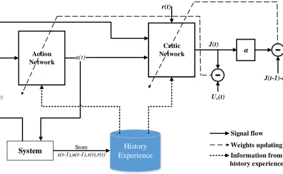
The overall diagram of the proposed ADP controller design based on history experience is shown in Fig. 2.1. The proposed controller is a model-free technique that does not require a model network and can adapt to any system to which it is connected to. In one of the basic ADP designs, known as heuristic dynamic programming (HDP) [24], the action network generates the optimal control action iteratively and a critic network

evaluates the performance of the action network by approximatingJclose to the optimal

solution. Jis also the output of the critic network. The controller observes the state,x(t)

from the system and generates the action,u(t)by interacting with the action network. The basic idea in adaptive critic design is to adapt the weights of the critic network to

approximate the optimal cost function,J∗(x(t)), satisfying the modified Bellman principle of optimality [42], given by:

J∗(x(t)) =min

u(t){

(51)

The optimal online learning based controller can be written as:

u∗(x(t)) =argmin

u(t)

J∗(x(t)) (2.2)

wherex(t)is the input state vector,r(x(t))is the immediate cost incurred byu(t)at time t, andUcis the ultimate desired objective which the cost function is desired to achieve. This

equation cannot be analytically solved in general. Adaptive dynamic programming is one of the efficient ways to iteratively solve continuous-time and continuous-state problem optimization. X 2 X 1 X 3 h 3 h 2 h 4 h 5 h 6 h 1 u X2 X1 X3 h 3 h 2 h 4 h 5 h 6 h 1 J u System J(t) α Action Network Critic Network Uc(t) Signal flow History Experience Store x(t-1),u(t-1),x(t),r(t) x(t) u(t) r(t) Weights updating Information from history experience J(t-1)-r(t)

Figure 2.1. The architecture of the proposed ADP controller design with history experience memory.

(52)

2.2.2 Design of Model-Free History Experience

The measured history data in form of experience tuple:

d(t) ={x(t−1),u(t−1),r(t),x(t)} (2.3)

is stored into the history experience,

D={d(1),d(2),d(3), ...,d(L)}, (2.4)

whereLis the size of history experience. The entire history experience is limited to the size of length,Land the oldest tuple is discarded if the size of history experience increases over the limit. The system is set one time step back to make the controller learn online. Thus, for the first time step, the controller waits and starts training at the next time step. Feedback to the controller is given through a reinforcement signal,r(t)and the next state is observed through taking action,u(t−1). A random tuple is chosen from the history experience to train both the action and critic network as depicted by “Information from history experience” in Fig. 2.1. Here, the random tuple is chosen to break the correlation between the consecutive samples so as to avoid the local minimum [8]. Thus, a tuple of experience,d(t)given by Eq. (2.3) is stored in the history experience,Dgiven by

Eq. (2.4), which will be used to train both the action and the critic network. There are two paths to tune the parameters of action/critic networks in ADP which will be discussed below.

(53)

2.2.3 Design of Critic Network

The architecture of the critic network is a MLP structure. The output of the critic network,Jfunction, approximates the discounted total reward to go. At time,t, the measured system state vector,x(t), and control action,u(t)from the action network are inputs to the critic network, andJ(t)is the output of the critic element. R(t)is the future accumulative reward-to-go value at timet andr(t)=external reinforcement value att. In

the ADP design, theJfunction is used to approximateR(i.e. J→R). The weight

updating mechanism in ADP for the critic network is based on gradient descent rule which minimizes the prediction error for the network given by:ec(t) =αJ(t)−[J(t−1)−r(t)]. The reinforcement signal,r(t)may be as simple as either a “0” or “-1” corresponding to

“success” or “failure” respectively and is provided by the external environment andα is

the discount factor. A tuple of experience, given by equation (2.3), is randomly chosen from the history experience. Then, the inputs to the critic network are the measured system state vector,x(t−1), and control action,u(t−1). J(t−1)is the output of the critic element at time,t−1.

The following weights updating rule is presented to investigate the weights adaptation in the critic network:

wc(t+1) =wc(t) +∆wc(t) (2.5) ∆wc(t) =−lc(t) ∂Ec(t) ∂wc(t) − N−1

∑

n=1 l_c(t) ∂Ecn(t) ∂wcn(t) . (2.6) ∂Ec(t) ∂wc(t) = ∂Ec(t) ∂J(t) ∂J(t) ∂wc(t) (2.7)

(54)

The indexnis used to refer to thenth sample data(n=1, ...,L)stored in the history experience and the time,t, is used for the current time. Note in equation (2.6), the first term is a traditional gradient-descent updating law to minimize the objective function, E_c(t) =0.5e_c(t)2. The last term of equation (2.6) tries to minimize this objective function from the stored samples in the history experience.

2.2.4 Design of Action Network

The action network in the ADP has a similar MLP NN architecture as the critic network. However, the input neuron and output neuron numbers are different. The

principle of adjusting the weights of the action network is to indirectly back-propagate the

error between the approximateJfunction from the critic network and the desired ultimate

objective, denoted byU_c. In turn, the action network can be implemented by either a linear or a nonlinear network depending on the complexity of the problem. The weight updating in the action network can be formulated as follows:ea(t) =J(t)−Uc(t). The ultimate

objective here is to minimize the squared error by adjusting the action network weights. The input to the action network is the measured system state vector,x(t), from a tuple of experience,d(t), randomly chosen from the history stack as described in the previous subsection. The output of the action network is the control action,u(t). The similar weight updating rule as in the critic network can be applied to action network as follows:

wa(t+1) =wa(t) +∆wa(t) (2.8) ∆wa(t) =−la(t) ∂Ea(t) ∂wa(t) − N−1

∑

n=1 l_a(t) ∂Ean(t) ∂wan(t) . (2.9) ∂Ea(t) ∂wa(t) = ∂Ea(t)