Statistics in large galaxy redshift surveys

(1)

Statistics in large galaxy redshift surveys

STOTHERT, LEE,JOHN

How to cite:

STOTHERT, LEE,JOHN (2018) Statistics in large galaxy redshift surveys, Durham theses, Durham University. Available at Durham E-Theses Online: http://etheses.dur.ac.uk/12891/

Use policy

The full-text may be used and/or reproduced, and given to third parties in any format or medium, without prior permission or charge, for personal research or study, educational, or not-for-prot purposes provided that:

• a full bibliographic reference is made to the original source • alinkis made to the metadata record in Durham E-Theses

• the full-text is not changed in any way

The full-text must not be sold in any format or medium without the formal permission of the copyright holders. Please consult thefull Durham E-Theses policyfor further details.

Academic Support Oce, Durham University, University Oce, Old Elvet, Durham DH1 3HP e-mail: e-theses.admin@dur.ac.uk Tel: +44 0191 334 6107

(2)

Statistics in large galaxy redshift

surveys

Lee Stothert

A Thesis presented for the degree of

Doctor of Philosophy

Institute for Computational Cosmology

Department of Physical Sciences

University of Durham

England

(3)

Lee Stothert

Abstract

This thesis focuses on modeling and measuring pairwise statistics in large galaxy redshift surveys. The first part focuses on two point correlation function measure-ments relevant to the Euclid and DESI BGS surveys. Two point measuremeasure-ments in these surveys will have small statistical errors, so understanding and correcting for systematic bias is particularly important. We use point processes to build catalogues with analytically known two point, and for the first time, 3-point correlation func-tions for use in validating the Euclid clustering pipeline. We build and summarise a two point correlation function code, 2PCF, and show it successfully recovers the two point correlation function of a DESI BGS mock catalogue. The second part of this thesis focuses on work related to the PAU Survey (PAUS), a unique narrow band wide field imaging survey. We present a mock catalogue for PAUS based on a physical model of galaxy formation implemented in an N-body simulation, and use it to quantify the competitiveness of the narrow band imaging for measuring novel spectral features and galaxy clustering. The mock catalogue agrees well with ob-served number counts and redshift distributions. We show that galaxy clustering is recovered within statistical errors on two-halo scales but care must be taken on one halo scales as sample mixing can bias the result. We present a new method of de-tecting galaxy groups, Markov clustering (MCL), that detects groups using pairwise connections. We explain that the widely used friends-of-friends (FOF) algorithm is a subset of MCL. We show that in real space MCL produces a group catalogue with higher purity and completeness, and a more accurate cumulative multiplicity function, than the comparable FOF catalogue. MCL allows for probabilistic con-nections between galaxies, so is a promising approach for catalogues with mixed redshift precision such as PAUS, or future surveys such as 4MOST-WAVES.

(4)

Declaration

The work in this thesis is based on research carried out by Lee Stothert under the supervision of Dr Peder Norberg and Professor Carlton Baugh at the Institute for Computational Cosmology, the Department of Physics, Durham, England. No part of this thesis has been submitted elsewhere for any other degree or qualification. Parts of this thesis are the author’s contributions to published work.

• Some of the work in Chapter 2 was used by the Euclid Consortium Internal Documentation as part of the validation of the clustering processing functions.

• Section 3.5 of Chapter 3 reports on work presented in Smith et al. (2018).

• Chapter 4 is published in Stothert et al. (2018).

The figures in this thesis are created by the author unless stated otherwise in the figure caption.

Copyright c 2018 by Lee Stothert.

“The copyright of this thesis rests with the author. No quotations from it should be published without the author’s prior written consent and information derived from it should be acknowledged”.

(5)

I would first like to thank my family. Mum, Dad and Bob have been there to help at every stage of my studies, lending an ear, giving me advice or helping me move. I have always felt supported, and for that I am forever grateful.

I would like to thank Guinevere for patiently listening to my ramblings about my work. She has brightened every day, and I hope she will continue to put up with me and brighten many more.

I am heavily indebted to my two supervisors Peder and Carlton. Without their guidance this work would not have been possible. Their time and effort has been greatly appreciated, and watching and learning from them has made me a far better researcher.

I would also like to thank anyone at the ICC and in the PAUS or Euclid collab-orations who has helped me along the way. I also thank STFC for sponsoring this work.

(6)

Chapter 1

Introduction

1.1

Theoretical models of cosmology

The field of cosmology is the study of the evolution of the Universe. This includes the beginning of the Universe, the formation and growth of structure, and the eventual fate of the universe. It is important to understand the rules and laws that govern this evolution. This section will provide a brief overview of theoretical cosmological models with a focus on the dominant model, ΛCDM.

The majority of cosmological models assume the cosmological principle. This states that on large enough scales (typically more than a few hundred Mpc1_{) the}

universe can be considered to be homogeneous (invariant with regards to position) and isotropic (invariant with regards to direction). This assumption allows for the temporal evolution of the universe on large scales to be described by a single scale factor a(t), which increases (decreases) as the universe expands (contracts). The value of the scale factor at the present timet0is set to unity. Most models, including

ΛCDM, are specific examples of the big bang cosmological model. In the big bang model the early Universe had a very small value ofa(t) and expanded over the age of the Universe to the size it is today, and is currently still expanding.

Gravity is the dominant force on large scales in the Universe. Einstein’s equations

1_{1 pc is defined as the distance at which 1 astronomical unit (roughly the distance from the}

(11)

of general relativity provide accurate predictions for gravitational interaction in the local solar system. If the universe is homogeneous these equations must hold on similar scales in similar environments throughout the universe. A viable model of gravitational interaction on large scales must either be general relativity, or provide a mechanism to sufficiently recover these equations in environments similar to the solar system. The ΛCDM model assumes general relativity to be the correct model of gravitational interaction. Attempts at discovering other viable models of gravity defines the field of modified gravity (Koyama, 2016).

The CDM in ΛCDM stands for cold dark matter. This model assumes cold dark matter is the dominant mass contribution in the Universe. Cold dark matter is a fluid that interacts gravitationally, and only weakly through the other fundamental forces of nature. The prefix cold means that we are assuming that this fluid is non-relativistic, i.e. dark matter particles move at speeds significantly slower than the speed of light. Other models of dark matter can include stronger interactions (Tulin & Yu, 2018) or warm dark matter (Viel et al., 2013).

The Λ of ΛCDM represents the cosmological constant, which is associated with a vacuum energy (or dark energy) that attempts to explain the apparent accelerated expansion of the universe. If we model this dark energy as a perfect fluid, the density ρof the fluid is related to the scale factor of the universe a(t) by

ρ∝a(t)−3(1+w), (1.1.1)

where the value of w, the equation of state parameter, will vary depending on the physical nature of this fluid. A value ofw <−1/3 will lead to an accelerated expan-sion. A true cosmological constant is a special case of this general dark energy model in which the vacuum pressure and density is invariant with changing scale factor of the universe (w=−1). The ΛCDM model assumes that dark energy acts as a cos-mological constant. As the densities of matter (relativistic and non-relativistic) and spatial curvature fall as the universe expands, Λ will be the dominant contribution to the energy density at late times in an expanding universe.

While we assume the universe to be homogeneous on large scales, there is rich structure on small scales. This structure has all formed from small inhomogeneities in the early universe seeded by inflation (Linde, 2014). Gravity caused the overdense

(12)

1.2. Observational cosmology 3

regions of the universe to grow and eventually collapse into the first dark matter halos. Baryonic matter would collect at the centre of these halos due to radiative cooling. Conservation of angular momentum caused these cooling baryons to form into disks, and eventually the first stars and galaxies. From here these small struc-tures began to grow and merge with each other to form larger strucstruc-tures, a process called hierarchical growth. During this process of structure growth, the complex physics of galaxy formation produces the wide variety of structure we can see in the universe. These processes include gas hydrodynamics, star formation and evolution, feedback from supernova and black holes and the dynamics of galaxy interactions and mergers. Many of these processes remain poorly understood, so galaxy surveys like the ones presented here, particularly the Physics of the Accelerating Universe Survey (PAUS), are needed to understand how galaxy properties are related to their host halos.

1.2

Observational cosmology

Observational cosmology aims to observe the real universe to place constraints on the theoretical models of cosmology and the astrophysics of galaxy formation.

1.2.1

Galaxy imaging

Galaxy imaging is typically done using band pass filters. A band pass filter only allows a certain wavelength range to pass. Figure 1.1 shows the filter response curves for the broad band filter set (u, g, r, i, z and Y) of the PAU Camera at the William Herschel Telescope in La Palma (Padilla et al., 2016). This is a very common filter set, overlapping with the near UV, optical and near infrared parts of the spectrum. These broad band filters are typically of the order of 1000˚A in width.

Different filters can correlate with different properties of galaxies. For example, redder filters may correlate more with the stellar mass of a galaxy, while bluer filters may correlate with the population of young stars and therefore the star formation rate of a galaxy.

(13)

Figure 1.1: The PAUCam broad band (u, g, r, i, z, Y) filter responses as a function of wavelength. The filter response is defined as the fraction of energy at that wave-length that reaches the CCDs. The filter response also includes telescope optics and simulated atmospheric transmission.

(14)

which is logarithmic in flux relative to a reference object. This work will use the AB magnitude system, which defines the apparent magnitude,mAB, relative to the

fluxfν integrated over a filter with quantum efficiency q(ν), as

mAB=−2.5 log10 R fνq(ν)dν R 3631Jyq(ν)dν ! . (1.2.2)

Here the reference object has a spectral flux density of 3631Jy independent of λ, where 1 Jy = 10−26_{W Hz}−1 _m−2_{. Different communities will define the flux to use in}

equation 1.2.2 in different ways. Often, only the flux lying within a certain angular radius of the centre of an object is measured. In this work we always use the total flux as we are dealing with simulations where this quantity is easily known.

1.2.2

Redshift

One of the main challenges in observational cosmology is measuring the distances to objects in the sky. Without estimates of distance, intrinsic properties such as the brightness and size of objects are far more difficult to infer. Distance measurements also allow us to build a three dimensional picture of structure in the universe.

The main tool used to determine how far away distant (beyond the scale where the local gravitation field make a contribution) objects are is the cosmological red-shift of their light. The wavelength of light propagating through space is stretched by the expansion of the Universe such that it is received redder than when it was emitted. The amount of redshift is related to the scale factor of the Universe at the time of emission and observation. The redshift of an object is defined as

1 +z ≡ λo

λe

= a(to) a(te)

, (1.2.3)

where λ is the wavelength of light, a(t) the scale factor of the universe and the subscripts e and o signify the quantity at the time of emission and observation respectively. If we can measure the redshift of an object, we can infer the scale factor at the time when the light was emitted. For a given cosmological model this can then be used to infer a distance to the object.

(15)

1.2.3

Redshift-distance relations

The expanding nature of the Universe leads to multiple definitions of distance. It is useful to define a measure of distance that is independent of how the universe has expanded since the light was emitted and when it was received. For this we define the comoving distanceDC as

DC =

Z t

te dt0 c

a(t0₎. (1.2.4)

This value may still change due to the local movements of an object, but will not change as the scale factor of the universe changes. We would like to express this equation in terms of an object’s redshift. In order to do this we need to understand how the scale factora(t) varies with time, for which we need a cosmological model. The Friedmann equation is a solution to the equations of general relativity in the case of a universe described solely by the scale factor a(t) and is given by

˙ a a

!2

=H₀2(Ωr,0a−4+ Ωm,0a−3+ Ωk,0a−2+ ΩΛ,0), (1.2.5)

where H0 is the Hubble constant, defined as the value of ˙a/a evaluated at the

present day. The values of Ωr,0, Ωm,0, Ωk,0 and ΩΛ,0 are the present day densities of

radiation, matter, curvature and the cosmological constant in units of the critical density2_{. The sum of these densities must equal one. The Friedmann equation can}

be used to express equation (1.2.4) as

DC =DH Z a(t0) a(te) da0 p Ωr,0+ Ωm,0a0+ Ωk,0a02+ ΩΛ,0a04 , (1.2.6)

where DH is the Hubble distance defined as c/H0. Using the definition that a =

1/(1 +z) gives DC =DH Z z o dz0 p Ωr,0(1 +z0)4+ Ωm,0(1 +z0)3+ Ωk,0(1 +z0)2 + ΩΛ,0 ≡DH Z z o dz0 E(z0₎. (1.2.7) The comoving distance is inversely proportional to the value of the Hubble constant H0. In order to produce results that are independent of the value of the Hubble

2_{The critical density,} _ρ

(16)

constant distances are often quoted inh−1Mpc whereh=H0/(100kms−1Mpc−1) (∼

0.67 (Planck Collaboration et al., 2018)).

In Euclidean space the energy density of isotropically emitted radiationρr follows

the inverse square distance law

ρr ∝

1

D2 , (1.2.8)

for euclidean distance D. We would like to be able to use the same law in an expanding universe for luminosity calculations so we define the luminosity distance DL as the distance for which this law will hold. The flux received by an observer

goes as a factor of (1 +z)−2, so in order for the inverse square law to hold (in a flat universe where Ωk,0 = 0) the luminosity distance DL is related to the radial

comoving distanceDC by

DL = (1 +z)DC. (1.2.9)

In an intrinsically curved spacetime (Ωk,0 6= 0) the relationship is slightly more

complex, being DL(z) =              (1+√z)DH Ωk,0 sinh √ Ωk,0DC(z) DH for Ωk,0 >0 (1 +z)DC(z) for Ωk,0 = 0 (1+_√z)DH |Ωk,0| sin √ |Ωk,0|DC(z) DH for Ωk,0 <0. (1.2.10)

1.2.4

Redshift space

The local (peculiar) velocity,vpec, of an object along the line of sight to the observer

also makes a contribution to the redshift in addition to that from the expansion of the Universe. This redshift due to the peculiar velocity,zpec, can be given by

zpec =

vpec

c , (1.2.11)

provided vpec c. The observed redshift, zobs, is given in terms of zpec and the

redshift due to the expansion of the universe,zH, by

1 +zobs = (1 +zpec)(1 +zH). (1.2.12)

So if a distance is inferred from a measured redshift, the true position of the object isn’t recovered, rather, the measurement is in redshift space, which includes the

(17)

contribution of the peculiar velocity of the object. A very large galaxy velocity of 300 kms−1 _{gives rise to a peculiar redshift of} _∼ ₀_._{01. This contribution is}

sub-dominant to the cosmological redshift measured in a typical galaxy redshift survey but still acts to smear galaxy positions along the line of sight. This can bee seen later on in the introduction in Figure 1.4 or in Chapter 4 in Figure 4.6.

1.2.5

Measuring redshift

In order to measure the redshift of an object we need to be able to identify known features in its spectrum so we can infer how far they have been reddened compared to their rest-frame wavelength. These measurements are typically made in two ways, spectroscopically or photometrically.

Spectroscopic redshift measurements make use of high resolution spectra to iden-tify specific features in the spectrum of an object, such as emission or absorption lines. Typically, objects will be identified in an imaging survey then spectra will be taken for these objects using a fibre fed spectrograph. An example of a redshifted galaxy spectrum is shown in Figure 1.2 which shows an SDSS spectrum (Smee et al., 2013) and the identified emission and absorption features. Looking at one line, Hα, which is emitted at 6563˚A, it is found in this spectrum at∼7450˚A, givingz = 0.135. Photometric redshift measurements use multiple flux measurements from imag-ing bands to infer the most likely redshift for an object. The spectral resolution of imaging bands is typically far lower than it is for spectrography, so the the pre-cision of the redshift measurement is usually lower. The narrower the bands, the larger the number of bands, and the greater the wavelength range they cover, the better the typical precision of the redshift measurement. Often, a redshift proba-bility distribution is calculated rather than just the most likely redshift. The main method for inferring photometric redshifts is template fitting. This involves find-ing the best fit linear combination of templates and a redshift for a representative set of rest frame template spectra. These template spectra can be real data from spectroscopic surveys or taken from models.

(18)

Figure 1.2: Example of an SDSS galaxy spectrum and the identified emis-sion and absorption lines. The redshift of this galaxy is found to be 0.13468. Source: https://skyserver.sdss.org/dr12/en/tools/explore/Summary.aspx? id=1237650795683512507

(19)

1.2.6

Absolute magnitude

The apparent brightness of an object will change depending on how far away it is. For ease of brightness comparison we define the absolute magnitude as the brightness of an object if it was exactly 10pc away. The absolute magnitude, M, is defined in terms of the apparent magnitude,m, and the luminosity distance of the object, DL,

as

M =m−5 log₁₀DL 10

(1.2.13) However, the section of the galaxy spectrum that overlaps with a given imaging filter will change depending on the redshift of the object. The difference between the measurement had it been made in the rest frame (if it were at z=0) and the measurement in the observer frame (as it is actually measured) is called the k -correction. The absolute magnitude calculation can be re-written to include this k-correction term, k, as M =m−5 log₁₀ D_L 10 −k , (1.2.14)

where the absolute magnitude is now the value that would be found had the galaxy been observed at redshift 0. Depending on the data available thek-correction could be estimated as the same for all objects, inferred from simulations, parameterised in terms of a object colour (proxy for spectral energy distribution (SED) slope), or estimated object by object.

1.3

Statistical probes of observational cosmology

and astrophysics

Here we introduce different means used to measure and quantify the galaxy distri-bution relevant to this thesis. We include the section on the cosmological distance ladder (section 1.3.1) for its historical context. Some notable probes not included in this chapter include lensing, CMB measurements, cluster analysis, gravitational wave detection and statistical descriptions of environment beyond groups such as structure finding.

(20)

1.3. Statistical probes of observational cosmology and astrophysics 11

1.3.1

Cosmological distance ladder

We have seen how different cosmological models result in different distances for the same redshift value. If the measurements of distance by other means can be obtained then we can place constraints on the cosmological model.

One of the most common methods is through the use of a standard candle. A standard candle is an object for which the absolute or intrinsic luminosity is believed to be known, so that the distance to an object can be inferred from the difference in absolute and apparent magnitudes. Often, these methods require calibration using their overlap with other methods which are applied at smaller distances, hence the term “cosmological distance ladder”. Riess et al. (1998) used type 1a supernova as standard candles to show that the expansion of the universe was accelerating and that a form of dark energy or cosmological constant was required in any viable cosmological model.

1.3.2

1-point statistics

1 point statistics encompass statistics based on normalised counts of galaxies as a function of one or more properties. I will mention three important examples here. The first example, and the simplest, is number counts. A galaxy imaging survey can count the number of objects detected in a particular band as a function of apparent magnitude. Number counts are filter dependent but do not require galaxy redshift measurements.

The second of these is the luminosity function. The luminosity function gives the number of galaxies per unit volume as a function of absolute magnitude. It is once again a filter dependent measurement, but redshift measurement are now required to infer absolute magnitudes and to assign galaxies to redshift ranges. Figure 1.3 shows an example of the r band luminosity function for the low redshift GAMA survey (Driver et al., 2011) galaxies taken from Loveday et al. (2012). The luminosity function is typically fit by a Schechter function. This function follows a power law distribution for faint galaxies and falls off exponentially for galaxies brighter than the free parameterM∗. The luminosity function is well fit by a Schechter function

(21)

22

20

18

16

14

12

10

0.1

M

r−

5log

h

10

-5

10

-4

10

-3

10

-2

10

-1

10

0

φ

(

M

)

h

3

M

pc

− 3

Figure 1.3: Low redshift (z < 0.1) r band luminosity function from the GAMA survey taken from Loveday et al. (2012). Solid symbols and line (Open circles and dashed line) shows the luminosity function with (without) correction for imaging completeness. Lines show the best fit Schechter function.

(22)

1.3. Statistical probes of observational cosmology and astrophysics 13

as the distribution of galaxy luminosities is closely related to the distribution of halo masses, which is itself well described by a Schechter function (Schechter, 1976).

Lastly, we can infer the stellar mass function. This measures the number of galaxies per unit volume as a function of the total stellar mass of galaxies. The stellar mass function should be independent of the filter set used to derive it but in practice this may not be the case. The stellar mass function can also be fit by a Schechter function. It is more difficult to measure observationally than the luminosity function as it requires estimations of the stellar masses of galaxies, which are rather model dependent and can lead to large systematic uncertainties (Mitchell et al., 2013). However, the stellar mass function often requires fewer assumptions to calculate in simulations than the luminosity functions do. This is because the total stellar mass for a galaxy is often known, whereas the luminosity in a given band requires calculation given a particular distribution of stars and gas. For example, the EAGLE simulations (Schaye et al., 2015) are tuned to match the present day stellar mass function.

1.3.3

2-point statistics

The two point correlation function, ξ(r), is defined as the excess probability of finding a galaxy at a separation r from another galaxy. The term “two point” comes from the fact that this is a pairwise statistic rather than counts of single galaxies as in one point statistics. The average probability, dP, of finding a galaxy at a separation r from another, can be given in terms of the mean density hρi and an infinitesimal volume element dV as (Peebles, 1980)

dP =hρi(1 +ξ(r))dV . (1.3.15)

A zero two point correlation function at a particular scale means that pairs at that scale are randomly distributed. A two point correlation function of greater (less) than zero implies the pairs are overdense (underdense) compared to random. ξ(r) has a value between -1 and infinity. The two point correlation function is isotropic in real space if the cosmological principle holds, and redshift space measurements provide information about the velocity field.

(23)

The two point correlation function provides two of the primary cosmological probes through the Baryon Acoustic Oscillation peak (BAO) and Redshift space distortions (RSD). The BAO peak, first detected in 2dFGRS (Cole et al., 2005) and SDSS (Eisenstein et al., 2005) galaxy redshift surveys, is an overdensity in the distribution of matter in the Universe at a particular scale as a result of sound wave propagation in the early Universe (Eisenstein, 2005). Redshift space distortions measure the impact of large scale infall on the anisotropy of the two point correlation function (Kaiser, 1987).

Further, the two point correlation function provides a significant amount of in-formation on small scales that can be used to infer galaxy in-formation physics. One popular family of models are Halo Occupation Distribution (HOD) models (e.g. Benson, 2001; Scoccimarro et al., 2001; Berlind & Weinberg, 2002; Cooray & Sheth, 2002). HOD models separate the two point correlation function into a “one halo term”, which models the small separations at which most pairs of galaxies lie within the same dark matter halo, and a two halo term which models the large scales where pairs lie between two halos. HOD models provide an estimate of the correlation function starting from the mean number of galaxies in a halo.

1.3.4

Higher order statistics

Further to two-point statistics, work has also been done to analyse the three-point galaxy correlation function (e.g. Gazta˜naga et al., 2005; Nichol et al., 2006). The three point correlation function measures the excess probability of finding certain triangle configurations. The probability of finding a particular triangle configura-tion, dP, is given by

dP =hρi(1 +ξ(r₁₂) +ξ(r₁₃) +ξ(r₂₃) +ζ(r₁₂, r₁₃, r₂₃))dV , (1.3.16)

whereξis the two point galaxy correlation function andζ is the three point function. The three point function is harder to measure than the two point function in terms of both computational complexity and the level of statistical noise. The three point correlation function is zero in any model that looks at the linear growth of small Gaussian perturbations (Berlind & Weinberg, 2002). It is therefore useful to show

(24)

1.4. Galaxy surveys 15

where the linear model breaks down. This non-linearity makes providing analytic predictions for the three point function difficult. The form of higher order correlation functions could prove a useful probe of gravity (Hellwing et al., 2017).

The general N point correlation function would look at different configurations of N points. Little work has been done to consider values of N greater than 3 as a function of the different possible configurations as all the issues that face the three point in terms of difficulty to model and measure only get worse for higher order functions. Therefore, higher order moments are typically probed through the “counts-in-cells” methods (e.g. White, 1979), which are easier to implement (Baugh et al., 1995).

1.3.5

Galaxy groups

A galaxy group is defined as a collection of galaxies that are gravitationally bound within the same dark matter halo. Galaxies within groups can tell us about galaxy interactions and how galaxy properties and small scale clustering depend on local environment (Schneider et al., 2013; Barsanti et al., 2018). One example of the galaxy formation physics that can be inferred from groups is the quenching of the star formation in galaxies as they fall into dark matter halos and become satellite galaxies (Treyer et al., 2018). Galaxy groups, being proxies for dark matter halos, are also important tracers of large scale structure and are often used in galaxy clustering (Wang et al., 2008; Berlind et al., 2006a) or lensing analysis (van Uitert et al., 2017).

1.4

Galaxy surveys

This section gives an overview of past, present and future galaxy surveys, with a focus on the galaxy redshift surveys relevant to this work.

1.4.1

A brief recent history

Galaxy redshift surveys aim to measure galaxy redshifts for a large number of ho-mogeneously selected galaxies. Normally they follow up galaxy imaging surveys and

(25)

Figure 1.4: Cone plot of the 2dF galaxy redshift survey. The cosmic web and redshift space effects can clearly be seen. Source: http://www.2dfgrs.net/Public/Pics/ 2dFzcone.gif.

select galaxies for which to measure redshifts based on one or more photometric properties. Surveys have a finite amount of telescope time so will combine survey area, survey depth or target completeness to best complete their aims in this finite time. They typically fall into two categories, large wide shallow surveys and small narrow deep surveys. The large solid angle surveys can be used for cosmological purposes by measuring the position of the BAO peak and the shape of the redshift space distortions, while the small solid angle surveys are used to investigate redshift evolution and small scale galaxy interactions and environmental effects.

The Two degree Field Galaxy Redshift Survey (2dFGRS) (Colless et al., 2001) was one of the first galaxy redshift surveys used to measure the BAO peak (Cole et al., 2005). Figure 1.4 shows a slice of the 2dFGRS lightcone. The cosmic web can clearly be seen, as can the smearing of structures due to redshift space distortions. 2dFGRS measures redshifts for∼250000 galaxies over∼1500 square degrees limited in depth to bj <19.45.

(26)

1.4. Galaxy surveys 17

Figure 1.5: Cone plot of the W1 field of the VIPERS survey. The solid angle is lower and the density is higher than seen for 2dFGRS in Figure 1.4. Source: http://vipers.inaf.it/rel-pdr1.html.

galaxy redshift survey measuring nearly a million redshifts covering∼ 7500 square degrees to a magnitude limit ofr <17.77. The large area also makes SDSS perfect for cosmology measurements, e.g Eisenstein et al. (2005). The Baryon Oscillation Spectroscopic Survey (BOSS) (Dawson et al., 2013) is the successor to SDSS and used a colour cut to select luminous red galaxies at a higher mean redshift than SDSS primarily for cosmology measurements.

An example of a deeper survey with smaller solid angle is the GAMA survey (Driver et al., 2011). GAMA surveyed ∼ 250 square degrees of sky to a depth of roughlyr <19.8. Unique to GAMA amongst large surveys is the high spectroscopic completeness. Often, only one galaxy of a pair lying very close in angle on the sky can have a fibre placed on them due to the physical restrictions of placing a fibre on each object. GAMA reobserved regions multiple times to reach a high completeness (98%) even in the high density regions. The GAMA survey is good for analysis of the redshift evolution of galaxies that are the earlier analogues of SDSS galaxies due to the greater depth of GAMA. Its high completeness makes it ideal for small scale analysis such as galaxy groups (Robotham et al., 2011).

Figure 1.5 shows one of the two fields of the VIMOS Public Extragalactic Red-shift Survey (VIPERS) (Guzzo et al., 2014). VIPERS is a survey covering around 25 square degrees of sky to a depth ofi <22.5. A colour cut is used to select galax-ies above a redshift of ∼ 0.4 and the survey is around 40% complete with random

(27)

targeting of the selected image catalogue. The completeness and colour cuts are compromises made in order to be able to cover such an area at that depth. The difference between the VIPERS lightcone in Figure 1.5 and the 2dFGRS lightcone in Figure 1.4 can easily be seen. VIPERS extends far deeper over a far smaller area. The science cases of VIPERS are similar to GAMA but at a higher redshift. The lower completeness makes galaxy environment studies more difficult than for GAMA.

1.4.2

Euclid & DESI

Two future surveys that fall into the regime of cosmological studies are Euclid (Laureijs et al., 2011) and the Dark Energy Spectroscopic Instrument (DESI) survey (DESI Collaboration et al., 2016).

Euclid is a space based mission that will observe up to 15000 deg2 _{of sky. It will}

perform both imaging and spectroscopy. Space based imaging allows very accurate shape measurements of galaxies, free from atmospheric distortion. This imaging will allow very accurate lensing measurements to be made. Euclid will also provide redshift measurements for a subset of these objects using slitless spectroscopy. The spectrograph is limited in wavelength range, which limits the redshift ranges over which different emission lines can be seen. These redshift ranges are at a higher redshifts than previously explored in BOSS so will provide interesting results on the evolution of the BAO feature. The number of objects with a redshift measurement (an estimated 30 million (Pozzetti et al., 2016)) and scale of the volume probed will mean Euclid provides the tightest constraints on the parameters of ΛCDM of any galaxy survey so far.

DESI is a more traditional galaxy redshift survey than Euclid that will follow up ground based imaging with ground based spectroscopy. It is split into dark and bright times (bright time is when the moon is up). The dark time will be used to observe luminous red galaxies (LRGs), emission line galaxies (ELGs) and quasars with the primary goal of providing accurate BAO and RSD measurements over a large redshift range, 0.5 < z < 3.5. The bright time will perform a bright galaxy survey (BGS) which is a magnitude limited survey of galaxies at a depth

(28)

1.5. Cosmological simulations 19

very comparable to GAMA,r <20, and a Milky Way star survey.

1.4.3

The PAU Survey (PAUS)

The PAU Survey (PAUS) is a narrow band imaging survey covering up to 100 square degrees in 40 narrow bands of width 130˚A, spaced 100˚A apart in the wavelength range 4500-8500˚A. The narrow band imaging is done through forced photometry on previously detected objects from CFHTLenS (Heymans et al., 2012) so the require-ment in signal to noise ratio is not as high as is needed for object detection. Narrow band imaging will allow more accurate photometric redshift measurements than photometric redshift measurements using traditional broad band surveys, estimated from simulations to be 0.35% for PAUS vs ∼3% for good broad band photome-try (Mart´ı et al., 2014a). Current data measurements achieve this accuracy for a significant fraction of objects to i < 22.5, and will achieve ∼ 1% accuracy for all objects to that magnitude limit (Eriksen et al. (in prep)). Pipeline revisions cur-rently underway hope to improve this. This accuracy will be sufficient to perform galaxy clustering measurements but it will be more difficult to measure and model redshift space effects. PAUS has similar science goals to VIPERS, being at a similar depth, but measures a redshift for 100% of objects and covers a larger area. The high completeness will allow for more complete small scale environment studies than VIPERS and the larger area and accurate shape measurements from the parent cat-alogue will allow for a competitive measurement of the intrinsic alignment signal to be made, which is a common systematic uncertainty of lensing measurements. This will be particularly relevant to lensing measurements at the precision that Euclid will provide.

1.5

Cosmological simulations

The work presented in this thesis is mostly using mock galaxy catalogues of the universe. This section will briefly introduce their construction and explain their usefulness.

(29)

1.5.1

Dark matter only simulations

In the currently favoured cosmological paradigm, cold dark matter is thought to be the dominant contribution to mass in the universe, so a good approximation to large scale structure in the universe can be achieved by examining the case of a universe made solely of collisionless matter. Simulating such a universe is done through N-body methods. In the N-body approach, the dark matter in a volume is quantised into computational particles, and the time evolution of these quantised elements is followed as they interact gravitationally. The simulations are typically saved at various snapshots of cosmic time. Given a particle distribution, dark matter halos can be identified and merger trees calculated. Merger trees track dark matter halos between snapshots, making it easy to identify which halos merged to form the current halos. This forms a tree because each halo will branch into its direct progenitors, and each of those can branch out in turn. Each leaf halo (a halo with no progenitors) is formed solely from the gravitational collapse.

Springel et al. (2005) ran the Millennium simulation, which simulated the uni-verse using 21603 _{particles in a cubic box with side length 500}_h−1_{Mpc from redshift}

127 to the present day. 64 snapshots were saved and used to form dark matter halo merger trees. The work in this thesis uses the MR7 simulation (Guo et al., 2013), this is very similar to the Millennium simulation, but saves 61 snapshots of a universe with WMAP7 cosmology (Hinshaw et al., 2013).

1.5.2

Galaxy simulations

There are two approaches commonly used to build a physical model of galaxies, hydrodynamic and semi-analytic modeling. Hydrodynamic simulations are N-body simulations that include a gas component as well as the dark matter and simulate the creation of galaxies by attempting to include the physics of the gas particles. Semi-analytic simulations use physically motivated empirical schemes to populate a previously calculated catalogue of dark matter halos with galaxies.

Both of these approaches must make approximations to physics that they cannot resolve. In a hydrodynamical simulation this is done through the sub-grid physics

(30)

1.5. Cosmological simulations 21

model. The sub-grid model will attempt to simulate the aggregate effects of physical processes that occur below the resolution of the simulation (Crain et al., 2015). One example is star formation; a simulation will not resolve the collapse of gas into stars, but instead set conditions for when star particles (representing a stellar population) are formed from gas particles. In a semi-analytic model, all internal galaxy processes, and the merging of galaxies, are treated in a sub-grid fashion, as each galaxy is treated as a single object. In both cases these physically motivated sub-grid models may have free parameters that can be tuned to try to make the simulation match selected observations.

Extending an N-body simulation to include baryonic particles and hydrodynam-ics is difficult and time consuming. A state of the art hydrodynamic simulation, EAGLE (Schaye et al., 2015), only simulates a volume of 100 Mpc−1_, _∼ _{320 times}

smaller than the Millennium simulation, despite being run over a decade later. A semi analytic model, such as the Durham GALFORM model (e.g. Lacey et al., 2016; Gonzalez-Perez et al., 2013; Cole et al., 2000), built on top of N-body simulations like the Millennium simulation, will take only a fraction of the time needed to run a hydrodynamical simulation. Semi analytic models are therefore the model of choice when simulations comparable to the size of large galaxy redshift surveys are needed.

1.5.3

Mock catalogues for galaxy surveys

Simulations of the universe are often saved at snapshots in redshift. This is in con-trast to the continuous observations of a galaxy survey which could span a significant fraction of cosmic history. We would like to be able to take galaxy catalogue snap-shots and mimic a particular galaxy survey. Merson et al. (2013) provide a method of building mock lightcones fromGALFORM snapshots by interpolating the positions and luminosities of galaxies. Galaxies are interpolated between snapshots to find out when they cross the observer’s past lightcone and if they lie within the mock survey sky area. Large survey simulations will often cover volumes much larger than the N-body simulation used to generate the galaxy catalogue, so the simulation volume is replicated as many times as is necessary to build a volume large enough to fill the survey volume. This will mean that in large surveys the same galaxy may be

(31)

replicated multiple times at different redshifts and angles on the sky, which will act to artificially reduce the cosmic variance in the mock catalogue.

1.6

Thesis outline

This thesis focuses on modeling and measuring pairwise statistics in large galaxy redshift surveys. Chapter 2 uses point processes to build catalogues with analytically known two and three point correlation functions. Chapter 3 presents and summarises the two point correlation function code 2PCF and reports the work of Smith et al. (2018) who use it to recover the two point correlation function in a DESI BGS mock galaxy catalogue. Chapter 4 presents a mock galaxy catalogue for the PAU Survey that is built on an N-body simulation using the semi-analytic galaxy formation model GALFORM. We use it to quantify the competitiveness of the narrow band imaging for measuring novel spectral features and galaxy clustering. Chapter 5 presents and investigates a novel new approach to galaxy group finding, Markov Clustering. Chapter 6 concludes.

(32)

Chapter 2

Point processes and clustering

This chapter explores the use of point processes to generate mock catalogues with known two point correlation functions. This work summarises my contribution to the two point clustering validation team in the OULE3 work package of the European Space Agency’s Euclid mission. In particular, this chapter focuses on extending the known literature results of two common Neyman Scott point processes, the segment Cox process and the Thomas process, to produce catalogues with known higher order multipoles of the two point correlation function. These predictions are then tested and successfully validated. The result for the one cluster term of the N point correlation function of a generalised Thomas process is derived. This is used to provide a specific prediction for the three point correlation function of the isotropic 3D Thomas process.

2.1

Introduction

The two point correlation function,ξ, introduced in section 1.3.3, is one of the main statistical measures of the spatial distribution of galaxies. Through the cosmologi-cal principle (homogeneity and isotropy of the universe), the two point correlation function is isotropic in real space, i.e it depends only on |r|. However, we measure galaxy positions in redshift space, and redshift space distortions make the clustering of galaxies along the line of sight different to that perpendicular to the line of sight. As a result, the two point correlation function is often given as a function of the

(33)

transverse and radial separations to the line of sight, rp and π, or as a function of

separationsand the cosine of the angle the separation vector makes with the vector pointing to the mean position of the galaxies, µ. These quantities are defined in terms of the two galaxy position vectors, x₁ and x₂, as

r = x₁−x₂ (2.1.1) s = |r| (2.1.2) π = r. x1 +x2 2|x₁+x₂| (2.1.3) rp = √ s2₋_π2 _(2.1.4) µ = π/s . (2.1.5)

The multipoles of the two point correlation function are then defined as

ξn(s) = 2n+ 1 2 Z 1 −1 Pn(µ)ξ(s, µ)dµ , (2.1.6)

where the function Pn(µ) is thenth Legendre polynomial. These functions provide

an orthogonal basis with which to express the two point correlation function1. The functions are orthogonal over the range -1 to 1,

Z 1

−1

Pi(µ)Pj(µ)dµ=

2

2n+ 1δij, (2.1.7)

where the Kronecker symbolδij is defined as

δij =      1, if i=j 0, otherwise. (2.1.8)

In the linear regime, coherent infall leaves all multiples above n = 4 unchanged, (Hamilton, 1992). On non-linear scales, higher order multipoles are not expected to be zero. Often only the first few multipoles are measured and modeled, e.g. Hawkins et al. (2003). Higher order multipoles are generally too noisy.

Due to the anisotropic nature of galaxy clustering the correlation function is often projected onto the transverse axis by integrating along the line of sight,

wp(rp) = 2

Z πmax

0

ξ(rp, π)dπ . (2.1.9)

1_{The first three are given by:} _P

(34)

2.1. Introduction 25

where the upper limit of the integralπmaxshould in theory be infinity, but in practice

must be set to a large finite value because of the finite dimensions of a galaxy catalogue. Too large a value of πmax and the projected clustering measurement

would become too noisy. In the plane-parallel approximation, and if πmax is large

enough, this statistic is the same if measured in real or redshift space, so provides a measurement that is independent of redshift space distortions. In the true plane-parallel approximation, the direction onto which the galaxy separation vector r should be projected to find the cartesian decompositionrp and πwould be the same

for all pairs in the volume. This approximation works in a simulated volume but clearly fails for galaxy surveys with large solid angles as two pairs of galaxies could be separated by 90 degrees on the sky. We therefore use the local plane-parallel approximation, which now states that the two lines joining the observer to a pair of galaxies are parallel, but the lines to different pairs may not be parallel. In practice, this approximation means that changes in the radial distance to one or both of the pair of galaxies only changesπ and leavesrp unchanged.

Measuring the two point correlation function for a galaxy survey requires calcu-lating the distribution of galaxy pair distances,DD(r), and comparing them to the distributions of Data-Random pairs, DR(r), and Random-Random pairs, RR(r), for a random catalogue with the same density distribution as the data but without spatial correlation. The generation of a random catalogue is necessary to estimate the pair distances of random points in a complicated survey volume. The most commonly used estimator, also the one adopted throughout this thesis, is defined in Landy & Szalay (1993a)

ξ(r) = DD(r)−2DR(r) +RR(r)

RR(r) , (2.1.10)

where the pair count distributions should be appropriately normalised.

It can be seen that a naive approach to calculating the pair counts for N points requiresN(N−1)/2 pair calculations. This can be said to scale asO(N2_{). For}

mod-ern galaxy surveys that will potentially measure tens of millions of galaxy redshifts, such as DESI, (DESI Collaboration et al., 2016), and Euclid, (Laureijs et al., 2011), a naive approach becomes computationally unfeasible, so methods must be found to speed up the pair count calculations. At the same time as requiring faster

(35)

calcula-tions, the precision required in order that the errors from the codes are sub-dominant to the statistical errors of the measurements in these surveys is significantly increas-ing. I will present my own code to do this in chapter 3.

Further to two-point statistics, work is also often done to analyse the three-point galaxy correlation function, first introduced in section 1.3.4. This statistic is found with triplet counts rather than pair counts, which means a naive implementation now scales asO(N3_{). Even more so than the two point calculations, this requires}

im-proved algorithms to be able to fully explore this statistic, such as the one presented in Slepian & Eisenstein (2015).

The material in this chapter stems from work I did as part of the Euclid two-point galaxy clustering validation team, part of the OU-LE3 validation activity. In order to test the accuracy and precision of the Euclid two-point statistics pipeline code, a catalogue with analytically known two-point multipoles was required. My role within the team was to investigate point processes as a means of generating these catalogues. A point process, or point field, is a series of points that lie in some mathematical space. A point process is often chosen to model a particular dataset whose points exhibit some sort of spatial correlation.

In particular, we consider Neyman-Scott processes (Neyman & Scott, 1958). These have previously been used to model the “one-halo term” in Halo Occupa-tion DistribuOccupa-tion (HOD) models (Benson, 2001; Scoccimarro et al., 2001; Berlind & Weinberg, 2002; Cooray & Sheth, 2002). We consider two common point processes in the literature: the segment Cox process (Stoyan et al., 1995), and the Thomas process (Thomas, 1949), which produce known monopoles and zero higher order multipoles. The latter are then extended to produce known non-isotropic correla-tion funccorrela-tions so that non-null higher order multipole results can be validated and tested. We provide analytic projected correlation function predictions where known. We also provide analytic calculations for the higher order correlation functions of a generalised Thomas process for potential use in validating higher order statistics algorithms.

Section 2.2 provides an overview of isotropic Neyman-Scott processes and pro-vides comprehensive results and validation for the segment Cox process and the

(36)

2.2. Isotropic Neyman-Scott processes 27

Thomas process. Section 2.3 extends the Cox process and Thomas process models to produce known non-zero higher order multipoles and validates the predictions. Section 2.4 provides specific predictions for the three point correlation function of the isotropic Thomas process. Section 2.5 gives the conclusions.

2.2

Isotropic Neyman-Scott processes

A Neyman-Scott point process is a point process that randomly assigns points to randomly placed clusters which have a known cluster profile. The procedure for this point process is,

• Place Nc cluster centres randomly in a volume V.

• For Np total points, randomly assign each to a cluster and sample from the

cluster pdf to place the points relative to their cluster centres.

Each cluster will not necessarily contain the same number of points, only an average of Np/Nc points. The random choice of cluster, then of position in a

clus-ter, makes a Neyman-Scott process a “doubly stochastic” point process. A doubly stochastic point process is called a Cox point process (Cox, 1955), so a Neyman-Scott process is a subset of a Cox process. The choice of cluster profile will change the clustering of the points in the catalogue. The clusters in a Neyman-Scott pro-cess will sometimes overlap due to the completely random placement of the cluster centres. Forcing them not to overlap would change the clustering result.

Neyman-Scott processes are useful to describe datasets which exhibit some form of local clustering. They were first introduced to model the clustering of galaxies but have applications beyond astrophysics; a particular example is the use of Neyman-Scott point processes to model observations of whales (Hagen & Schweder, 1995).

I will now outline how to calculate the two point correlation function for Neyman-Scott process. This expands on the partial derivation presented in Stoyan et al. (1995). The K-function,K(r), is defined inN dimensions as the average number of points contained within a hypersphere of radius r from any randomly chosen point

(37)

in the catalogue. It is calculated from the density fieldρ(s) of a catalogue by K(r) = Z V dNs Z |r0_|_<r dNr0ρ(s)ρ(s+r0) Z V dNsρ(s) −1 . (2.2.11)

For a finite catalogue the denominator is simply equal to the number of points in the catalogue. The two point correlation function is related to the K-function by

1 +ξ(r) =dK(r)random dr

−1dK(r)

dr , (2.2.12)

whereK(r)random is the K-function of a random catalogue lying in the same volume.

In 2D this reduces to,

1 +ξ(r) = 1 2πrhρi dK(r) dr , (2.2.13) and in 3D, 1 +ξ(r) = 1 4πr2_h_ρ_i dK(r) dr , (2.2.14)

wherehρi is the average density of the catalogue, defined by hρi=Np/V for V the

volume containing the catalogue and Np is the total number of points.

For a Neyman Scott process withNcclusters, each with density profileρc(s), the

density in the volume,ρ(s), is given by

ρ(s) =

Nc

X

i=1

ρc(s−si). (2.2.15)

Plugging this into equation 2.2.11 for the K-function and choosingN=3 dimensions gives K(r) = 1 Np Nc X i=1 Nc X j=1 Z V d3s Z |r0_|_<r d3r0ρc(s−si)ρc(s−sj+r 0 ). (2.2.16)

It can be seen that there are two types of contribution to this sum: one where i=j, i.e the “one cluster term” which performs a double integral over single cluster profiles and one where i 6= j, i.e a “two cluster term” which sums over pairs of points lying in different clusters. There are Nc identical one halo terms which can

be centred on zero without a loss in generality, resulting in K(r) =Nc Np Z V d3s Z |r0_|_<r d3r0ρc(s)ρc(s+r0) + 1 Np Nc X i=1 Nc X j6=i Z V d3s Z |r0_|_<r d3r0ρc(s−si)ρc(s−sj +r 0 ). (2.2.17)

(38)

Points lying in two different clusters are randomly distributed with respect to each other as the clusters themselves are randomly distributed, so their contribution can be said to be the same as that of a random catalogue. For large Nc such that the

number of two halo terms (Nc−1)Nc can be approximated as Nc2, equation 2.2.17

becomes K(r) =Nc Np Z V d3s Z |r0_|_<r d3r0ρc(s)ρc(s+r0) +4 3πr 3_h ρi . (2.2.18)

Plugging this relationship into equation 2.2.14 gives ξ(r) = Nc 4πr2_N phρi d dr Z V d3s Z |r0_|_<r d3r0ρc(s)ρc(s+r0). (2.2.19)

This can be written in terms of the probability density function of the cluster,pc(s),

which is the density of the cluster normalised such that the integral over the whole cluster profile is unity. It is related to the density of a cluster through

ρc(s) = Np Nc pc(s), (2.2.20) giving ξ(r) = Np 4πr2_N chρi d dr Z V d3s Z |r0_|_<r d3r0pc(s)pc(s+r0). (2.2.21)

Equation 2.2.21 provides a method of calculating the analytic correlation function of a Neyman-Scott process given a cluster density probability distribution.

2.2.1

Isotropic segment Cox process

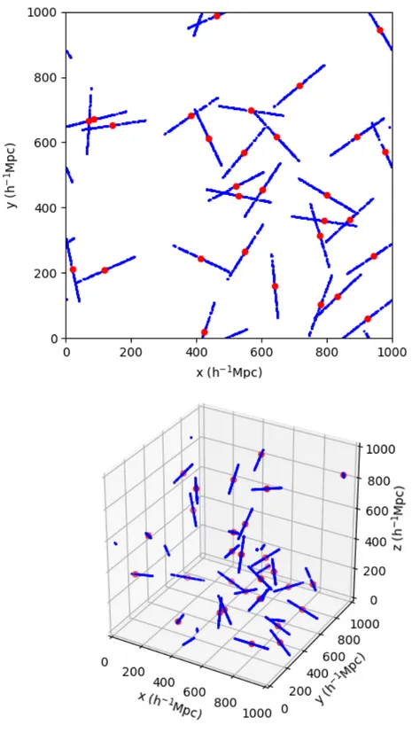
The first Neyman-Scott process to look at is the isotropic segment Cox process (Stoyan et al., 1995). This point process is used for Euclid pipeline validation, and was the first to be extended to provide known non-zero higher multipoles. Stoyan et al. (1995) provides a result for the two point correlation function monopole for this process but no derivation is included, so it is written out here for completeness. The isotropic segment Cox process sets the cluster profile as lines of fixed length Lwith random direction. Figure 2.1 visualises this process in the 2D and 3D cases in periodic volumes for 30 lines each of length 200 h−1_{Mpc. The segment Cox process}

(39)

Figure 2.1: Visualisation of the 2D (top panel) and 3D (bottom panel) isotropic segment Cox process for line length of 200 h−1Mpc in periodic volumes of Lbox =

1000 h−1_{Mpc. Red points are the 30 cluster centres and blue point samplings from}

(40)

cluster density probability distribution is given by p(r) = θ(r)θ(L−r)

L , (2.2.22)

with a length of segment L and the heavyside step functionθ(r) defined by

θ(r) =      1, if r ≥0 0, otherwise. (2.2.23)

The K-function for the segment Cox process can then be calculated from equation 2.2.21. The integrals are reduced to one dimension due to the one dimensional nature of the cluster density profile and the integral over the catalogue volume is reduced to an integral over the finite size of a cluster. This gives

K(r) = 4 3πr 3_h_ρ_i₊ Np L2_N c Z L 0 ds Z r −r dr0θ(s+r0)θ(L−s−r0). (2.2.24)

The integral can be solved graphically (see Figure 2.2) to give

K(r) =      4 3πr 3_h_ρ_i₊Np Nc 2r L − r2 L2 if r ≤L 4 3πr 3_h_ρ_i _otherwise_. (2.2.25)

In other than three dimensions the (4/3)πr3_h_ρ_i_{terms will change to the average}

number of points in a randomly placed hypersphere of radius r rather than in a three dimensional sphere, other terms are unchanged. This can then be used along with equation 2.2.12 to give the correlation function in N dimensions. In all cases the correlation function is zero on scales larger than the line length and non-zero below it. In two dimensions,

ξ(r) =      1 πλs 1 rL− 1 L2 if r≤L 0 otherwise, (2.2.26)

where λs is the density of clusters in the volume, in this case in 2D, given by

λs=Nc/V for V the volume containing the catalogue. In three dimensions,

ξ(r) =      1 2πλs 1 r2_L− _rL12 if r ≤L 0 otherwise. (2.2.27)

(41)

Figure 2.2: Graphical solution to the integral given in equation 2.2.24 for the K function of the segment Cox process. The area to integrate lies within all dashed lines. The black and red dashed lines come from the integration limits and the green and blue lines from the step functions in the integrand.

(42)

On small scales this expression acts like a power law that scales as ∼ r−γ with γ = 2. Snethlage et al. (2002) showed how this slope can be changed so that γ <2 through applying random shifts to the point field.

In order to calculate the projected correlation function the monopole result can be expressed in terms of projected component, rp, and line of sight component, π,

as ξ(rp, π) =      1 2πλs 1 (r2 p+π2)L− 1 √ r2 p+π2L2 if r2 p+π2 ≤L2 0 otherwise. (2.2.28)

We can defineπ0 as the value ofπat eachrp for which the correlation function drops

to zero. It is given by π0(rp) =      p L2₋_r2 p if rp ≤L 0 otherwise. (2.2.29)

The projected correlation function using equation 2.1.9 becomes

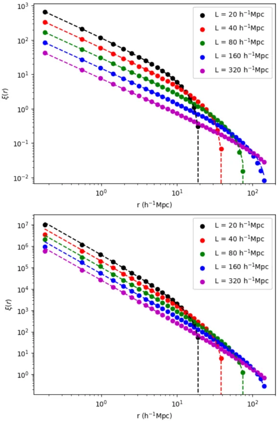
wp(rp) =              2 πλs 1 Lrparctan( πmax rp )− 1 L2 arcsin( πmax rp ) if rp ≤L and πmax ≤π0(rp) 2 πλs 1 Lrparctan( π0(rp) rp )− 1 L2 arcsin( π0(rp) rp ) if rp ≤L and πmax > π0(rp) 0 otherwise. (2.2.30) Verification of the 2D and 3D segment Cox process monopole results are shown in Figure 2.3. In each case 104 lines with an average of 100 points per line are used in a periodic square(2D)/box(3D) with side length 1000 h−1_{Mpc. We generate a}

uniform random catalogue and use the Landay-Szalay estimator (Landy & Szalay, 1993a) for calculating the correlation function as the code used does not support periodic volumes. The number of randoms is set to ten times the number of data points. The number of randoms needs to be sufficient that there are enough random pairs in the smallest bins that the error on the random pair counts in those bins does not impact the final correlation function measurement. In this case we decide that ten times is sufficient based on the good agreement between the measured and theoretical results. For a measurement where the result isn’t predicted beforehand the result can be retested with a new realisation of the same number of randoms

(43)

Figure 2.3: Measurement (dots) and expectation (lines) for the correlation function of the 2D (top panel) and 3D (bottom panel) isotropic segment Cox process for different values of the line length. Details of the test are given in the text.

(44)

Figure 2.4: Ratio of mean of measured correlation function for 1000 Cox process mocks to Cox process theory, calculated by the Euclid 2 point correlation function pipeline for validation purposes. The errors shown correspond to errors on the mean measurement. Plot provided by Viola Allevato.

to assess its robustness. The theoretical prediction lines up well with the measured correlation function for all tested values of the line length at all scales below the line lengths.

Figure 2.4 shows validation of the Euclid 2 point correlation function pipeline using the segment Cox process. The brief mandated that the code was validated to the sub percent level in 200 linear bins between 0 and 200h−1_{Mpc. This plot shows}

this is achieved for all bins except those on the smallest scales. This is because the theoretical function varies quickly over the width of the bin so the approximation that the average value over the bin will equal the theoretical value at the centre of the bin breaks down, and because the theoretical expression is divergent as the separation approaches zero. Integrating the theoretical expression over each bin fixes the small scale discrepancy in all but the first bin, where the pole at zero makes this integration impossible. There is a small but significant disagreement on large scales, where the theoretical result is larger than the estimated one. This bias gets worse as the separation approaches the line length and the correlation function approaches zero. The line length should be set to be significantly larger than the largest relevant separation in order for the estimate to agree well with the theoretical prediction. Here the line length being 2.5 times larger than the largest separation keeps this bias

(45)

below the 1% required accuracy. In order to reach the accuracy shown the mean of 1000 Cox process mocks was calculated. Each of the mocks used 106 _{lines of 500}

h−1_{Mpc with an average of 100 points per line in a 5000} _h−1_{Mpc per side cubic}

box. The large number of points and realisations could be significantly reduced if different scales could be validated with different mocks.

It is worth mentioning the typical amplitude of these Cox process correlation functions. The lower the density of the clusters the higher the amplitude of the correlation function and the higher the signal to noise will be in measuring the correlation function on one cluster/halo scales. The results in figures 2.3 and 2.4 show results for correlation functions with amplitudes far above what is found in the real universe in order that the results have little scatter. The Cox process can produce correlation functions of more realistic amplitudes using higher densities of clusters but the scatter on the final result will be larger.

2.2.2

Thomas process

The Thomas process sets the cluster profile of the Neyman-Scott process to a Gaus-sian (Thomas, 1949). This process is investigated because the two point correlation function in 2D and 3D for an isotropic Gaussian is known from the literature (Stoyan et al., 1995; Moller & Waagepetersen, 2004). This point process is visualised in Fig-ure 2.5 in the 2D case in a periodic box with 30 clusters, each with Gaussian standard deviation of 30 h−1_{Mpc. The cluster centres are the same as the 2D case in figure}

2.1 but the clusters are now theoretically of infinite extent.

In 2 dimensions, for a Gaussian cluster profile with standard deviation σ, the cluster density is ρc(r) = Np Nc s 1 (2πσ2₎2exp −r2 2σ2 , (2.2.31)

and the corresponding correlation function is

ξ(r) = 1 λs s 1 (4πσ2₎2 exp −r2 4σ2 , (2.2.32)

(46)

Figure 2.5: Visualisation of the 2D isotropic Thomas process for 30 Gaussian clusters with σ = 30 h−1_{Mpc and an average of 30 points per cluster in a periodic box of}

side length 1000 h−1Mpc. Red points show cluster centres and blue points show samplings from the point process.

(47)

by ρc(r) = Np Nc s 1 (2πσ2₎3exp −r2 2σ2 , (2.2.33)

which gives a correlation function of ξ(r) = 1 λs s 1 (4πσ2₎3 exp −r2 4σ2 . (2.2.34)

The derivations of these results are special cases of the generalised Thomas pro-cess derivation that will be given in section 2.3.2. Verification of the 2D and 3D Thomas process results are shown in Figure 2.6. 104 _{clusters with an average of 100}

points per cluster are used in a periodic square(2D)/box(3D) with side length 1000 h−1_{Mpc. The number of randoms is set to ten times the number of data points. The}

theoretical prediction lines up well with the measured correlation function below∼

5σ for all cluster sizes tested. The open circles in the plot represent where the value of ξ(r) falls below 10−2 and does not match well with the expectation. Beyond ∼

5σ, the correlation function moves rapidly toward zero and there are too few two-halo pairs in this low cluster density catalogue to accurately approximate such a low amplitude correlation function. The density of clusters could be increased to combat this, but the scatter in one cluster regime would increase.

2.2.3

Other examples from the literature

The Matern process is included here for completeness as it is a common result from the literature (Stoyan et al., 1995). Unlike the segment Cox process and the Thomas process this point process will not be extended to produce a known anisotropy. The Matern process is a point process in which the cluster profile is given by a sphere with uniform density. The cluster density probability distribution for a cluster of radius R with centres_c is given by

p(s) = 3θ(R− |s−sc|)

4πR3 . (2.2.35)

This point process is visualised for 30 clusters of radius 30 h−1_{Mpc in a periodic}

volume in Figure 2.7. The cluster centres are shared with the 2D example in Figure 2.1 and with Figure 2.5. Compared to the Thomas process clusters shown in Figure 2.5 the clusters now have a finite extent.

(48)

Figure 2.6: Measurement (dots) and expecta