Novel Optimization Technique for PI Controller Parameters of
ac/dc PWM Converter using Genetic Algorithms
V M Mishra*, A N Tiwari**, N. K. Sharma***
*G.B.Pant Engg. College, Pauri- Garhwal,( Uttrakhand, India),** M.M.M.Engg. College, Gorakhpur (U.P., India), *** KIET, Ghaziabad (U.P., India)
Address: G B Pant Engg College, Pauri-Garhwal, tel/fax institute 91-1368-228062 E mail:[email protected],[email protected],[email protected]
Article Info ABSTRACT
Article history: Received Nov 9th, 2011 Revised Mar 29th, 2012 Accepted Apr 11th, 2012
The aim of this paper is to present a novel control scheme and designing of reactance parameter of PWM convereter and find the optimized value of parameters for voltage PI controller. Paper describes the application of Genetic Algorithms for optimization of controller parameters of PWM converter. The behavior of the stability region is plotted with different sampling periods.Genetic Algorithms used for off-line searching using the MATLAB, the simulation model of the dc- link PWM ac/dc converter is built up. According to the simulation results, it is known that, the presented control strategy is feasible and valid, and the converter can work well under PMDC motor load condition.
Keyword:
Genetic Algorithms PI voltage controller PWM rectifier THD
Copyright © 2012 Institute of Advanced Engineering and Science. All rights reserved. Corresponding Author:
A N Tiwari,
Departement of Electrical Engineering, M M M Engineering College,
Gorakhpur, Uttar pradesh, India. Email: [email protected]
1. INTRODUCTION
Due to non-linear nature of the converter operation and non-linear nature of the drive load, analysis and controller design of the PWM converter is challenging. The PWM rectifier permits power flow from ac to dc link, in case the load is drawing power and, from dc link to ac source, in case the load is generating power. For the four-quadrant drive control the PWM rectifier is used as front-end converter. During the drive operation, the dc link capacitor voltage is kept constant and ripples free. The three-phase input currents are maintained sinusoidal and in phase with the supply voltages [1, 2, 9, 12].
The PWM rectifier controls the harmonics injected in to the supply system and ensures unity power factor operation. The source inductors provide a power transfer link between two three-phase ac systems i.e., (i) three-phase ac supply and (ii) three phase ac regenerative/back emfs of the PWM rectifier [3, 6, 8].
GA is very different from most of the traditional optimization method. It needs design space to be converted in to genetic space. So, genetic algorithms work with a coding of variables. The advantage of working with a coding of variable space is that, coding discretizes the search space even though the function may continuous. A most important difference between genetic algorithms and most of the traditional optimization methods is that GA uses a population of points at one time in contrast to the single point approach by a traditional optimization methods, transition rules are used they are deterministic in nature but GA uses randomized operators. Random operators improve the search space in an adaptive manner [5, 13].
Each chromosomes of the population are decoded for KP and KI. PWM model including hysteresis
current controller, is simulated on MATLAB, with each value of chromosome (KP and KI). There is one
fitness value corresponding to each chromosome in the population. Each fitness value is divided by the summed up fitness value to obtain fitness ratio (FR) corresponding to each chromosome. Scaled fitness
scaled fitness ratio (SFR) corresponding to each chromosome. A cumulative SFR is assigned to each chromosome by cumulative addition of the corresponding SFRs. The cumulative SFRs lie between 0 and 1. The process of reproduction, crossover and mutation is repeated for many generations till an optimum solution is reached [4, 13]
2. PROPOSED PWM CONVERTER MODEL AND CONTROLLER SCHEMES
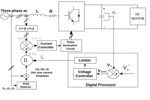
The schematic diagram of proposed high power factor three-phase PWM boost converter is shown in figure 1. The PWM converter permits power flow from ac to dc link in motoring operation and from dc link to ac source during generating operation mode of the dc motor. During the drive operation the dc link capacitor voltage is kept constant and ripples free. The three-phase input currents are maintained sinusoidal and in phase with supply voltages. The converter controls the harmonics injected to the supply system and ensures unity power factor operation. The source inductors provide a power transfer link between two three-phase ac systems i.e., (i) three-three-phase ac supply and (ii) three three-phase ac regenerative/back emfs of the PWM converter. The converter is operated with outer dc link voltage control loop and inner hysteresis current control loop actions. The dc link voltage is sensed and it is subtracted from the reference voltage. The dc link capacitor filters out the ripples present in the dc link voltage. Larger ripples present in the dc link current drawn by the drive inverter, produces larger dc link voltage ripples; hence, appropriately large value of the dc link capacitor is chosen to minimize the ripples. The reference voltage is kept equal the line voltage rating of the PMDC motor. Actual voltage is subtracted from the reference voltage and error is send to PI controller. The output of the PI controller is peak value of reference current. To avoid the reference current amplitude more than the current rating of the converter, a limiter is applied. The limiter limits the peak value of reference currents between a maximum and minimum set values [10, 11, 14, 16].
Hysteresis current controllers are used to control the PWM converter three-phase input currents. The peak amplitude of the reference current is multiplied with three unit vectors. The three unit vectors are generated using three-phase supply voltages obtained from the common coupling point. The three-phase supply voltage templates are divided by their peak amplitudes resulting in Ua, Ub and Uc three unit vectors in phase with
phase ‘a’, phase ‘b’ and phase ‘c’, voltages respectively. These unit vectors are multiplied with peak value of the reference current (obtained from the voltage controller) to give out three phase reference currents. Phase ‘a’ and phase ‘b’ currents are sensed and phase ‘c’ current is produced as negative sum of the two phase sensed currents. Actual currents are subtracted from the respective phase reference currents rendering the three current errors. Using the three current errors I*a_err , I
*
b_err and I *
c_err the hysteresis current controllers generate switching pulses for upper and lower IGBTs of phase ‘a’, phase ‘b’ and phase ‘c’ legs respectively. With voltage and current controllers, the dc link voltage is maintained constant and input three phase current is made sinusoidal and in phase with respective supply phase voltages[5,9,10].
Figure 1. Control scheme of PWM converter.
Current Controller DC MOTOR + -Ua, Ub, Uc Unit sine current
templates Vc L R + -∏ Three-phase ac ic=-(ia+ib) Pulse Generation Circuit Peak Detector Voltage Controller Vc + Verror -Limiter Digital Processor ea,eb,ec c I∗ b I∗ a I∗ a I b I c
I Ia_errIb_errIc_err
* c
V
* m I3. OPTIMIZATION OF PI GAINS USING GENETIC ALGORITHMS
GA works on natural evolution process. The evolution process is operated on chromosomes. The decoded
structures uses of the chromosome are responsible for the performance and natural selection is linked with the performance. In natural selection, the chromosomes having structure which provide desirable performance are reproduced more often than those that having undesirable performance. This natural evolution process is appropriately incorporated in computer algorithms to solve difficult search problems.The aim of the GA is to solve the problem of maximization (or minimization) to be stated in the form of an objective function.
3.1. Generation of Initial Population
The population size is the number of chromosomes in the population. Random bits are generated 21 times (equal to the length of chromosome) and one chromosome (string) is formed. The chromosome is decoded for KP and KI and tested whether it is within the OKP4KI4O region of Figure 3 or not. If KP and KI
are within the OKP4KI4O region the chromosome is accepted otherwise rejected. Total numbers of acceptable
chromosomes generated are equal to the population size. For population size is 20 and the randomly generated chromosomes for initial or first population are shown in Figure 4.
3.2. Objective Function and Fitness Value
Each chromosomes of the population are decoded for KP and KI. PWM model including hysteresis
current controller is simulated on MATLAB, with each value of chromosome (KP and KI). The performance
of controller gains is judged by value of ITAE (Integral Time Absolute Error). The performance index ITAE is chosen as objective function. Fitness function is defined as 1/ (IATE+1). If more than 5% overshoot occurs in starting voltage response a 75% of the penalty is imposed to the fitness value. There is one fitness value corresponding to each chromosome in the population.
3.3. Reproduction (Using Roulette Wheel Selection Criteria)
Each fitness value is divided by the summed up fitness value to obtain fitness ratio (FR) corresponding to each chromosome. The fitness values corresponding to each chromosome in the population are scaled as (FR-min.FR)/(max. FR – min. FR). Where, min.FR and max.FR are minimum and maximum values of fitness ratios obtained from the fitness values of the chromosomes in the population. Scaled fitness values are summed up. Each scaled fitness value is divided by the summed up scaled fitness value to obtain scaled fitness ratio (SFR) corresponding to each chromosome. A cumulative SFR is assigned to each chromosome by cumulative addition of the corresponding SFRs. The cumulative SFRs lie between 0 and 1. Random numbers between 0 and 1 are generated 20 (population size) times. If the magnitude of generated random number is equal or immediate below to cumulative SFR of a chromosome in the population, the chromosome is copied to new population. Total 20 times (equal to population size) chromosomes are copied. The probability of generating a random number is uniform throughout between 0 and 1, hence, probability of selection of more number of copies is high for the chromosome having high fitness value.
3.4. Crossover and Mutation
Crossover probability is chosen 70%. Out of 20 chromosomes, first 7 chromosomes are randomly chosen in one group and out of remaining 13 chromosomes, another 7 chromosomes are randomly chosen in other group, the third group stores remaining 6 chromosomes. A random number is generated from 1 to 21(length of bits in chromosome), this number is taken as crossover site. First chromosomes of first group and second group are picked up and bits of their chromosomes beyond the crossover site are exchanged. Another random crossover site is generated and second chromosomes of first group and second group are picked up and bits of their chromosomes after the crossover site are exchanged. Similar process is repeated for all the 7 chromosomes of the first and second groups are crossover. A new population is obtained by combining the 14 chromosomes of crossover groups and 6 chromosomes of the third group. Mutation probability is chosen 0.5%. In the new population total 0.5% string elements are altered randomly.
Chromosomes of the new population are decoded for KP and KI, and any chromosomes found lying
outside of the region OKP4KI4O of Figure 4 are replaced by a randomly generated new chromosome lying
inside the region OKP4KI4O. Now, the process of reproduction, crossover and mutation is repeated for many
generations till an optimum solution is reached. The population size, crossover probability, mutation probability and number of generations can be varied for repeated search to optimise the solution.
3.5. Optimum Gains using GA
The GAs is run for off line optimisation of the controller gains for the population size=20, crossover probability=70%, mutation probability=0.5% till 25 generations. The fitness values for 1st and 25th generation are shown in figure 7 and chromosomes for 1st and 25th generation are plotted in figure 5 shows the best values of chromosomes after 25th generation. The best pair of controller gain obtained as KP=0.6021 and
KI=0.1056.
4. CONTROLLER DESIGN FOR THE PWM CONVERTER
The control strategy of PWM Converter regulates input current and output dc link voltage. The control analysis of the converter can be simplified by making minor (inner) current loop independent of the outer voltage loop. The only way to delink the inner current loop with outer loop is to make the inner loop much faster than the outer loop. The inner current loop can be made faster by keeping high ratio of the dc bus voltage to the value of the phase voltage and/or by reducing the value of source inductor and/or by improving the gain parameters of the current loop controller. The current control scheme opted is hysteresis current controller as shown in Fig 1, which makes the input line currents in phase with their respective utility phase voltages. At steady-state operation of the converter, the switching pattern generated by the current controller is fixed for one cycle of the utility supply frequency. Hence, the average voltage generated due to PWM ramp switching is also a sinusoidal EMF [15].
The hysteresis current controller is in inner loop and it operates in stationary reference frame.The space vector current equation is represented as
s i
E =R I+L I s+E (1)
Input line currents, supply phase voltages and regenerative emfs are represented by space vector (Using Park’s Transformation) as below
2 2 j j j 0 3 3 a b c
2
I
i e
i e
i e
3
π π −
=
+
+
; 2 2 j j j 0 3 3 s an bn cn2
E
e e
e e
e e
3
π π −
=
+
+
and 2 2 j j j 0 3 3 i An Bn Cn2
E
e e
e e
e e
3
π π −
=
+
+
.Power balance concept is applied for design of outer voltage control loop. The power balance equation of the PWM Converter is 2 2 C 2 2 C s L V d 1 3 d 1 CV E I I R LI dt 2 R 2 dt 2 + = − − (2) The overall aim of the controller is to control input line current and output dc link voltage. Hence, at steady-state operating point of dc link voltage (Vco) and input current (Io), the equation (2) can be written as
2 2 C o s o o L V 3 E I I R R 2 = − (3)
Choosing smaller value of the line current from equation (3), the line current space vector (Io) is,
2 2 s s co o L E E 8V 1 I 2 R R 3RR = − − (4)
Imposing small disturbance around the operating point, i.e., replacing the dc link voltage with (Vco+∆Vc) and
line current with (Io+∆I), the dynamic equation of the system represented by equation (2) is obtained and
neglecting square terms of ∆Vc and ∆I and simplifying it, we get
( ) ( o o S) L S o c co L LI s 1 2I R E R E R I V I V R C s 1 + − − ∆ = ∆ + 3 2 4 2 (5)
The above dynamic equation of the voltage transfer function can be written as
( )
(
(
nv)
)
v v v T s 1 G s A T s 1 + = + (6)Where
(
)
(
)
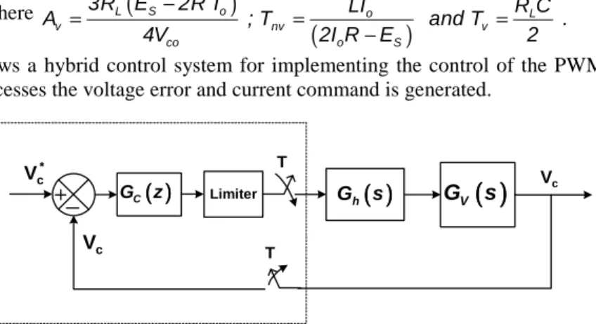
L S o o L v nv v co o S 3R E 2R I LI R C A ; T and T . 4V 2I R E 2 − = = = −Figure 2 shows a hybrid control system for implementing the control of the PWM converter. The voltage controller processes the voltage error and current command is generated.
Figure 2. Closed loop control system of dc link voltage controller
The limiter is replaced with Describing Function in order to linearize the saturation non-linearity. It is observed that the describing function of the saturation non-linearity is only amplitude dependent. Hence, it is frequency invariant having zero phase shift. For stability analysis purpose the limiter block is omitted. The block Gh(s) is transfer function of Zero Order Hold. It is given as
(
sT)
h e G ( s ) s − − = 1 (7)Controller gain function is given as
(
)
(
)
PV IV C K z 1 K z G ( z ) z 1 − + = − (8)Closed loop transfer function of the overall voltage control system is,
( )
( )
z D z N ) z ( G G ) z ( G 1 ) z ( G G ) z ( G ) z ( V ) z ( V ) z ( G Z Z V h C V h C * C C o = + = = (9)The z-transform of numerator of equation (9) is written as
(
)
(
)
( )
(
)
nv v PV IV v Z v T z 1 T (1 ) z-1 K K Z A N ( z ) T z z 1 α α − + − + = − − (10) Where,e
TV T-=
α
.The characteristic equation of the system is
( )
z
1
N
( )
z
0
D
z=
+
z=
(11)Substituting equation (11) into equations (9) and after simplification; the closed loop transfer function is written as
( ) (
)
{
1 v(
)
} (
0 v)
2 2 v 0 1 2 2 oT
N
z
1
T
N
z
N
T
N
z
N
z
N
z
G
α
α
+
+
+
−
+
+
+
+
=
(12)(
)
(
)(
)
(
)
2 v nv PV IV 1 v v PV IV V nv PV IV 0 v PV nv v PV v Where, N A T K K , N A T 1 K K A T 2K K and N A K T A K T (1 );α
α
= + = − + − + = − −From equation (12), the characteristic equation is
(
T
N
)
z
{
N
1T
v(
1
)
} (
z
N
0T
v)
0
22
v
+
+
−
+
α
+
+
α
=
(13)For stability analysis of the system, Bilinear transformation i.e., z= (1+r)/(1-r) = ejθr is applied with equation (13). According to Bilinear transformation, on unit circle in the z-plane, varying θr anticlockwise from –π through 0 to +π, ωr varies from -∞ through 0 to +∞ in r-plane, where r=jωr . The left half r-plane maps the interior of the unit circle in the z-r-plane. Substituting z=(1+r)/(1- r) in the characteristic equation (13), we get,
(
)
{
(
)
}
(
)
{
(
) (
)
}
(
)
(
(
)
)
(
)
{
}
2 v 2 1 v 0 v v 2 0 v T N N T 1 N T r 2 T N N T r T N N T 1 N T 0 α α α α α + − − + + + + + − + + + + − + + + = Limiter(((( ))))
C G z Gh(((( ))))
sDIGITAL SYSYTEM ANALOG SYSYTEM
c V * c V
(((( ))))
V G s Vc T TThe roots of second order characteristic equation are always in the left half of r-plane if all coefficients are positive. Hence, three conditions are deduced corresponding to each coefficient of the characteristic equation to be greater than zero.
Condition – I:
(
)
{
(
)
} (
)
[
Tv +N2 − N1−Tv 1+α + N0 +αTv]
>0 Substituting values of N2, N1, N0, and simplifying, we get(
)
{
}
{
(
)
}
(
)
pV v nv v v IV v nv v v v 2K 2 A T A T 1α
K 2 A T A T 1α
2T 1α
0 − − + − − + + > (15)The term
{
T
v(
1
+α
)
}
>
0
for converter operation, dividing by positive quantity2
T
v(
1
+
α
)
on both sides of the equation (15) and solving, we havePV IV P1 I1
K
K
1
K
K
+
<
(16) Where,(
)
(
)
{
v v v nv}
v 1 P AT 1 2AT 1 T K = +α −α − and KI1=2KP1. Condition – II:(
) (
)
{
Tv +N2 − N0 +α
Tv}
>0 Substituting values of N2, N1 and simplifying, we get(
)
{
}
(
)
(
)
pV v v IV v nv v K A T 1 α K A T T 1 α 0 − + + − > (17)Since,
T
v(
1
−
α
)
is always positive for the converter, hence, dividing byT
v(
1
−
α
)
on both sides of inequality (17), we get PV IV P 2 I 2 K K 1 K K + < (18) Where,(
)
− − = − = nv v v I2 v 2 P T A 1 T K and A 1 Kα
. Condition –III:(
)
(
(
)
) (
)
{
Tv +N2 + N1 −Tv 1+α
+ N0 +α
Tv}
>0 Substituting values of N2, N1 & N0, and simplifying, we have(
1
)
K
0
T
A
v v−
α
I>
(19)Placing values of Av, Tv and
α
, we write(
)
v T 2 T L IV s o co 3R C K E 2I R 1 e 0 8V − − − > (20) Polarity of Vco and gain KIV are always kept positive. Hence, to satisfy the stability condition, the two termsin braces are required to be either positive or both negative. The first term in braces is (Es-2IoR)>0 for the converter. The second term in braces is (1-e(-T/Tv))>0 when RL is positive i.e., for converter operation.
Hence, the inequality represented by equation (20) is always satisfied for KI>0.
The parameters of the PWM converter are chosen as, VCo=590 Volts, Es=230 Volts, L=4.90 mH,
R=2.5 Ω, RL=50 Ω, C=5050 µF and sampling period T=0.4 ms. The steady-state current (Io) is obtained from
equation (4), for the given parameters. The calculated value of Io is 11.54 amp for the converter. If sampling
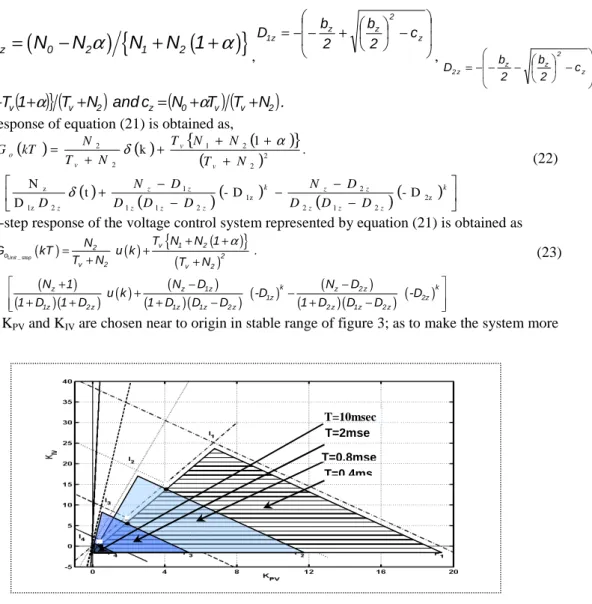
period T is increased, the stability region shrinks. Figure 3 shows stability regions for sampling periods 0.4m sec, 0.8m sec, 2m sec and 10m sec as OP1I1O, OP2I2O, OP3I3O, and OP4I4O respectively.
Equation (12) is simplified and written as
( )
{
(
(
)
)
}
(
(
)(
)
)
+ + + + + + + + = z 2 z 1 z 2 2 v 2 1 v 2 v 2 o D z D z N z N T 1 N N T N T N z Gα
(21)Where,
N
z=
(
N
0−
N
2α
)
{
N
1+
N 1
2(
+
α
)
}
, − + − − = z 2 z z z 1 c 2 b 2 b D , − − − − = z 2 z z z 2 c 2 b 2 b D ,bz={
N1−Tv( )
1+α
} (
Tv+N2)
and cz=(
N0+α
Tv) (
Tv+N2)
. Impulse response of equation (21) is obtained as,( )
( )
{
(
(
)
)
}
( )
(
) (
)
(
) (
)
− − − − − + + + + + + = k z z z z z k z z z z z z v v v o D D D D N D D D D N D N T N N T N T N kT G 2z 2 1 2 2 1z 2 1 1 1 2 1z z 2 2 2 1 2 2 D -D -t D N . 1 k δ α δ (22)Also, unit-step response of the voltage control system represented by equation (21) is obtained as
( )
( )
{
(
(
)
)
}
(
)
(
)(
) ( )
(
(
)(
)
) (
)
(
(
)(
)
) (
)
Unit _ step v 1 2 2 o 2 v 2 v 2 k k z z 1z z 2 z 1z 2z 1z 2 z 1z 1z 2 z 2 z 1z 2 z T N N 1 N G kT u k . T N T N N 1 N D N D u k -D -D 1 D 1 D 1 D D D 1 D D D α + + = + + + + − − + − + + + − + − (23)Values of KPV and KIV are chosen near to origin in stable range of figure 3; as to make the system more
stable.
Figure 3. Variation in stability region with sampling period on KPV and KIV plane
5. RESULT AND ANALYSIS
The gains obtained by trial and error cannot be optimum. To obtain near optimum value of the gains in region OP4CDO of the KPV-KIV plane of figure 3; space search method, based on Genetic Algorithms is
applied. Initially 300 chromosomes [KPV KIV] population is generated. The minimum values of both KPV and
KIV are kept 0.0001 and the maximum values are restricted in the shaded portion of figure 3. The unit step
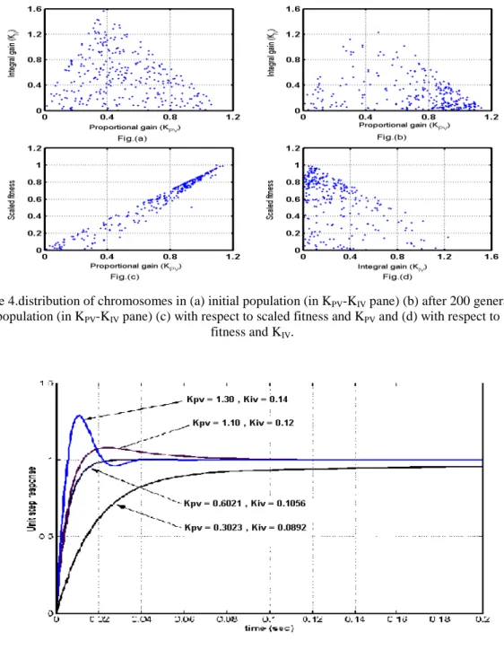
response is observed and integral time absolute error (ITAE) is chosen as objective function. The fitness function is defined as Fitness = (1-0.5 penalty)(100/(1+ITAE)). The value of penalty is chosen 1 if there is an overshoot more than 2%, otherwise the value of penalty is kept zero. A chromosome with higher value of scaled fitness has fair chance to survive and produce off springs in next generations. The process to produce next generation is via reproduction, crossover and mutation. 4(a) is initial population of 300 chromosomes and figure 4(b) is population of the chromosomes after 200 generations. After 200 generations, majority of the chromosomes bear higher values of fitness. The chromosomes shown in figure 4(b) are concentrated at higher value of KPV and lower value of KIV. In figure 4(b) and (c) the chromosomes after 200
generations are plotted with their scaled fitness and decoded values of respective KPV and KIV. The
chromosome having highest scaled fitness decoded as KPV=0.6021 and KIV=0.1056. The step response curves
with different controller gains KPV=1.30 and KIV=0.14, KPV=1.1 and KIV=0.12, KPV=0.6021 and KIV=0.1056,
KPV=0.3023 and KIV=0.0892 are shown in figure 5. The optimised gain KPV=0.6021 and KIV=0.1056 is most
suitable for the voltage controller.
C
B
A
T=10msec T=2mse T=0.8mse T=0.4msFigure 4.distribution of chromosomes in (a) initial population (in KPV-KIV pane) (b) after 200 generations
final population (in KPV-KIV pane) (c) with respect to scaled fitness and KPV and (d) with respect to scaled
fitness and KIV.
Figure 5.Unit step responses with different controller gains.
6. CONCLUSIONS
The closed loop control system is developed based on the converter model. An analysis has been carried out to find the stability region of the voltage controller on KP and KI plane. The unit impulse and unit step responses are derived
for the closed loop voltage controller of the PWM converter. The optimum PI voltage controller gain parameters are obtained using the Genetic algorithms search method. The PWM converter system provides the desired response with the optimized gains.
REFERENCES
[1] Boon Tech Ooi, John C.Salmon et al,”A three Phase controlled- current PWM converter with leading power factor,”IEEE Trans.on Ind. Applns, Vol.IA-23, No.1, pp.78-84, Jan/Feb 1987.
[2] Boon Tech Ooi, Juan W.Dixon et al,” An Intregrated AC drive system using a controlled- current PWM rectifier/Inverter link,” IEEE Trans. On Industrial Electronics, Vol.3, No.`1,pp.64-70, Jan. 1988.
[3] Rusong Wu, S. B. Dewan and G. R. Slemon, “Analysis of a PWM ac to dc Voltage Source Converter Using PWM with Phase and Amplitude control,'' IEEE Trans. on Ind. Applns., Vol. 27, No. 2, pp. 355-364, March/April, 1991. [4] M.O. Eissa, S.B. Leeb, G.C. Verghese and A.M. Stankovic, “Fast controller for a unity-Power-Factor PWM
[5] K.F.Man, K.S.Tang and S.kwong,” Genetic Algorithms: Concepts and application, IEEE Trans. On Ind.
Electronics, vol. 43, no.5, pp.519-533, Oct 1996.
[6] R. Blundell, L. Kupka and S. Spiteri, “AC-DC Converter with Unity Power Factor and Minimum Harmonic Content of Line Current: Design Considerations,'' IEE Proc. Electric Power Applications, Vol. 145, No. 6, pp.553-558, November 1998.
[7] N. Bruyant, M. Machmoum and P. Chevrel “Control of a three-phase active power filter with optimised design of the energy storage capacitor”,in Proc. PESC Conference, Kobe, Japan, vol. 1, pp. 878-883,1998
[8] M.T. Tsai, W.I. Tsai, “Analysis and design of three-phase AC-toDC converters with high power factor and near-optimum feedforward”, IEEETrans. on Ind. Electronics, vol. 46, no. 3, pp 535-543, June 1999.
[9] Ming-Tsung Tsai and W.I.Tsai,”Analysis and Design of Three Phase AC to DC Converters with High Power Factor and Near Optimum Feed Forward,IEEE Trans. Industrial Application,Vol.46,No3,pp.535-543,June 1999. [10] A. N. Tiwari, Pramod Agarwal and S. P. Srivastava, “Analysis and Simulation of PWM Boost Rectifier”,
International conference on Computer Application in Electrical Engineering, (CERA 01) at I.I.T. Roorkee, pp 347-359, Feb. 21-23, 2001.
[11] Bhim Singh, B. P. Singh and Mukesh Kumar, “Power Quality Improvement of AC Mains for Single-Phase Rectifier-Inverter Fed PMBLDC Motor Drive for Air Conditioning,'' Proceedings of the International Conference
on Computer Applications in Electrical Engineering Recent Advances, CERA 01, pp. 371-380, Feb. 21-23, 2002.
[12] A. N. Tiwari, Pramod Agarwal and S. P. Srivastava, “Modified Hysteresis Controlled PWM Rectifier,” IEE Proc.
Electric. Power Applications, Vol. 104, Issue- 4, pp. 389-396, July 2003.
[13] Bimal K. Bose.Modern. Power Electronic and AC Drives, Beijing: Machine Industry Publishing House, 2003. [14] Hongjin Song1*, Xinchun Shi, Guoliang Zhou,” Research On Three Phase Voltage-source PWM Rectifier Based
On Nonlinear Control Strategies,” Proceeding of International Conference on Electrical Machines and Systems,
Oct. 8-11, Seoul, Korea, 2007.
[15] Dunisha Wijeralne and Gerry Moschopous,”Analysis & Design of a Novel Integrated Three Phase Single Stage AC/DC PWM converter,” IEEE 2010.
[16] Wang Jianhna, Zhang Fangha et al,”Modeling and analysis of a Buck/Boost Bidirectional converter with Developed PWM Switch Model,” International conference on Power Electronics ECEE Asia,May30-June
3,2011,The Shilla Jeju, Korea.
BIOGRAPHY OF AUTHORS
Mr. V M Mishra born in India. He received B.E. Degree from MMM Engineering College
Gorakhpur, India in 1988, MTech from Regional Engineering College, Kurushetra, India in 1995, and pursuing Ph.D degree from the UP Technical University Lucknow, India, all in electrical engineering. In 2005 he joined G B Pant Engg College Pauri Garhwal. Before 2005, he was working in MMM Engg College Gorakhpur.His main area of interest includes power electronics control, power quality applications, active power filters, electrical drives and wind energy conversion systems
Dr.A.N Tiwari born in india. He received B.E. Degree from NIT Calicut , India in 1988, MTech
from University of Roorkee (Now it is Indian Institue ofTechnology Roorkee) India in 1994, and the Ph.D degree from the Indian Institute Of Technology Roorkee India in 2003, all in electrical engineering. In 1989 he joined M M M Engg College Gorakhpur. His main area of interest includes power electronics control, power quality applications, active power filters, electrical drives and wind energy conversion systems.
Dr N K Sharma (B, 86 and M, 93) got his B. Sc. Engg. from Faculty of Engg. Dayalbagh
Educational Institute (Deemed Univ.) Agra, M. Tech. and Ph. D. from IIT Kanpur. Presently he is professor in KIET, Ghaziabad, INDIA. He is Member Board of studies (Electrical and Electronics), Mahamaya Technical University, Noida, UP. He have written more than 30 research papers, supervised 5 M. Tech. and supervising 4 Ph.D.s. His area of research includes Power System Restructuring, FACTS, Network Analysis and Synthesis.