Endogenous monetary policy regime change

ENDOGENOUS MONETARY POLICY REGIME CHANGE

Troy Davig and Eric M. Leeper

September 2006

RWP 06-11

Abstract:

This paper makes changes in monetary policy rules (or regimes) endogenous.

Changes are triggered when certain endogenous variables cross specified thresholds.

Rational expectations equilibria are examined in three models of threshold switching to

illustrate that (i) expectations formation effects generated by the possibility of regime

change can be quantitatively important; (ii) symmetric shocks can have asymmetric

effects; (iii) endogenous switching is a natural way to formally model preemptive

policy actions. In a conventional calibrated model, preemptive policy shifts agents’

expectations, enhancing the ability of policy to offset demand shocks; this yields a

quantitatively significant “preemption dividend.”

Keywords

: Threshold switching, Taylor rule, asymmetry, preemptive policy

JEL classification

: E31, E32, E52, E58

Date

: July 14, 2006. Prepared for the NBER International Seminar on Macroeconomics

meeting in Tallinn, Estonia, June 16-17, 2006. Research Department, Federal Reserve

Bank of Kansas City, Troy.Davig@kc.frb.org; Department of Economics, Indiana

University and NBER, eleeper@indiana.edu. We thank Rich Clarida, Jeff Frankel,

Jesper Lind´e, Lucrezia Reichlin, Ken West, and conference participants for helpful

suggestions. Leeper acknowledges support from NSF Grant SES-0452599. The views

expressed herein are solely those of the authors and do not necessarily reflect the views

of the Federal Reserve Bank of Kansas City or the Federal Reserve System.

1.

Introduction

Perhaps the most important advance in the monetary policy literature over the past

20 years is the explicit recognition that policy behavior is purposeful and responds

endogenously to the state of the economy. Substantial progress has been made by

research that examines how various monetary policy rules perform in dynamic

sto-chastic general equilibrium (DSGE) models. A prominent example of such a rule is

Taylor’s (1993) rule, which has the central bank adjust the short-term nominal

inter-est rate in response to fluctuations in inflation and some measure of output. Rare is

the paper now that posits an exogenous process for money growth and claims to offer

practical policy advice.

A substantial line of empirical work finds that Taylor’s or other simple rules

de-scribing purposeful behavior display important time variation in the United States

[Clarida, Gali, and Gertler (2000), Lubik and Schorfheide (2004), Favero and

Mona-celli (2005), Sims and Zha (2006)]. Although particulars vary, a common theme across

much of the empirical work on time variation in policy behavior is that changes in

policy behavior are exogenous. Recent work embeds Markov switching processes for

policy in DSGE models to interpret these empirical findings [Davig, Leeper, and

Chung (2004), Davig and Leeper (2006a,b)].

Because both the empirical and theoretical work on regime change treat the changes

as exogenous, in an important sense the work is inconsistent with a central tenet

underlying the Taylor rule: monetary policy behavior is purposeful and reacts

sys-tematically to changes in the macroeconomic environment. This paper makes regime

change endogenous, taking a step toward resolving this inconsistency.

We distinguish two types of effects from exogenous disturbances.

Direct effects

are the usual impacts of shocks that arise when agents place zero probability on

regime change, corresponding to a fixed-regime setup.

Expectations formation effects

arise whenever agents’ rational expectations of future regime change induce them to

alter their expectations functions. Expectations formation effects are the difference

between the impact of a shock when regime can change and the impact when regime

is forever fixed.

The paper shows that even very simple threshold-style methods for endogenizing

regime changes can generate rich dynamics. The rich dynamics allow models that are

linear, except for policy behavior, to display three features that connect to theoretical

1_{There is also work that assumes that policy behavior switches exogenously among different}

exogenous rules for the evolution of policy variables [for example, Andolfatto and Gomme (2003), Leeper and Zha (2003), Davig (2004), and Owyang and Ramey (2004)].

2_{Some work examines one-time, permanent endogenous regime changes [for example, Sims (1997),}

Daniel (2003), and Mackowiak (2006)].

and empirical work on the impacts of shocks and to observations about how central

banks act:

(1) Expectations formation effects generated by the possibility of regime change

can be quantitatively important.

(2) Symmetric policy shocks can produce asymmetric effects.

(3) Preemptive policy behavior enhances the effectiveness of policy actions and

delivers a quantitatively significant “preemption dividend.”

Endogenous switching shares the feature of quantitatively important expectations

formation effects with exogenous switching. Davig and Leeper (2006b) emphasize that

if monetary policy switches exogenously between a more-active and a less-active

reac-tion against inflareac-tion, agents’ expectareac-tions and, therefore, the equilibrium outcomes

always reflect the possibility that regime can change in the future. For example,

ex-pectations of a more-active policy regime in the future diminish the impacts of shocks

on current inflation, even when the current regime is less active.

Features (2) and (3) emerge with threshold endogenous switching, but are absent

when regimes switch exogenously.

The second feature connects to a growing body of empirical evidence suggests that

typical macroeconomic shocks—such as oil prices, government spending, or nominal

aggregate demand—have nonlinear effects on the economy [for example, DeLong and

Summers (1988), Cover (1992), Hooker and Knetter (1996), Hooker (2002), Ravn and

Sola (2004), Choi and Devereux (2005), Cologni and Manera (2006)]. Some

asym-metric effects have been attributed to nonlinearities in the structure of the economy,

such as real and nominal rigidities or changes in availability of financing over the

busi-ness cycle [for example, Akerlof and Yellen (1985), Ball and Romer (1990), Ball and

Mankiw (1994), Bernanke and Gertler (1989, 1995), Gertler (1992)]. Surico (2003,

2006) estimates central bank preferences and finds evidence of asymmetric loss

func-tions at the Federal Reserve, at the European Central Bank, and, prior to monetary

union, at the Bundesbank. Asymmetric policy preferences also underlie the

“oppor-tunistic disinflation” argument of Orphanides and Wilcox (2002). In this paper, all

asymmetries arise from nonlinearities in the monetary policy process. Nonlinearities

stem from discrete shifts in policy rules that are triggered by changes in the state of

the economy.

The third feature arises from the emphasis central bankers place on the intrinsic

forward-looking nature of monetary policymaking [Bernanke (2004)]. Because of lags

in when monetary policy actions affect real activity and inflation, central banks need

to act before economic conditions deteriorate. A famous instance of forward-looking

policy occurred in 1994 when the Federal Reserve moved preemptively against

in-creases in inflation that had only begun to show up in long-term bond yields.

Good-friend (2005) concludes that the preemptive strike was successful, as inflation

re-mained low and long rates declined. Preemptive actions of this sort, while playing a

central role in central bank thinking, have not been extensively modeled.

The paper applies a simple framework to implement endogenous monetary policy

regime switching. When the central bank’s target variables cross specified thresholds,

the policy rule changes. One policy process that we use posits that if at date

t

−

1

inflation is less than some threshold,

π

,

policy obeys a usual Taylor rule at

t

; if

inflation equals or exceeds

π

,

the central bank implements a more aggressive stance

at

t

.

On the surface, this setup may seem deterministic: given current inflation, next

period’s regime is known exactly. But threshold switching makes forming rational

expectations of regimes two or more periods in the future nontrivial, as they depend

on the joint distribution of all the exogenous disturbances and on the structure of

the economy. Because expectations of all future regimes are updated each period to

incorporate news about realizations of shocks, threshold switching is a special case of

a Markov process with endogenous time-varying probabilities.

The examples of endogenous switching that we present connect well to the behavior

of inflation targeting central banks.

Strict inflation targeting, which is far more

prominent in academic discussions than in actual central banking, lines up with a

threshold inflation rate,

π

,

that triggers shifts in the policy rule. Flexible inflation

targeting, which many central banks claim to pursue, involves more complex triggers

that depend on both the threshold inflation rate and some measure of the output gap.

As applied to inflation targeting, endogenous switching departs from the usual

linear-quadratic framework by embedding the notion that the central bank has

asym-metric preferences over its objectives, a possibility that Blinder (1997) discusses. If

central bankers would prefer to be 25 basis points below their inflation target than

above it, this can create a left-skewed distribution of equilibrium inflation.

This paper fits firmly into the literature that studies how DSGE models perform

under various

ad hoc

policy rules, such as Taylor rules. That literature adopts the

perspective that policy seeks second-best rules, rather than optimal rules, perhaps

because the underlying exogenous shocks are not observed and uncertainty about the

economy prevents them from being accurately inferred from observable time series.

Second-best rules make policy choices a function of observables, like inflation and

output, which the central bank aims to target.

Section 2 briefly compares various specifications of monetary policy— fixed-regime,

exogenous switching, and endogenous switching. Threshold switching in a

flexible-price model of inflation determination is used in sections 3 and 4 to illustrate the

expectations formation effects and asymmetric distributions that endogenous

switch-ing generates. Section 4 details how agents form rational expectations, developswitch-ing a

time-varying probabilities interpretation of regime change. Section 5 embeds

thresh-old switching in the workhorse new Keynesian model and displays the impacts of

aggregate supply shocks on inflation and output dynamics. The implications of a

more plausible characterization of monetary policy behavior—in which both inflation

and output thresholds determine the policy rule—are also laid out. Section 6

com-bines a dynamic threshold— involving past, current, and expected inflation—with a

hybrid new Keynesian model to show how central banks might preemptively strike

against inflation. In a calibrated version of the model, preemptive policy behavior

is shown to enhance the effectiveness of policy actions, delivering a quantitatively

significant “preemption dividend.” Section 7 concludes.

2.

Quick Overview of Endogenous Regime Change

Monetary policy rules, such as Taylor’s, are state-contingent in the sense that

the policy interest rate adjusts to the state of the economy, where a fixed set of

parameters govern the degree of adjustment. In an environment with endogenous

regime-switching, the policy rule is state-contingent in this conventional sense, but

also in a broader sense. Namely, the parameters governing the degree of adjustment

of the interest rate to economic variables are themselves a function of the economic

state. For example, high rates of inflation may be particularly alarming to policy

makers and trigger a systematically more aggressive response to inflation than in

states with more benign rates of inflation.

To understand endogenous switching, it is useful to review fixed-regime and

ex-ogenous switching specifications of policy behavior. Consider the simplified Taylor

rule

i

=

κ

+

απ

+

ε

,

(1)

where

i

is the short-term nominal interest rate controlled by the central bank,

π

is

the inflation rate, and

ε

∼

i.i.d. N

(0

, σ

) is an exogenous policy disturbance. This

rule is state-contingent in the sense that the nominal interest rate adjusts to the

inflation rate, which itself is a function of the underlying state vector describing the

economy. However, the systematic component of policy,

α,

is constant. All deviations

of

i

from

κ

+

απ

are folded into the exogenous shock.

An exogenously switching rule extends this framework to

where

S

is a discrete-valued random variable that evolves stochastically and

inde-pendently of the endogenous economic variables. Now monetary policy is a set of

different rules of the form in (1), with a stochastic process governing the dynamic

evolution of the rules. This makes the policy

rule

rather than just the policy

instru-ment (the interest rate) state-contingent. In both (1) and (2), the parameters

κ

and

α

are given exogenously. The key difference between the two specifications is that

(2) introduces a new source of disturbance to the economy, the process governing

S

,

with important implications for expectations formation.

A simple example of endogenous switching makes the parameters of the monetary

policy rule functions of lagged endogenous variables, as in

i

=

κ

(

π

) +

α

(

π

)

π

+

ε

,

(3)

where the monetary rule again is state-contingent, except that the state is now a

lagged endogenous variable. In principle,

κ

(

·

) and

α

(

·

)

,

to be step functions. As

implemented in this paper, endogenous switching can make the functions

κ

(

·

) and

α

(

·

) either deterministic or stochastic functions of

π

.

Evidently, there is no sharp conceptual distinction between endogenous “regime

change” and nonlinear policy rules. The former is a discrete approximation to the

latter. Discreteness may have some practical advantages to a central bank that seeks

to communicate clearly about its policy actions: it is far easier to inform the public

about two distinct policy stances—“normal” and “tight,” for instance—than about

the continuum of responses implied by a response to inflation that is a continuous

function of the inflation rate. Discreteness also serves a pedagogical purpose: it lends

itself to sharper interpretations of the resulting equilibria.

3.

The Monetary Policy Process

We assume a monetary policy process that permits the monetary authority to vary

its response to contemporaneous inflation depending on the state of the economy. For

example, a monetary authority may respond systematically more aggressively when

inflation exceeds a particular threshold and less aggressively when inflation is below

the threshold.

When the threshold depends on lagged inflation, the monetary authority sets the

nominal interest rate using the rule

i

=

α

π

+

γ

x

,

(4)

5_{The phrase “respond systematically more aggressively” may seem redundant. We use it to} emphasize that the central bank isnot raising the nominal interest rate because of the realization of an additive shock. Instead, it is changing the function that maps economic conditions into policy choices.

where

x

is a measure of the output gap. The coefficients on inflation and the output

gap are functions of the inflation threshold,

π

,

and lagged inflation,

α

= (1

−

I

[

π

≥

π

])

α

+

I

[

π

≥

π

]

α

,

(5)

γ

= (1

−

I

[

π

≥

π

])

γ

+

I

[

π

≥

π

]

γ

,

(6)

where

I

[

·

] is the indicator function.

In sections 5 and 6, we consider more

sophisti-cated specifications that incorporate the output gap into the threshold and thresholds

that depend on expected inflation. In all cases, the monetary policy process

incor-porates a state-contingent systematic component of policy, so the interest rate rule

used to implement policy varies with economic conditions. This represents the point

of departure from simple instrument rules in which the systematic response of policy

is invariant across time and states.

4.

A Fisherian Model of Inflation

A simple model of inflation determination combines a standard Fisher equation

with an interest rate rule for monetary policy. The Fisher equation can be derived

from a perfectly competitive endowment economy with flexible prices and a one-period

nominal bond. A linearized asset-pricing equation for the nominal bond is given by

i

=

E

π

+

E

r

,

(7)

where

r

denotes the real rate at

t

. The real rate evolves exogenously according to

r

=

ρr

+

υ

,

(8)

where 0

≤

ρ <

1 and

υ

is an

i.i.d.

random variable with a doubly truncated normal

distribution with mean of 0, variance of

σ

, and symmetric truncation points. In

the special fixed-regime case where

α

=

α

=

α >

1 in (5), equilibrium inflation is

uniquely determined by

π

=

ρ

α

−

ρ

r

.

(9)

As

α

increases, the effect of real rate shocks on inflation declines and monetary policy

increasingly offsets the influence of real rate shocks.

4.1.

Threshold Switching Monetary Policy Regimes.

The monetary authority

sets the nominal interest rate using

i

=

α

π

if

π

< π

α

π

if

π

≥

π

,

(10)

7_{The rule in (4) is written in terms of percentage deviations from steady state. Underlying (4)} is a rule in levels of variables with a state-dependent intercept that varies to keep the deterministic steady state constant across regimes.

where and

α

> α

>

1

.

Monetary policy is active in both regimes and more active

when

π

≥

π

. We normalize the threshold to be

π

= 0

.

Monetary policy adopts

a different rule with probability 1 every time lagged inflation crosses the inflation

threshold. If lagged inflation doesn’t cross the threshold, then the instrument rule

switches with probability 0. We refer to this monetary policy as “threshold switching,”

based on the time series literature on self-exciting threshold autoregressive models, in

which lagged values of a variable can induce a change in regime [Ghaddar and Tong

(1981)]. Monetary policy self-excites in this sense by influencing inflation, which itself

determines future policy regimes.

In this model and all subsequent variants, private agents form rational expectations

based on complete information regarding the policy making process. At date

t

they

observe all current and past variables; to form expectations, they incorporate the

effects that shocks have on the probability distribution over the policy rules. As

section 4.4 explains, although at date

t

agents know regime at

t

+ 1 with certainty,

this does

not

imply that they know all future regimes because the sequence of regimes

that is realized depends on the sequence of realizations of exogenous shocks,

υ

,

and

the serial correlation properties of the real interest rate process.

4.2.

Equilibrium Characteristics.

Let Θ

denote the state at date

t.

The solution

to the model is a function that maps the minimum set of state variables, Θ

=

(

r

, π

)

,

into values for the endogenous variable,

π

.

All the models in the paper are solved numerically using the monotone map

algo-rithm, which finds a fixed point in decision rules. The algorithm uses a discretized

state space and requires a set of initial decision rules that reduce to a set of

non-linear expectational difference equations. Details of the numerical method appear in

Appendix A.

With threshold regime change, a positive real rate shock raises inflation, as it does

in a fixed regime, but the magnitude differs due to how agents formulate

expecta-tions of future inflation. With a fixed-regime, agents know that monetary policy will

respond symmetrically next period to real rate shocks regardless of the sign of the

shock. Threshold regime switching induces agents to expect a stronger monetary

pol-icy response next period whenever a positive real rate shock pushes inflation above

its threshold.

To build intuition, it is helpful to consider a policy process that makes the two

regimes very different:

α

= 1

.

5 and

α

= 25. This extreme example has policy

adjusting the nominal rate very aggressively when inflation exceeds its threshold.

In states where lagged inflation is below its threshold, the monetary authority still

adjusts the nominal rate more than one-for-one with inflation, but to a degree more

in line with conventional Taylor rule specifications.

In purely forward-looking models with simple policy processes, like (10), regimes

inherit their persistence from the real interest rate process. We make the real rate

relatively serially correlated by setting

ρ

=

.

9.

Figure 1 reports the contemporaneous response surface for inflation as a function

of the state—lagged inflation and the current real rate. States where lagged inflation

exceeds its threshold trigger the more-aggressive policy that almost completely offsets

the effect of a real rate shock on inflation. This in evident in the figure from the nearly

flat portion of the shaded surface when

π

≥

0. States where lagged inflation is

below the threshold trigger the less-active policy and real rate shocks have larger

impacts on inflation, as shown in the left panels of the figure.

Turning to more plausible policies, consider the baseline policy

α

= 1

.

5 and

α

=

3. Figure 1 illustrates the response surface in comparison to the extreme example.

The policy response when inflation exceeds its threshold is not as aggressive in the

baseline policy, which allows real rates to have a larger impact on inflation. The

figure also illustrates how expectations affect current inflation. When inflation is less

than its threshold, the extreme and baseline policies both have

α

= 1

.

5. However,

the response surfaces differ because in the extreme case agents incorporate the fact

that a large real rate shock will cause inflation to exceed its threshold in the future

and trigger the more-aggressive policy response. Thus, in the extreme case, positive

real rate shocks have a smaller contemporaneous impact on inflation, even though

both policies are responding with equal magnitude to current inflation. Much tighter

future policy creates expectations formation effects that attenuate the increase in

current inflation.

Figure 2 illustrates a slice of the response surface for given rates of lagged inflation.

When lagged inflation is below its threshold (

π

=

−

.

2), the less-active monetary

policy is in place in the current period. A large positive real rate shock, however,

can cause agents to expect more aggressive policy in the subsequent period.

Con-sequently, the contemporaneous response of inflation has a kink at the point where

a real rate shock triggers this shift in expectations. The positive real rate shock

increases inflation, but by not as much as under the less-active fixed-regime policy,

because expectations of future regimes affect the current equilibrium. Expectations

formation effects show up as the distance between the

o

’s—the fixed-regime model

with

α

= 1

.

5—and the solid line—the switching model with

α

= 1

.

5 in place. This

distance arises from the expectation of tighter policy next period, not from any

dif-ference between current policy stances.

Figure 3 corresponds to the impulse response evidence other studies have found

for asymmetric impacts of macro shocks. The figure reports responses of inflation to

one-time negative and positive real rate shocks of equal magnitude. For reference, it

also reports responses for fixed regimes that are less active (dashed lines) and more

active (dotted-dashed lines). Monetary policy is initially in the more-active regime.

Following the positive shock, inflation rises and the more-active regime stays in place.

Since the more-active policy is in place for both the positive and negative shocks in

period 1, the positive shock has a smaller absolute impact because agents expect to

stay in the more-active regime in the future, owing to the fact that persistence in the

shock is likely to keep inflation above threshold. The negative shock lowers inflation

and causes policy to switch to the less-active regime in period 2; agents’ expectations

adjust to reflect the greater likelihood that this regime stays in place in future periods.

The change in expectations and less-active policy do less to offset the negative shock,

so inflation displays a more persistent deviation from its threshold than following a

positive shock.

4.3.

Asymmetric Distributions.

As the impulse responses imply, threshold

switch-ing creates an asymmetric distribution of inflation. The fixed-regime model with

normal shocks implies a symmetric normal distribution. Under exogenous

regime-switching, the distribution for inflation is a mixture of the two conditional

distribu-tions in each regime, where each conditional distribution is normal. With endogenous

switching, the distribution is skewed to reflect that low or negative inflation rates are

more likely to occur than high inflation rates. For illustration, figure 4 reports three

histograms for different values of the Taylor coefficient in the regime where inflation

exceeds its threshold. A very aggressive response,

α

= 25 (top panel), produces a

severely left-skewed distribution whose tail extends into rates of inflation far below

threshold. As

α

declines, the degree of skewness declines, but is still apparent in the

case where

α

= 3

.

The skewness is eliminated as

α

→

α

.

Skewness arises from the expectations formation effects generated by the monetary

policy process. The less-active monetary policy is relatively accommodating of shocks

in states where inflation is below its threshold and policy is anticipated to remain less

active, so a negative shock to the real rate transmits through to inflation to a larger

extent than when inflation is above its threshold. In contrast, when a shock raises

inflation above its threshold and triggers an expected switch to the more-active policy,

the impacts on inflation are dampened.

4.4.

Time-Varying Probabilities of Switching.

Although the threshold

switch-ing setup we employ implies that agents know the regime one period in advance,

agents’ expectations formation is nontrivial because they do

not

know all future

regimes. The sequence of regimes that is realized depends on the sequences of

ex-ogenous shocks that are realized and on the serial correlation properties of those

shocks. This section describes in detail how agents form rational expectations in this

environment, clarifying the nature of expectations formation in the face of threshold

switching of policy regimes.

In a state where the real rate shock is zero and inflation equals its threshold, agents

know that the more-aggressive regime will be in place next period because

π

≥

0.

Forming expectations two periods ahead requires agents to compute the probability

that in the following period a shock will hit that causes inflation to fall and policy

authorities to adopt the less-active regime.

The probability of future regimes can be characterized precisely. The solution for

inflation as a function of the minimum set of state variables, Θ

= (

r

, π

)

,

can be

expressed as

π

=

h

(

r

, π

)

.

(11)

The smallest

υ

, which is the innovation in the process for the real rate shock,

nec-essary to induce

S

= 1 (the state with more-aggressive policy) is given by the

solution to

min

υt

h

π

₍

_ρr

t−1

+

υ

, h

(

r

, π

))

s.t.

π

≥

0

.

The objective function is

h

(

r

, π

), which is increasing in

υ

, so the minimization

problem simply finds the smallest innovation to the shock process that creates

non-negative inflation at time

t

. The probability of

S

= 1 is then

Pr[

S

= 1

|

Θ

] =

φ

(

υ

;

σ

)

dυ,

(12)

where ¯

υ

is the positive truncation point,

υ

is the solution to the minimization

prob-lem, and Θ

includes all information at time

t

−

1, which includes

π

and, therefore,

S

. The integral in (12) gives the probability of realizing a shock at

t, υ

≥

υ

,

whose

value is sufficiently large to induce

S

= 1.

To build intuition, consider an example. The economy is in its deterministic steady

state at date

t

−

2, so

π

=

r

= 0, which puts policy in the more-active regime,

S

= 1. Given the realization of

υ

, regime at

t

is known and Pr [

S

= 1

|

Θ

]

is a step function: if

υ

≥

0, then

π

>

0 and Pr [

S

= 1

|

Θ

] = 1, whereas if

υ

<

0, then

π

<

0 and Pr [

S

= 1

|

Θ

] = 0.

Regime at

t

+ 1, however, is not so easily deduced. Because the real rate shock is

positively serially correlated,

υ

<

0 creates low inflation at

t

−

1 and at future dates.

To trigger a regime change, the innovation at

t

must be both positive and large enough

to offset the persistent negative effects on inflation of the previous shock. Evidently,

the smaller the negative shock at

t

−

1, the more likely it is that the shock at

t

will

push inflation over the threshold and make

S

= 1.

The minimization problem for this example becomes

min

υt

h

π

₍

_ρυ

Two parameters are critical to the solution of this problem—

ρ

, which governs the

degree of serial correlation of the real interest rate, and

α

, the strength of the policy

reaction to inflation in the more-active regime.

Figure 5 plots Pr [

S

Θ

] as a

function of the innovation to the real rate at

t

−

1, for various degrees of serial

correlation,

ρ

. The figure is drawn for

α

= 1

.

5 and

α

= 3. When the shock is

i.i.d.

(

ρ

= 0), regime is also

i.i.d.

, changing each time a shock of a different sign is realized.

Regardless of the realization of

υ

, there is a 50-50 chance of either the less-active

or the more-active regime at

t

+ 1 (dotted line). As the real rate becomes more

persistent, if

υ

>

0, the probability of switching to the less-active regime declines

because it is less likely that a shock at

t

will be sufficiently large and negative to offset

the serially correlated increase in inflation from the date

t

−

1 positive shock. As the

figure shows, for a given realization of

υ

, the probability of staying in the

more-active regime rises monotonically with

ρ

. This is a manifestation of the expectations

formation effects.

Expectations formation effects also increase with the strength of the monetary

policy reaction to inflation in the more-active regime. Figure 6 plots Pr [

S

Θ

]

as a function of the innovation to the real rate at

t

−

1, for various values of

α

, the

Taylor coefficient in the more-active regime. The figure is drawn for

α

= 1

.

5 and

ρ

=

.

9. For a given realization of

υ

>

0, the probability in staying in the

more-active regime from period

t

to period

t

+1 falls monotonically with

α

. Put differently,

as

α

rises, monetary policy offsets real rate shocks to a larger extent in the

more-active regime and raises the probability that future inflation will be below threshold,

triggering the less-active policy. Consequently, larger shocks are required to keep the

probability of switching to the more active regime constant as

α

rises. The presence

of a more-active regime, and a threshold rule for switching to it, changes expectations

so that the economy spends more time in the less-active regime. These expectations

formation effects underlie the asymmetric distribution of inflation in figure 4.

In general, a state where inflation is above threshold and the current real rate

shock is positive results in agents placing little probability mass on the adoption

of the less-active regime anytime in the near future. In such a state, expectations

closely resemble those in a fixed-regime setting, where agents place zero probability

on a change.

5.

Threshold Switching in a New Keynesian Model

We now turn to assess the implications of endogenous regime-switching within a

conventional new Keynesian model, as described in Woodford (2003). The log-linear

8_{The variance of the shock,σ}2

υ, is also important. For simplicity, we do not analyze this dimension. 9_{The graph is drawn forρ=.01; whenρ= 0 the model collapses to the trivial solutionπ}

consumption Euler equation and aggregate supply relations are

x

=

E

x

−

σ

(

i

−

E

π

) +

g

,

(13)

π

=

βE

π

+

κx

+

u

,

(14)

where aggregate demand and supply shocks follow

g

=

ρ

g

+

ε

(15)

u

=

ρ

u

+

ε

(16)

with 0

≤

ρ

<

1 and 0

≤

ρ

<

1

.

Innovations to the exogenous shocks have doubly

truncated normal distributions with mean of 0 and variances

σ

and

σ

. For

illustra-tive purposes, we use a conventional calibration:

β

=

.

99

, ω

=

.

66

, σ

= 1

, ρ

=

ρ

=

.

9

, σ

=

σ

=

.

025

,

where 1

−

ω

is the fraction of firms that reset their price each

period, following Calvo (1983) pricing. This calibration implies

κ

=

.

18

.

5.1.

Monetary Policy Specification.

This section focuses on a monetary policy

process where the current regime depends on lagged inflation and policy responds to

contemporaneous inflation, as in the Fisherian model. The policy rule, in terms of

deviations from the deterministic steady state, is

i

=

α

π

.

(17)

The coefficient on inflation is a function of the inflation threshold and lagged inflation,

α

= (1

−

I

[

π

≥

π

])

α

+

I

[

π

≥

π

]

α

,

with

α

> α

>

1.

5.2.

Supply Shocks.

Figure 7 reports the contemporaneous response of inflation to

supply shocks at

t

for two values of lagged inflation—one that is below the threshold

and triggers less-active policy at

t

(solid line) and one that exceeds the threshold and

triggers the more-active regime at

t

(dotted-dashed line). For contrast, the figure also

plots the contemporaneous impacts of supply on inflation when regime is fixed and

less active (

α

= 1

.

5,

o

’s) and when it is more active (

α

= 3,

x

’s). The inflation

threshold is set to zero, which is consistent with the steady state inflation rate around

which the model equations are linearized.

The figure highlights the expectations formation effects that affect the equilibrium.

Consider the solid line, which corresponds to below-threshold

π

, so policy is in

the less-active regime at

t

. Positive supply shocks raise inflation but only slightly

more than they would in a fixed,

more

-active regime, and raise it much less than in

a fixed, less-active regime. The certainty that regime at

t

+ 1 will switch to being

more active dampens inflation even when the prevailing regime is less active, so the

expectations formation effects are given by the vertical distance between the

o

’s and

the solid line. Expectations formation effects arising from the probability of switching

back to less-active policy in periods

t

+

k

,

k >

1, make the solid line lie above the

x

’s—the more-active fixed regime.

Parallel reasoning applies to negative supply shocks.

When inflation is above

threshold at

t

−

1 (dotted-dashed line), so policy is more active at

t

, the deflationary

shock triggers the expectation of less-active policy at

t

+ 1: inflation falls by more

than it would if more-active policy were permanent (vertical distance between dashed

lines and

x

’s). But inflation also falls by less than it would under a fixed less-active

regime because of the probability regime will switch back to a more-active stance in

subsequent periods.

In this purely forward-looking model, expectations formation effects are

quantita-tively significant. If agents know that policy next period will be more (less) active,

then the current equilibrium will more closely mimic the equilibrium with a fixed

more- (less-) active policy, even when current policy is less (more) active.

5.3.

Asymmetric Equilibrium Distributions.

Asymmetry arising from

endoge-nously switching policy is apparent in impulse responses. Figure 8 reports the

re-sponses for output, inflation and the nominal rate to one-standard deviation positive

and negative supply shocks, starting from the more-active regime initially. In the

figure, the positive supply shock’s impact on inflation is offset by monetary policy to

a larger extent than is the negative supply shock. Positive shocks raise inflation and

cause agents to increase the probability they attach to monetary policy remaining in

the more-active regime.

The negative supply shock produces a kink in the period following the initial shock.

Expectations prior to the supply shock were placing roughly equal weight on future

monetary regimes. Following the negative supply shock, agents revise their

expecta-tions, placing more weight on the less-active monetary regime, since the probability

of inflation exceeding its threshold in the near future is relatively low. The effects of

the revisions of expectations towards the more accommodating monetary regime are

realized the period following the shock, causing a further drop in inflation and the

kink that is apparent in the figure.

5.4.

Output and Inflation Thresholds.

Flexible inflation targeting central banks

operate under a legislative mandate that specifies multiple objectives—price stability,

stable growth, high employment, safe payments systems, and so forth. The Swedish

central bank, for example, is instructed that “without prejudice to the price stability

10_{Although the figure is drawn for particular values of lagged inflation—πt−1 = ±.37434—the} magnitude ofπ_t−1is unimportant for the relative position of the solid line. Expectations formation effects are generated by the likelihood of a change in future regime, which depends on the sign of πt−1, not its magnitude.

target, [it] should furthermore support the goals of general economic policy with

a view to maintaining a sustainable level of growth and high rate of employment”

[Sveriges Riksbank (2006), p. 2].

Flexible inflation targeting can be modeled by extending the preceding analysis to

make the switch in policy rules depend on both inflation and output gap thresholds.

The second threshold builds additional nonlinearity into the response surfaces for

inflation and output. The monetary rule is given by

i

=

⎧

⎨

⎩

α

π

if

π

< π

and

x

≥

0

α

π

+

γ

x

if

π

< π

and

x

<

0

α

π

if

π

≥

π

,

(18)

where

γ

>

0 and

α

> α

>

1

.

If inflation exceeds its threshold, regardless of the

level of output, the central bank responds aggressively to inflation and essentially

disregards output gap fluctuations. (The “without prejudice to price stability”

man-date.) In states when inflation is below its threshold, the monetary authority turns

to output stabilization objectives, while still responding actively to inflation. (The

“maintain growth” mandate.) When the output gap is negative, the monetary

au-thority responds to the output gap by lowering rates; when it’s positive, the monetary

authority does not respond to output fluctuations, reflecting a preference to let the

boom continue, so long as inflation remains contained.

Figure 9 plots two response surfaces for inflation against lagged inflation and the

contemporaneous supply shock. The shaded response surface is for states with

x

<

0 and the solid white surface is for states with

x

≥

0. In the state with the negative

output gap, the monetary authority adjusts the nominal rate to stabilize output (a

positive coefficient on the output gap term in the policy rule). In states when inflation

is below its threshold, the shaded surface indicates that policy does not aggressively

offset supply shocks to stabilize inflation; this appears in the steep portion of the

surface in this state. When inflation exceeds its threshold, the two response surfaces

connect, since the rules in this state are the same. If inflation is below its threshold

and output is above its threshold, then the monetary authority does less to stabilize

output. In this state a positive supply shock drives up inflation and drives down

output, but the monetary authority responds only to inflation, not output. In contrast

to the case when output is below threshold, a positive supply shock drives up inflation

and drives output down further; but there is a more aggressive interest rate response

that stabilizes output.

6.

Threshold Switching and the ‘Preemption Dividend’

Central banks aim to strike preemptively by aggressively increasing interest rates

in response to latent future inflation. Federal Reserve behavior in 1994 is an example

of such a strike: rapid increases in long-term bond yields were viewed as reflecting

expectations of higher future inflation, despite relatively docile contemporaneous

in-flation. Goodfriend (2005) describes this episode as an “inflation scare” and argues

it is an illustration of a successful preemptive strike against inflation, based on

sub-sequent realizations of low inflation, the flattening out of the yield curve, and the

decline in survey measures of expected inflation through 1995 [Clark (1996)].

Establishing and maintaining the central bank’s credibility as an inflation fighter is

central to Goodfriend’s argument that preemption is good policy. By demonstrating

its willingness to act boldly to combat inflation even before it shows up in headline

measures, a central bank can anchor inflation expectations. As Bernanke (2004)

em-phasizes, preemption was a hallmark of Federal Reserve policy under Alan Greenspan.

While it is possible to model preemptive actions in fixed-regime models as an

inter-vention on exogenous “shocks” to the monetary policy rule, as Leeper and Zha (2003)

do, it is difficult to see how that approach can have the lasting effects on expectation

formation that Goodfriend emphasizes lie at the heart of combating inflation scares.

Interventions on shocks can shift conditional expectations, but they cannot affect

expectations functions; they generate direct effects, but no expectations formation

effects. Discrete shifts in policy rules that affect expectations functions seem to be

an integral part of Goodfriend’s story.

To model a preemptive strike, we need an environment in which expected inflation

can rise in response to a shock. The canonical new Keynesian model of the previous

sections produces rapid adjustments to shocks, so any persistence in output and

inflation arises from serial correlation in the exogenous shock process. The hybrid

new Keynesian model, employed by Clarida, Gali, and Gertler (2000) or Christiano,

Eichenbaum, and Evans (2005), introduces backward-looking elements to behavior

that permit inflation and output to exhibit the hump-shaped dynamics often found

in VAR studies. When shocks generate a steadily increasing path of inflation, the

monetary authority is presented with the opportunity to respond more aggressively

than normal to rising forecasts of inflation.

The Phillips curve from the hybrid new Keynesian model is

π

= (1

−

ω

)

π

+

ω

E

π

+

λx

+

u

,

(19)

where

π

enters due to the assumption that firms that cannot reoptimize their

pricing decisions simply index their nominal prices to past inflation. The consumption

Euler equation is

x

= (1

−

ω

)

x

+

ω

E

x

−

σ

(

R

−

E

π

) +

g

.

(20)

The shocks,

u

and

g

, are

i.i.d.

, have means of zero and obey a doubly truncated

A preemptive strike calls for a different rule in certain states. States that imply high

and rising current inflation, coupled with rising expected inflation, triggers a

more-aggressive monetary policy rule. Let the vector of current and lagged endogenous

variables at

t

be denoted by

ξ

= (

π

, x

, π

, x

) and define the policy process to

be

i

=

α

π

ξ

∈

/

Υ

α

π

ξ

∈

Υ

,

(21)

where

α

> α

>

1. Υ

, the “inflation-scare” state that generates a preemptive policy

switch, is defined as

Υ

=

{

ξ

π

≥

0

, π

> π

, E

π

> π

.

(22)

The conditional expectation of inflation that enters the preemptive state, Υ

, is both

the central bank’s and the private sector’s rational expectation formed conditional on

policy specification (21) and (22) and the economic structure in (19) and (20), along

with the distribution of the shocks.

Expressions (21) and (22) combine a simple feedback rule with forward-looking

threshold switching criteria to produce a forecast-based policy process.

In

prac-tice, most central banks follow forecast-based policies [Bernanke (2004) and Svensson

(2005)], so the specification in (21) and (22) brings the paper’s analysis closer in

line with actual policy behavior than do the backward-looking thresholds considered

above.

We choose parameters in line with estimates from the literature in order to gauge

the quantitative impact of preemptive action on inflation and output. Parameter

values for the Phillips curve are consistent with estimates in Gali, Gertler, and

Lopez-Salido (2005), where

ω

=

.

65 and

λ

=

.

03. For the consumption Euler equation

we use

σ

=

.

16 (from table 5.1 in Woodford (2003)) and

ω

=

.

52, a value from

Dennis (2005) that indicates a substantial degree of habit persistence. In this exercise,

“normal” policy sets

α

= 1

.

5 and the preemptive policy sets

α

= 5.

To generate hump-shaped responses, we focus on the demand shock,

g

, which

produces a peak response in inflation one period after the shock. This calibration,

together with

i.i.d.

shocks does not produce hump-shaped responses to cost shocks,

u

. In this case, disturbances to the Phillips curve can never trigger a preemptive

switch in regime because they do not produce inflation paths that satisfy the criterion

E

π

> π

.

12_{There is some empirical evidence supporting this. Based on VAR evidence, there is a broad} consensus that demand shocks tend to produce humps in output and inflation [Gali (1992), Leeper, Sims, and Zha (1996)]. The evidence on whether supply (or cost) shocks also produce humps, particularly in inflation, is more mixed. Gali (1992) finds they do not, while Ireland (2004) finds that they do.

Because the switch to more-active preemptive policy at time

t

is triggered by the

state at

t

and its implications for inflation at

t

+ 1, the regime at

t

+ 1 is not known

with certainty, as it was in the previous threshold examples. In fact, with

i.i.d.

shocks

and the present calibration, which generates a response that peaks the period after

the shock, agents expect the more-active policy to be in place only at time

t

.

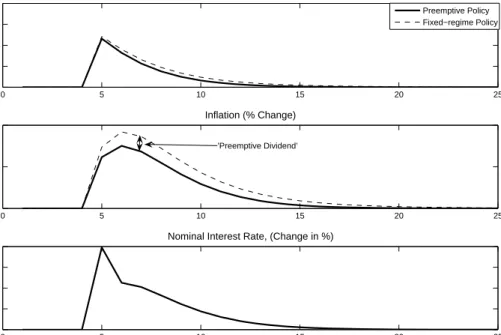
Using the baseline parameter values, figure 10 shows impulse responses to a demand

shock realized in period

t

= 5 under the endogenously switching preemptive policy

(solid line), and compares them to the fixed-regime policy (dashed line).

The

fixed-regime policy uses

α

= 1

.

5. The demand shock generates a delayed rise in inflation,

where the peak occurs the period following the shock under both policies. Under

both policies, the shock raises inflation and creates an expectation of higher future

inflation. This triggers a preemptive rise in rates that partially offsets the subsequent

rise in inflation and reduces output.

What does implementing a preemptive, threshold-switching policy buy the

mon-etary authority? We answer this question by isolating the expectations formation

effects that arise under the preemptive policy, but are absent from the fixed-regime.

Figure 11 mimics the shock intervention exercises in Leeper and Zha (2003) to create a

sequence of

i.i.d.

policy shocks

{

ε

ˆ

, that allows the fixed-regime policy,

i

=

α

π

+

ε

to exactly reproduce the interest rate path that the preemptive switching policy

im-plements (bottom panel). In the first two panels we see that under preemptive,

threshold-switching policy (solid lines), monetary policy is more effective than

fixed-regime policy (dashed lines): inflation rises by much less. The figure makes apparent

that in the case of a demand shock, output is stabilized also.

The magnitude of the total preemptive dividend for inflation—defined as the

differ-ence in the areas under the two inflation responses in figure 11 —varies with agents’

expectations of policy regime in periods after the initial disturbance. Expectations

of future regimes, in turn, vary with the size of the initial demand shock: the larger

the shock at

t

, the higher the probability that the preemptive state will be realized

at

t

+

k

, and the larger are the expectations formation effects. This is shown in

figure 12, which reports the long-run effect on the price level of a demand shock at

t

of a size given by the

x

-axis under preemptive policy (solid line) and fixed-regime

less-active policy (dashed line). As in figure 11,

i.i.d.

policy shocks are added to the

fixed-regime policy to match the interest rate path under switching. The long-run

13_{The nonlinear endogenous switching model has a stochastic steady state—defined as the state} the economy converges to when all shocks are set to zero—that differs from the linear model (where the steady state is zero inflation and zero output gap). For comparison, the impulse responses are reported with the non-zero steady state swept-out of the nonlinear model. Because the stochastic steady states for inflation and output are below zero, the figures understate the actual difference between policies.

preemption dividend for inflation increases monotonically with the size of the shock,

and can be quantitatively significant when demand shocks are large.

7.

Concluding Remarks

Endogenous switching of the monetary authority’s policy rule carries important

implications for how private agents form expectations. This paper has employed

threshold switching as a simple method for endogenizing policy regime changes that

has the appeal of resembling actual policy behavior in stylized form. Under

thresh-old switching, where policy rules change when endogenous variables cross specified

thresholds, symmetric shocks have asymmetric effects and the policy process

gen-erates quantitatively significant expectation formation effects. A preemptive policy

rule highlights the implications expectations formation effects have on equilibrium

outcomes. A monetary authority that stands ready to aggressively raise interest

rates in response to forecasts of rising inflation can shift expectations, enhancing

the effectiveness of efforts to stabilize inflation and output following demand shocks

when compared to a fixed-regime policy. We refer to the reduced volatility of inflation

following a demand shock as the “preemptive dividend.”

This line of work raises issues for further study. First, to what should the benefits of

preemptive policy be compared? This paper contrasts the effects under preemption

to those under a simple, time-invariant Taylor rule. In keeping with the

second-best policy perspective, it is interesting to contrast welfare under preemption with

threshold switching to “optimal implementable” policy rules, as in Schmitt-Grohe

and Uribe (2006).

Implementable rules are constrained to make policy instruments

respond to observable variables, rather than to exogenous disturbances.

A second issue emerges from the observation that in this paper, preemptive

thresh-old switching appears to offer a free lunch. It reduces the volatility of output and

inflation following demand shocks, but is not triggered by supply shocks for which the

preemptive policy would not uniformly reduce volatility. The difference arises because

supply shocks, in the calibration we used, do not generate hump-shaped responses

that would induce policy regime to change. Ultimately, the existence of humped

re-sponses is an empirical question. The present work suggests that the answer to the

question could have some practical implications for the behavior of monetary policy.

Endogenous regime change represents a new mechanism by which expectations

for-mation matters in determining the impacts of monetary policy. Given the magnitudes

of expectations formation effects that emerge from conventionally calibrated new

14_{In linear frameworks, the fully optimal monetary policy is linear in the exogenous shocks.} Clearly, endogenous switching policy cannot improve on optimal policies.

Keynesian models with threshold switching, conducting monetary policy to “manage

expectations” is potentially quite powerful.