Add-on Module
RF-FE-LTB
Lateral-Torsional Second-Order Analysis
of Members (FEM)
Program
Description
Version
August 2013
All rights, including those of translations, are reserved.
No portion of this book may be reproduced – mechanically, electronically, or by any other means, including photocopying – without written permission of DLUBAL SOFTWARE GMBH. © Dlubal Software GmbH Am Zellweg 2 D-93464 Tiefenbach Tel.: +49 9673 9203-0 Fax: +49 9673 9203-51 E-Mail: [email protected]
Contents
Contents Page Contents Page
1. Introduction 5
1.1 Add-on Module RF-FE-LTB 5
1.2 RF-FE-LTB Team 6
1.3 Using the Manual 7
1.4 Open the RF-FE-LTB Module 7
2. Theoretical Background 9
2.1 Preliminary Notes 9
2.1.1 General 9
2.1.2 Basis of the Calculation Method 11
2.1.3 Determination of the Initial Deformation 12
2.1.4 Calculation According to Second-Order
Analysis 12
2.2 Definitions 13
2.2.1 Coordinates and Displacements 13
2.2.2 Internal Forces 14
2.2.3 Single Springs and Continuous Springs 15
2.2.4 Loads 17
2.2.5 Boundary Conditions 19
2.3 Stress Calculation 19
2.4 Determination of Restrained Axis of
Rotation 22
2.5 Determination of Spring Stiffnesses 25
2.5.1 Rotational Springs 25
2.5.2 Translational Springs 27
2.5.3 Warp Springs 29
2.6 Analyses According to DIN 18800 32
2.6.1 Equivalent Member Method 33
2.6.1.1 Equivalent Member Analysis 34
2.6.1.2 Ultimate Limit State Analysis for Spatially
Imperfect Individual Member 36
2.6.2 Determination of Initial Deformations 37
2.6.3 Second-Order Ultimate Limit State
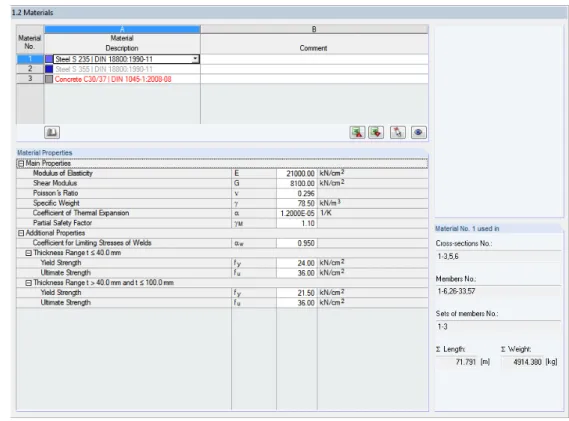
Analysis 38 2.6.4 Limit Loads FT or FG 39 3. Input Data 40 3.1 General Data 40 3.2 Materials 43 3.3 Cross-Sections 45 3.4 Nodal Supports 49
3.5 Elastic Member Foundations 55
3.6 Member End Springs 63
3.7 Member End Releases 67
3.8 Load 69 3.8.1 Nodal Loads 69 3.8.2 Member Loads 71 3.8.3 Imperfections 74 4. Calculation 77 4.1 Detail Settings 77 4.2 Start Calculation 79 5. Results 80 5.1 Stresses by Cross-Section 81
5.2 Stresses by Set of Members 83
5.3 Stresses by x-Location 83
5.4 Stresses by Stress Point 84
5.5 Internal Forces 85
5.6 Deformations 86
5.7 Support Reaction Forces 87
5.8 Critical Load Factors 88
6. Results Evaluation 90
6.1 Results on Cross-Section 91
6.2 Results on RFEM Model 93
6.3 Result Diagrams 97
6.4 Filter for Results 98
7. Printout 100
7.1 Printout Report 100
7.2 Graphic Printout 100
8. General Functions 102
8.1 Design Cases 102
8.2 Units and Decimal Places 104
8.3 Data Exchange 105
8.3.1 Material Export to RFEM 105
8.3.2 Export Cross-Section to RFEM 105
8.3.3 Export Results 105
9. Worked Examples 107
Contents
Contents Page Contents Page
9.1.1 Bending Without Rotational Restraint 107
9.1.2 Bending with Rotational Restraint 108
9.2 Beam Under Uniform Loading 109
9.3 Cantilevered Beam with Warping
Restraint 110
9.4 Cantilevered Beam Under Uniform Load 111
9.4.1 Crane Runway Beam with Free End 111
9.4.2 Cantilever End with Lateral Restraint 112
9.5 Beam Under Uniform Loading 112
9.6 Continuous Beam Under Two Nodal
Loads 113
9.7 Continuous Beam Under Uniform Loads 113
9.8 Three-Span Beam with Uniform
Loadings 115
9.9 Beam on Foundation with Axial Force 117
9.10 Roof Beam in Office Building 118
9.11 Beam with Eccentric Uniform Load 122
A Literature 123
1.
Introduction
1.1
Add-on Module RF-FE-LTB
The module RF-FE-LTB is not a stand-alone program but is integrated in the RFEM environ-ment as an add-on module. Thus, the model-specific input and loading data of all members is automatically available in the post-processing program. Conversely, the results from RF-FE-LTB can be graphically evaluated in the RFEM workspace and incorporated in the printout report. RF-FE-LTB carries out the check against lateral buckling and lateral-torsional buckling according to the finite elements method. The analysis is carried out on the entire structural system for no-tionally singled out sets of members. For this, the program determines the internal forces, de-formations, and stresses of spatially stressed structural systems according to the second-order analysis. Furthermore, RF-FE-LTB determines for a given load combination the stability load or the maximum resistance load while observing the normal, shear, and equivalent stresses. Separate design cases allow for a flexible analysis of lateral buckling and lateral-torsional buck-ling behavior.
According to DIN 18800, you can carry out the analysis according to various methods. RF-FE-LTB provides the following approaches:
• Calculation of the critical loads on a perfect system. This yields the
- Elastic flexural buckling load Ncr,z about the z-axis (out-of-plane),
- Elastic torsional buckling load Ncr,ϑ or
- Elastic critical moment for lateral-torsional buckling Mcr about the y-axis.
With these ideal values, you can carry out the stability analysis according to DIN 18800, Part 2 for I-sections according to the equivalent member method (e. g. with RF-LTB).
• Calculation of the ultimate capacity FT before a loss of stability occurs not exceeding the
predefined elastic limit stress (FT≤ FG) or determination of the elastic limit load FG, under
which the elastic limit stress is reached (FG≤ FT). The calculations are carried out on an
imperfect system.
• Stress analysis with the internal forces calculated under γ times the loads according to second-order analysis (imperfect system with loads Fd)
The calculation is carried out according to the lateral-torsional second-order analysis with the following possibilities:
• Analysis on entire system to take into account, for example, the restraining effects for structural components susceptible to LTB in a way that is appropriate for the system.
• Determination of imperfections by an eigenvalue analysis prior to the calculation and application of the scaled eigenvector as system initial deformation
• Consideration of the influence of bracings and other supporting structural components by placing eccentric nodal spring as well as idealization of warping restraints by means of according single springs
• Consideration of the elastic rotational restraint by trapezoidal sheeting (corrugated sheeting) of the roof membrane and/or bracing shear stiffnesses in the form of distrib-uted springs and rotational springs acting in both axes directions of the cross-section
• Realization of a possibly existing restrained axis of rotation by specifying appropriate boundary conditions
We hope you will enjoy working with RF-FE-LTB. Your DLUBAL Team
1.2
RF-FE-LTB Team
The following people were involved in the development of RF-FE-LTB:
Program coordination
Dipl.-Ing. Georg Dlubal Dipl.-Ing. (FH) Younes El Frem
Programming
Prof. Dr.-Ing. Peter Wriggers Dipl.-Ing. Georg Dlubal Mgr. Petr Oulehle
Dis. Jiří Šmerák Lukáš Tůma
Cross-section and material database
Ing. Ph.D. Jan Rybín Mgr. Petr Oulehle
Ing. Jiří Kubíček
Program design, dialog figures, icons
Dipl.-Ing. Georg Dlubal MgA. Robert Kolouch
Ing. Jan Miléř
Program supervision
Ing. Martin Vasek Ing. František Knobloch
M.Eng. Dipl.-Ing. (FH) Walter Rustler
Localization, manual
Ing. Fabio Borriello Ing. Dmitry Bystrov Eng.º Rafael Duarte Ing. Jana Duníková Dipl.-Ing. (FH) René Flori Ing. Lara Freyer
Alessandra Grosso Bc. Chelsea Jennings Jan Jeřábek
Ing. Ladislav Kábrt Ing. Aleksandra Kociołek
Ing. Roberto Lombino Eng.º Nilton Lopes Mgr. Ing. Hana Macková Ing. Téc. Ind. José Martínez MA Trans. Anton Mitleider Dipl.-Ü. Gundel Pietzcker Mgr. Petra Pokorná Ing. Michaela Prokopová Ing. Marcela Svitáková Dipl.-Ing. (FH) Robert Vogl Ing. Marcin Wardyn
Technical support, quality management
M.Eng. Cosme Asseya
Dipl.-Ing. (BA) Markus Baumgärtel Dipl.-Ing. Moritz Bertram
Dipl.-Ing. (FH) Steffen Clauß Dipl.-Ing. Frank Faulstich Dipl.-Ing. (FH) René Flori Dipl.-Ing. (FH) Stefan Frenzel Dipl.-Ing. (FH) Walter Fröhlich Dipl.-Ing. (FH) Wieland Götzler
Dipl.-Ing. (FH) Bastian Kuhn Dipl.-Ing. (FH) Ulrich Lex Dipl.-Ing. (BA) Sandy Matula Dipl.-Ing. (FH) Alexander Meierhofer M.Eng. Dipl.-Ing. (BA) Andreas Niemeier M.Eng. Dipl.-Ing. (FH) Walter Rustler M.Sc. Dipl.-Ing. (FH) Frank Sonntag Dipl.-Ing. (FH) Lukas Sühnel Dipl.-Ing. (FH) Robert Vogl
1.3
Using the Manual
Topics like installation, graphical user interface, results evaluation, and printout are described in detail in the manual of RFEM. The present manual focuses on special features of the add-on module RF-FE-LTB.
The description of the module follows the sequence and structure of the module's input and results window. The text of the manual shows the described buttons in square brackets, for example [View mode]. At the same time, they are shown on the left margin. In addition, ex-pressions that are used in dialog boxes, tables, and menus are set in italics to clarify the expla-nations.
The index at the end of the manual helps you find specific terms and subjects. However, if you still cannot find what you are looking for, please check our website www.dlubal.com where you can go through our FAQ pages by selecting particular criteria.
1.4
Open the RF-FE-LTB Module
RFEM provides you the following ways to open the RF-FE-LTB add-on module.
Menu
You can open the add-on module by using the RFEM menu:
Add-on Modules →Design - Steel→RF-FE-LTB.
Navigator
Alternatively, you can open the module in the Data navigator by double-clicking the entry
Add-on Modules → RF-FE-LTB.
Figure 1.2: Data navigator: Add-on Modules → RF-FE-LTB
Panel
If results from RF-FE-LTB are already available in the RFEM model, you can also open the add-on module in the panel:
Select the relevant RF-FE-LTB design case in the load case list located in the menu bar. Then, click [Results on/off] to graphically display the design criterion on the members.
On the panel, you can click [RF-FE-LTB] to return to the module.
2.
Theoretical Background
This chapter provides the theoretical background that is important for working with RF-FE-LTB. Basically, we introduce the theoretical approaches described in the literature. However, this in-troductory chapter cannot replace a textbook.
2.1
Preliminary Notes
2.1.1
General
Lateral-torsional buckling represents a stability case in which a primary flexural deformation is superimposed with a lateral displacement including torsion. Lateral-torsional buckling and flexural-torsional buckling are closely related terms. The difference is that lateral-torsion buck-ling is commonly associated with a stress from eccentric compression force, whereas flexural-torsional buckling is induced by bending. Furthermore, there is the case of compression bend-ing. In all cases, the position of the line of action of the loads applied to a member has a con-siderable influence on the magnitude of the stability load.
All mentioned stability problems can be analyzed in RF-FE-LTB. You can use different methods to calculate the lateral-torsional buckling of beams. Here are some of them:
• Equivalent member method according to DIN 18800, Part 1 and 2 (program RF-LTB [10])
• Calculation of eigenvalues (Mcr, Ncr) for continuous members or any frameworks subjected
to three-dimensional stress (program RF-FE-LTB)
• Limit load or stability calculation of frameworks subjected to three-dimensional stress ac-cording to second-order analysis on an imperfect system (program RF-FE-LTB)
• Limit load or stability calculation of frameworks subjected to three-dimensional stress ac-cording to a geometrically exact theory on the imperfect system
The equivalent member method is sufficiently accurate for many practical construction pur-poses. This method is described and verified in DIN 18800, Part 1 [7] and 2 [8] and many other publications. The method is implemented, for example, in the add-on module RF-LTB [10], where the lateral-torsional buckling analysis is carried out for members with monosymmetrical or doubly symmetrical I-section subject to uniaxial or biaxial bending and constant axial force. The equivalent member method according to DIN 18800 is limited in its application to particu-lar cross-sections (see above). In addition to this, you have to define boundary conditions for the equivalent member, which is not easy for general framework systems and therefore can only be estimated. For a more precise calculation, the framework subjected to three-dimen-sional stresses is to be computed by second-order analysis. Usually, this has to do with the calculation of the elastic stability load of a single-span or multi-span beam of a frame. The add-on module RF-FE-LTB is based on the finite element method and can be used to cal-culate the stability loads of members. Here, the elastic material behavior is assumed for a ge-ometric nonlinear behavior. The following basic assumptions apply for the warping torsional theory:
1. Shape-constant cross-sections to exclude local instabilities 2. Bernoulli bending
3. Moderate displacements or rotations that are small overall compared to the system dimensions
The calculations are three-dimensional according to the second-order analysis for flexural-torsional buckling, where the individual member elements are regarded as straight.
In the analysis, initial deformations can be taken as scaled eigenvectors of the system. Further-more, it is also possible to calculate eccentrically acting loads (for example load on top or bot-tom flange).
Depending on the geometric shape of the structural system, the actions, and the initial defor-mations (imperfections), different maximum failure and/or ultimate limit states can occur. Figure 2.1 presents the basic structural responses.
F FV FG f FT Fd Fki F/2 F/2 f
Figure 2.1: Structural responses
RF-FE-LTB gives the following results, as appropriate (see also Figure 2.1): 1. Critical load (bifurcation load) Fcr
• Elastic critical moment for lateral-torsional buckling Mcr,y • Elastic flexural buckling load Ncr,z
• Elastic torsional buckling load Ncr,ϑ
The program calculates always the smallest critical load of the system without consider-ing initial deformations. The elastic critical loads are required in the application of the equivalent member method (see chapter 2.6.1, page 33).
2. Ultimate capacity FT due to loss of stability (limit load) observing the elastic limit stress on
the imperfect system
The limit load FT is determined assuming a pure elastic material behavior with limitation
by an elastic limit stress to be defined. 3. Elastic limit load FG on imperfect system
This is a load that can be resisted by the system without that in any cross-section part the normal stress, the shear stress, or the equivalent stress (according to VON MISES) is greater than the respective limit stress. The calculation is to be carried out only in case of speci-fied initial deformations.
4. Possible limit load Fv due to loss of stability for specification of initial deformations
with-out observing the elastic limit stresses
5. Verification of the limit stresses under design loads Fd on the imperfect system according
to second-order analysis
Based on the second-order analysis, RF-FE-LTB can thus automatically find the critical, snap-through, or elastic limit loads. These loads are determined iteratively.
To determine the limit load FT or the elastic limit load FG (see Figure 2.1), an initial deformation
is to be applied to the system. In RF-FE-LTB, it is automatically generated from the first, lowest eigenmode (eigenvector), as this buckling mode corresponds to the lowest stability load. The scaling of this eigenmode is carried out according to DIN 18800 Part 2; however, it can also be user-defined (see chapter 2.6.2, page 37 and chapter 3.8.3, page 75).
RF-FE-LTB carries out analyses for all rolled sections, monosymmetrical and doubly symmet-rical I-sections, channels, T-sections, L-sections, rectangular sections, C-sections, hollow- and annular sections, as well as built-up cross-sections. Here, the stresses are determined accord-ing to the second-order analysis at the governaccord-ing cross-section points. The determination of the elastic limit load FG (see point 3 above) or the limit stress analysis (see point 5 above) is
based on these stress calculations.
Moreover, you can also analyze any cross-sections (for example SHAPE-THIN sections). They are directly imported from RFEM. Then, the stress analyses are run in the RF-FE-LTB module. Springs can be defined in RF-FE-LTB as single springs or continuous springs with an arbitrary point of application in the cross-section. As a rule, this is required when the stiffening effect of the roof cladding (for example trapezoidal sheeting) is to be taken into account.
Concentrated loads and line loads can act at arbitrary locations in the cross-section.
2.1.2
Basis of the Calculation Method
The theoretical basis of the program RF-FE-LTB is very extensive and cannot be discussed here in detail. The according background can be found, for example, in PETERSEN [2] or in RAMM, HOFMANN [11].
Usually, there are no analytical solutions for flexural-torsional problems that include nonlinear deformational dependencies. Therefore, the method of finite elements (FEM) is used in order to determine approximate solutions for the differential equations given in [2] or [11]. The pre-cision of the solution is dependent on the selected number of finite elements (see chapter 9.2). For the FE discretization, elements with two nodes are used. Cubic Hermite polynomials are applied within the elements for displacements in y- or z-direction and for the torsion about the x-axis. The longitudinal displacement in x-direction is described by an application of a linear polynomial. These applications solve the homogeneous differential equation of the corre-sponding linear analysis precisely, but are approximations for the second-order theory. The practical application of the method showed that usually eight elements per span of a beam are sufficient to calculate deformations with deviations of less than 5% from the convergent solu-tion. A solution is called convergent if there are no more changes in the solution in case of a doubled number of elements (see example 9.2, page 109).
Thus, we obtain a total of seven degrees of freedom per element node: ux, vy, wz, ϕx, ϕy, ϕz, ϕ‘x.
Where ux is the longitudinal displacement in the member direction; vy or wz is the displacement
in y- or z-direction, respectively; ϕx, ϕy, ϕz is the torsion about the x-, y-, or z-axis, respectively;
and ϕ‘x is the warping.
2.1.3
Determination of the Initial Deformation
The initial deformation is computed by solving the eigenvalue problem:(
K−λ⋅I)
⋅Φ=0 Equation 2.1: Eigenvalue analysisIn Equation 2.1, the stiffness matrix K is a function of the axial forces and moments of the basic load state. I is the unit matrix.
By solving the eigenvalue problems by an iterative method, we obtain the eigenvector Φ be-longing to the lowest eigenvalue; this eigenvector then determines the shape of the initial deformation. The scaling of the initial deformation is according to DIN 18800 Part 2.
2.1.4
Calculation According to Second-Order Analysis
For the second-order analysis, the following preconditions and assumptions are made:
• The cross-sections are thin-walled and constant within each portion.
• The individual member elements are regarded as straight.
• The shape of the cross-section shall remain unchanged in the deformation of the mem-ber. Thus, we exclude local instabilities, which possibly are also to be prevented by the stiffening of cross-sections.
• For bending, the BERNOULLI hypothesis applies stating that the cross-section remains
plane.
• The displacements and torsions are small compared to the dimensions of the system. The internal forces computed by second-order analysis are relative to the displaced and rotat-ed coordinate system and therefore do not nerotat-ed to be transformrotat-ed for the stress analysis. The analysis for a flexural-torsional problem can be carried out in different ways in RF-FE-LTB. The ways are the following:
1. Determination of the critical load factor on the undeformed system 2. Determination of the critical load factor on the deformed system 3. Analysis of the stresses under design load
4. Calculation of the maximum resisting load not exceeding the stresses
Basically, the calculation is iterative, with the stiffness matrix K changing due to the already computed internal forces and deformations. For the analyses according to the points 2, 3, and 4 described above, the eigenmodes are determined with the internal forces from the first step and considered according to chapter 2.6.2 before the actual iterative calculation.
The determination of the critical load factor according to point 1 or 2 gives the stability load of the analyzed structural system. In a numeric calculation, this load is characterized by the fact that either the determinant of the matrix K becomes zero, or that very high displacements oc-cur for very small load increases in the calculation. In both cases, the module RF-FE-LTB deter-mines that the corresponding state of equilibrium is no longer stable.
In the actual calculation, the program first computes the internal forces, deformations, and stresses for the load increments specified by the user (see chapter 2.3 Stress Calculation). At this point, there are two possibilities:
a) The load increments defined by the user are stable states of equilibrium. In this case, RF-FE-LTB automatically increases the load exceeding the defined maximum load until an instability occurs. The according value is then precisely determined by means of a nested iteration.
b) The load increments defined by the user cannot be reached all. In this case, RF-FE-LTB nests the load increment of the instability, starting from the last stable load increment. Thus, the critical load factor is known that belongs to the critical load Fcr (lateral-torsional
buckling load). For point 1 (see above), we thus obtain the lateral-torsional buckling load be-longing to the undeformed system. The maximum bending moment My thus corresponds to
the ideal lateral-torsional buckling moment. For point 2, we obtain the possible limit load FV
due to loss of stability. In both cases, the program does not check whether or not the limit stresses are observed. The stresses can be found in the results windows, where exceeded limits are highlighted.
The calculation of the system with initial deformation (see point 2 above) can also be carried out in a way that the limit stresses defined by the user are observed. In this case, RF-FE-LTB carries out the steps a) and b) and checks whether the limit stresses are observed.
Finally, it is also possible to carry out the second-order analysis on the system susceptible to lateral-torsional buckling under the design load (see point 3 above). If RF-FE-LTB can find an equilibrium in this case, then the design is directly verified if all limit stresses are observed. For examples of the presented cases, see chapter 9.
2.2
Definitions
2.2.1
Coordinates and Displacements
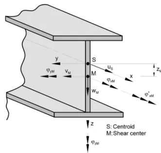
Figure 2.2 shows the cross-section coordinates and the positive displacement values.
The longitudinal displacement uS is related to the centroid S. In contrast, the displacements vM
and wM as well as the rotations ϕxM, ϕyM, ϕzM, and the warping ϕ‘xM are relative to the shear
cen-ter M. The displacements v, w, and u of an arbitrary cross-section point can be expressed with the linearization common in the second-order analysis by means of the displacement values of the shear center.
(
M)(
xM) (
M)
xM M(
M)
xM M y y 1 cos z z sin v z z sin vv= − − − ϕ − − ϕ ≈ − − ϕ
(
M)(
xM) (
M)
xM M(
M)
xM M z z 1 cos y y sin w y y sin ww= − − − ϕ + − ϕ ≈ + − ϕ
Equation 2.2: Displacement values
The displacement u of a point results from the translation of the cross-section in the x-direction, the rotation about the y- and z-axis and from the warping due to torsion:
o ' xM ' M ' M S w z v y u u= − − −ϕ ω
with ω0 Unit warping
Equation 2.3: Displacement values
2.2.2
Internal Forces
Figure 2.3 shows the used definitions of internal forces.
x y z S M Vy Mz Vz Mx Mω N My
Figure 2.3: Definitions on internal forces at the positive cut face
The shear forces Vz and Vy as well as the torsional moment Mx and the warping moment Mω are
relative to the shear center M; the bending moments My and Mz as the axial force N are relative
to the centroid S.
The internal forces are always related to the principal axes of the cross-section. For unsymmet-ric cross-sections, we therefore assume the shear forces Vv and Vu and the bending moments
2.2.3
Single Springs and Continuous Springs
Elastic supports can be modeled by considering centrically or eccentrically arranged single springs or/and continuous springs (element springs).
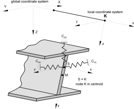
Figure 2.4 shows the centric single springs on node K. These springs are related to the global coordinate system (CSYS).
Figure 2.4: Centric nodal springs
The spring constants in Figure 2.4 mean:
CXK Nodal spring constant in global X-direction in [kN/cm]
CYK Nodal spring constant in global Y-direction in [kN/cm]
CZK Nodal spring constant in global Z-direction in [kN/cm]
CϕXK Nodal rotational spring constant about global X-axis in [kNcm]
CϕYK Nodal rotational spring constant about global Y-axis in [kNcm]
CϕZK Nodal rotational spring constant about global Z-axis in [kNcm]
The eccentric nodal springs at nodeK are relative to the local coordinate system: x y z S=K M CyK CzK zS yS CϕxK
Figure 2.5: Eccentric nodal springs
x,y,z Local coordinate system
CyK Nodal spring constant in local y-direction in [kN/cm]
CzK Nodal spring constant in local z-direction in [kN/cm]
CϕxK Rotational spring constant about local x-axis in [kNcm]
CωK Warp spring constant in [kNcm3] relative to the local x-axis (not shown in figure)
yS Distance of spring CzK from centroid S
zS Distance of spring CyK from centroid S
The continuous springs (element springs) are defined in Figure 2.6. These subgrade moduli are relative to the local coordinate system and constant along the member. In the program, they are related to the shear center M and recalculated.
y z M cy cz zS yS cϕx S x
Figure 2.6: Continuous springs
cy Nodal spring constant in local y-direction in [kN/cm]
cz Nodal spring constant in local z-direction in [kN/cm]
cϕx Rotational spring constant about local x-axis in [kNcm]
yS Distance of spring cz from centroid S
2.2.4
Loads
Figure 2.7 shows concentrated loads defined as centric nodal loads.
Figure 2.7: Centric concentrated loads
FX Concentrated load in global X-direction relative to M
FY Concentrated load in global Y-direction relative to M
FZ Concentrated load in global Z-direction relative to M
MX Concentrated moment about global X-axis, relative to M
MY Concentrated moment about global Y-axis, relative to M
MZ Concentrated moment about global Z-axis, relative to M
If the concentrated loads act centrically in the node K and point in the direction of the local coordinates, we have the simple option to specify these loads locally as eccentric loads (Figure 2.8) by setting the according coordinates to zero.
Eccentric concentrated loads at node K are to be related to the local coordinate system.
x y z S=K M yz Fz Fy zy
Figure 2.8: Eccentric concentrated loads
Fy Concentrated load in local y-direction
Fz Concentrated load in local z-direction
zy Distance of load Fy from centroid in z-direction
The following figure shows the definitions of the line loads.
Figure 2.9: Line loads
qx / qX Line load in local x- or global X-direction
qy / qY Line load in local y- or global Y-direction
qz / qZ Line load in local z- or global Z-direction
yS Local y-coordinate (relative to S) of the line load qz
zS Local z-coordinate (relative to S) of the line loads qy
mx / mX Local or global uniform torsional moment relative to S
The global line loads are automatically assumed to be acting in the shear center M, the local line loads are to be specified relative to the centroid S.
The line loads can be specified globally as well as locally. Eccentric line loads can only be de-fined as locally related. For the specification, the loads are relative to the centroid S. Within the program, they are converted to the shear center M.
The loads always relate to the main axes of the cross-section. For unsymmetric cross-sections, the concentrated loads Fu and Fv and the line loads qv and qu are to be assumed.
2.2.5
Boundary Conditions
The following figure shows the components of the displacement, torsion, and warping for specifying the boundary conditions.
Figure 2.10: Boundary conditions
The restraints of the structural system by the support reactions (boundary conditions) must be specified in the global direction, that is, they are related to the global axes X, Y, and Z. Thus, the individual translational and rotational components are set to zero or set free by specifying reference numbers.
2.3
Stress Calculation
RF-FE-LTB calculates the normal, shear, and VON MISES equivalent stresses at the governing
stress points iof the section. All rolled, built-up, and parametric thin-walled cross-sections of the library are permitted.
In the following equations, the stress points of the cross-section are indicated by the coordi-nates (yi, zi). All stresses are determined from internal forces that are calculated by
second-order analysis taking into account the partial safety factors for the actions.
The governing point for the determination of the stresses are dependent on the section-al shape. In Figure 6.4 on page 92, they are shown for an exemplary section. In the cross-section graphic, you can identify the stress point numbers listed in the output tables.
With the consideration of the warping torsion, for the normal stresses σx not only components
from axial force and bending, but also from the warping torsional moment occur. We obtain the following normal stress in a point i of the cross-section:
) z , y ( I M ) z , y ( S M ) z , y ( S M A N i i M i i z z i i y y i, x = + − − ω σ ω ω
Equation 2.4: Normal stress σx
The symbols mean:
Table 2.1: Parameter for normal stresses σx
The shear stresses are composed of shear force and torsional parts. The primary shear stresses
τp in a point i of the cross-section are determined as follows:
) z , y ( W M ) z , y ( s I ) z , y ( Q V ) z , y ( t I ) z , y ( Q V i i T p , x i i y i i y z i i z i i z y pi ⋅ + ⋅ + ⋅ ⋅ = τ
Equation 2.5: Primary shear stresses τp
The symbols mean:
Table 2.2: Parameters for primary shear stresses τp
Symbol Description
N Axial force
My Bending moment about y-axis
Mz Bending moment about z-axis
Mω Warping torsional moment
A Cross-sectional area
Sy(yi,zi) Section modulus about y-axis for point (yi,zi)
Sz(yi,zi) Section modulus about z-axis for point (yi,zi)
Iω Warping constant
ωM Main warping at point (yi,zi)
Symbol Description
Vy Shear force in direction of the y-axis
Vz Shear force in direction of the z-axis
Mx,p Primary torsional moment
Iy Second moment of area relative to y-axis
Iz Second moment of area relative to z-axis
Qy(yi,zi) Statical moment relative to y-axis for point (yi,zi)
Qz(yi,zi) Statical moment relative to z-axis for point (yi,zi)
t(yi,zi) Thickness of the governing cross-section parts in point (yi,zi)
s(yi,zi) Thickness of the governing cross-section parts in point (yi,zi)
Furthermore, it is possible to calculate the secondary shear stress τs due to the secondary tor-sional moment Mx,s.
(
)
(
i i)
i i s , x i s z , y t I z , y A M ⋅ ⋅ = τ ω ωEquation 2.6: Secondary shear stress τs
The symbols mean:
Table 2.3: Parameter for secondary shear stresses τs
The calculation of the secondary shear stresses is possible for rolled cross-sections, mono-symmetrical and doubly mono-symmetrical I-sections, and box sections.
In RF-FE-LTB, it is up to you to decide whether or not the secondary shear stresses are to be taken into account in the stress calculation. If they are to be included in the stress calculation, they are directly added to the primary shear stresses.
The Equivalent stress σeqv according to VON MISES is determined from the normal and shear
stress as follows: 2 i s , p 2 x eqvi= σ +3τ σ
Equation 2.7: Equivalent stress σeqv
In the standard case, it is assumed for the calculation of the equivalent stresses that the sec-ondary shear stresses may be neglected. However, if they are considered (see above), the sum from primary and secondary shear stress is taken for τp,s. The shear stresses due to primary
tor-sional moment according to Equation 2.5 are always considered in Equation 2.7.
The normal, shear, and equivalent stresses are calculated for all points in the cross-section that can be governing for the three-dimensional stress resulting in lateral-torsional buckling. In the output, the location where the maximum value occurs for every type of stress (normal, shear, and equivalent stress) is shown.
In the limit load calculation, the limit load FG is calculated for which at no location in the
cross-section the allowable values for the stresses due to γ times the actions are exceeded. To this end, it is necessary to determine the maximum stress in the cross-section. Thus, the following conditions are to be satisfied:
M k , y i eqv i M k , y i s , p i M k , y i x i f ) ( max ; 3 f ) ( max ; f ) ( max γ ≤ σ ∗ γ ≤ τ γ ≤ σ
Equation 2.8: Conditions for the limit load FG
If the design is carried out according to DIN 18800 Part 2, element (121) and Part 1, element (749), then the normal or equivalent stresses may exceed these limit values by 10 % (see chapter 2.6.1).
Symbol Description
Mx,s Secondary torsional moment
Aω(yi,zi) Warping area in point (yi,zi)
Iω Warping constant
2.4
Determination of Restrained Axis of Rotation
In practical constructions, there is often a constructively caused lateral-torsional problem with restrained axis of rotation (translational restraint) at a distance zD of the centroid. This restrainedrotational axis is implemented as continuous or discrete translational springs in y-direction. For the spring stiffnesses, values of the magnitude 108 through 1010 for c
y are to be taken to
sup-press the displacements in the restrained axis of rotation.
Figure 2.11: Torsional restraint
The translational restraint may be taken according to DIN 18800 Part 2 [8] in the design of a sufficient lateral restraint of deformation. To achieve a sufficient restraint, you can, for exam-ple, use masonry permanently connecting to the compression flange. If trapezoidal sheets according to DIN 18807 [13] are connected to the girder and the condition
S req S
prov ≥
Equation 2.9: Condition for shear panel stiffness
where 2 p 2 p 2 2 z T 2 2 a h 70 h L 4 I E I G L I E S S req π + + π = = ω
Equation 2.10: Required shear panel stiffness for attachment in every groove
for an attachment in every groove (rib) is satisfied, then the point of connection must be seen as rigidly fixed in the plane of the trapezoidal sheeting.
Sa refers to the portion of the shear strength of the trapezoidal sheeting for the analyzed beam
according to DIN 18800 Part 1 [7] in case of attachment in every rib. Here, L is the span width of the beam to be braced and hp is the depth of the beam (provided that it is an I-section).
If the trapezoidal sheeting is fastened only in each second rib, then the following applies: a b 5 S S S req = = ⋅
Where Sa see Equation 2.10
Equation 2.11: Required shear panel strength for fixation in every second groove
Equation 2.10 and Equation 2.11 for the determination of the lateral restraint of a beam (trans-lational restraint) can, in case of an according type of the points of connection, used for other sheeting than trapezoidal sheeting, see note on DIN 18800 Part 2, element (308).
The ideal shear modulus of a trapezoidal sheet is given as:
+ = m kN L K 100 K 10 G s 2 1 4 s
where K1 Shear panel value according to approval in [m/kN]
K2 Shear panel value according to approval in [m2/kN]
LS Shear panel length in [cm], see Figure 2.12
Equation 2.12: Shear modulus of trapezoidal sheeting
Thus, it follows for the shear stiffness part of the beam to be braced (for example frame beam in Figure 2.12):
[ ]
kN G 100 a ST= swhere a Distance of the beam to be braced (frame beam) in [cm]
Equation 2.13: Shear stiffness of trapezoidal sheeting
The shear strength of the wind bracings and stabilizing bracings can also be considered. For the ideal shear stiffness of one bracing with connections without slip, we obtain (see [8] and [1]): α ⋅ ⋅ + α ⋅ α ⋅ ⋅ = cot A E 1 cos sin A E 1 1 S P 2 D V
where SV Shear stiffness of bracing in [kN]
AD Area of the diagonal in [cm]
AP Area of posts in [cm]
α Angle between diagonal and frame beam flange
Equation 2.14: Shear stiffness of bracing
In the equation above, only the tension diagonals of the cross bracing are considered. If differ-ent posts or diagonals are intended, the minimum cross-section areas are to be taken for AP or
AD.
Equation 2.14 can be converted as follows.
P 3 D 3 2 2 2 V A a A b a E b a S + + =
Equation 2.15: Shear stiffness of bracing
Thus, it is possible to approximately calculate the shear stiffness for one frame beam or girder (only from bracings).
V s R S L a m S =
where m Number of stiffening bracings in roof plane
Equation 2.16: Shear modulus of trapezoidal sheeting
If the shear stiffnesses from trapezoidal sheeting and bracing are applied at the same time, we obtain from Equation 2.10, Equation 2.14, Equation 2.15, and Equation 2.13:
• Connection in every groove: R
T S S S prov = +
Equation 2.17: Shear panel stiffness
• Connection in every second groove R T S S 5 1 S prov = +
Equation 2.18: Shear panel stiffness
The analysis is then run according to Equation 2.9.
In RF-FE-LTB, a continuous translational restraint is to be accordingly idealized by continuous lateral translational springs cy with a high stiffness, for example 106 (kN/cm)/cm. An example
Laterally adjacent members that are fixed in the longitudinal direction (for example single purlins resting on the frame beam) can be idealized by discrete single springs cy in those
points, for example as follows: L
A E cy= ⋅
where L Length of purlin up to the support point E Modulus of elasticity
A Cross-sectional area of purlins
Equation 2.19: Translational spring by single support
If the check of a translational restraint according to DIN 18800 Part 2 is not fulfilled, it is possible to determine a continuous translational spring by means of the determined ideal shear stiffness
prov S (see chapter 2.5.2).
2.5
Determination of Spring Stiffnesses
2.5.1
Rotational Springs
The calculation of the provided rotational restraint coefficient is based on the model of several springs placed one behind the other (see [8], [14]).
k , P k , A k , M k , c 1 c 1 c 1 c rov p 1 ϑ ϑ ϑ ϑ + + =
Equation 2.20: Effective rotational restraint
For simplification, Equation 2.20 in DIN 18800 is expressed with the characteristic values. The symbols of this equation are described in the following.
Rotational restraint c
ϑM,kfrom supporting structural component
k a
I E cϑM,k= ⋅a⋅
Equation 2.21: Rotational restraint from supporting structural component
The value cϑM,k represents the theoretical rotational restraint from bending stiffness Ia of the
supporting structural component a assuming a rigid connection. Furthermore, the following is valid for Equation 2.21:
Ia Moment of inertia of the supporting structural component in [cm4/cm]
A Span of the supporting structural component in [cm]
K Coefficient: k = 2 for single-span and double-span beams, end-span beams k = 4 for continuous beam with three or more spans
For a noncontinuous rotational restraint (for example by purlins), the moment of inertia Ia of the
supporting structural component is converted to a continuous support according to Ia = I / e,
where e is the distance of the supporting single-span beams (for example purlins).
If the supported beam can rotate only in one direction, the cϑM,k value may be multiplied by
factor 3.0 according to Equation 2.21. This is the case if, for example, a supported beam is part of the structure of an inclined roof.
Rotational restraint c
ϑA,kfrom deformation of the connection
cϑA,krepresents the rotational restraint from deformation of the connection. For connections of
single girders by means of bolts without slip (alternatively left and right from web of the cross-section to be stiffened), we can assume a rigid connection as approximation, that is, cϑA,k is
equal to infinity and is discarded in Equation 2.20.
For rotationally elastic support by means of trapezoidal sheeting, we obtain:
0 . 2 10 b 1.25 for 10 b c 25 . 1 c 25 . 1 10 b for 10 b c c 1 1 k , A k , A 1 2 1 k , A k , A ≤ < = ≤ = ϑ ϑ ϑ ϑ
Width b1 Width of the top flange of the supported beam in [cm]
Equation 2.22: Rotational restraint from deformation of the connection
The characteristic value for the joint stiffness cϑA,k of steel trapezoidal sheeting profiles is taken
from Table 7 of DIN 18 800 Part 2. This table is included in the program.
If ratio b1/10 > 2.0, the ratio in the equation above is limited to 2.0 in order to be on the safe
side. According to OSTERRIEDER [8] (note in paragraph 4), is also possible to specify values for
k , A
cϑ that are greater than those given by Table 7 . This option is also available in the program.
If the coefficient cϑA,k is determined according to Table 7 and the trapezoidal sheeting profiles
show thicknesses t greater than 0.75 mm, we obtain greater joint stiffnesses. Approximately, the table value may be increased by a factor as follows [15]:
2 prov 75 , 0 t tprov in [mm]
Equation 2.23: Increase factor for thicknesses > 0.75
Rotational restraint c
ϑP,kfrom cross-section deformation
cϑP,k is the torsional restraint due to deformation of the supported beam section. It is obtained
as follows [15]. 3 1 1 3 m 2 k , P t b 5 . 0 s h 1 ) 1 ( 4 E c ⋅ + ⋅ µ − ⋅ = ϑ
Where b1, t1 Width or thickness of the top flange of the supported beam in [cm]
S Web thickness of the supported beam in [cm] hm Distance of the flange's centerline in [cm] µ Poisson's ratio of steel with the fixed value µ = 0.3
Equation 2.24: Rotational restraint from distortional buckling
The determination of cϑP,k according to Equation 2.24 in [15] necessarily requires that in the
case of a noncontinuous rotational restraint, the concentrated loads from the supported struc-tural component (transferred to the supported beam) reach only a maximum of 50 % of the limit loads for constructions without stiffeners (see for example [7]). Further values can be found in the manual RF-LTB [10] and in the commentary [15], page 169.
The continuous rotational springs according to Equation 2.20 (cϑ,k = cϑ,x) can be used as
dis-crete rotational spring (single spring) if the continuous spring is multiplied by the correspond-ing influence width.
2.5.2
Translational Springs
For the frequent case of a beam span (for example frame beam, platform beam, or floor beam) stabilized by one or several bracings, the translational springs can be determined cy according
to PETERSEN [2] as follows: π ⋅ = m m / kN L S prov cy 22
where prov S Part of the shear stiffness of a beam according to Equation 2.17 or Equation 2.18
L Length of bracing
Equation 2.25: Translational spring constant
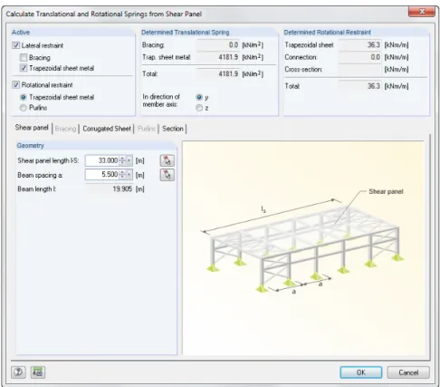
Figure 2.13: Frame beam with trapezoidal sheeting and bracings
The bracing should have a regular structure, because the equation for cy is derived by a
"uni-form smearing" of the bracing over the length L.
The shear stiffnesses from bracing and trapezoidal sheeting may be added only if the beams that are to be restrained by laterally connected sections resistant to compression and the trapezoidal sheets above are connected to the bracing:
Figure 2.14: Stiffening by trapezoidal sheeting and compression sections
Thus, the trapezoidal sheeting and the bracing act as parallely placed springs that can be add-ed up to a global spring. If the beams are connectadd-ed only by supporting purlins with each oth-er (which, convoth-ersely, are possibly supported by trapezoidal sheeting), then only the part SR
(see Equation 2.16) from the bracing is taken for prov S.
An example for the determination of a lateral translational spring cx is given in PETERSEN [2]
chapter 7.17.3. In [2] and in the Stahlbau Handbuch [17], chapter 3.2, you can find further information for the determination of equivalent stiffnesses.
Compression connection to bracing Trapezoidal
2.5.3
Warp Springs
The restraint of the warping increases the torsional stiffness of a girder with a thin-walled open cross-section. This increase can be considered by discrete warp springs Cω.
Warping restrained by an end plate [4], [10]
In this case, the warp spring is given according to Equation 2.29 as follows: 3 t h b G 3 1 Cω= ⋅ ⋅ ⋅ ⋅
Equation 2.26: Warp spring by end plate
Figure 2.15: Warp spring from end plate
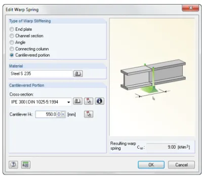
Warping restraint by a cantilevered portion [2]
The warp spring due to a cantilevered portion is determined acc. to the following equation: ) L ( tanh 1 I G Cω= ⋅T⋅λ⋅ λ⋅ k where ω ⋅ ⋅ = λ I E I G T
Lk Length of cantilevered portion
Equation 2.27: Warp spring from cantilevered portion
lk
w = 0 x
y z
Warping restraint by means of a diaphragm resistant to torsion
The warp springs from the end plates or cantilevered portions results only in a relatively small restraint. The intended installation of cross-stiffenings resistant to torsion in the form of weld-ed channel sections or angles is more effective[2]. This results in a closweld-ed box section about the z-axis (vertical axis)
b u t s hm hu
Figure 2.17: Warp spring from cross-stiffening
(
)
+ ⋅ ⋅ ⋅ = ⋅ ⋅ ⋅ =∑
ω s h t b 2 t b 4 h G t L A 4 h G C u u 2 u u i i 2 mwhere Am Area enclosed by the centerline
∑
i i t L
Sum of the side lengths divided by the respective plate thickness
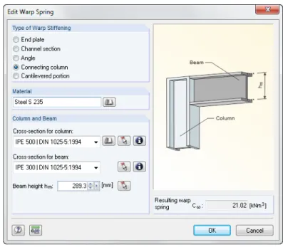
Warping restraint by a column connection
The warp spring Cω for the frame beam can be calculated according to the basic expression:
3 m t h b G 3 1 Cω= ⋅ ⋅ ⋅ ⋅
where G Shear modulus
IT Torsional moment of inertia for • closed sections:
∑
= i i 2 m Bredt , T t L A 4 IAm area of the section enclosed by the centerline • open sections: + ⋅ =
∑
5 i i i i 3 i i . Ven . St , T 31L t 1-0.63Lt 0.052 Lt IThe expression in the brackets is a correction factor that takes into account the solidness of individual rectangular components (length Li,
thickness ti). For thin-walled sections, this factor can be taken as 1.0.
hm Distance of the flange centerlines
Equation 2.29: Warp spring from column joint
hm
2.6
Analyses According to DIN 18800
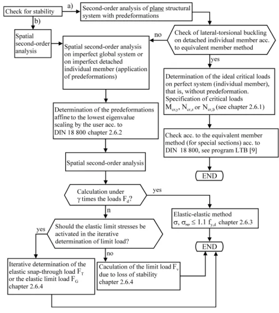
The following chart shows the possible analyses that are supported by RF-FE-LTB and compli-ant with DIN 18800.
Figure 2.19: Analyses according to DIN 18800 with RF-FE-LTB a) Plane second-order analysis
b) Spatial second-order Analysis
The calculation of the critical load factor on the global system according to the second-order analysis or the check of the elastic limit stresses under (γ times) design loads according to sec-ond-order analysis of the global structural system should always be preferred to the equivalent member method, as the real boundary or transition conditions are considered on the global structural system.
The ideal critical loads whose values are included in the equivalent member method can also be determined in RF-FE-LTB for the global system (that is, more precise than by means of ana-lytical expressions that consider the boundary and transition conditions only approximately), but the critical loads can be qualified precisely (see example in chapter 2.6.1).
2.6.1
Equivalent Member Method
For simplification according to DIN 18800 Part 2, the analyses for lateral buckling and lateral-torsional buckling are carried out separately. As a rule, the analysis of the lateral buckling (see the following figure) is carried out in the plane of the structural system by calculating the plane structure according to second-order analysis as stress analysis under the design loads and by applying the initial deformations.
Figure 2.20: Analysis of a structure: flexural buckling in the plane and lateral-torsional buckling for an individual member
The analysis of the lateral-torsional buckling is performed on a notionally singled out indi-vidual member with the following boundary conditions and loads:
• Loads
The individual member is loaded by the design loads and at the member ends by the in-ternal forces determined on the global structural system.
• Geometrical boundary conditions and elastic supports
The kinematic conditions that you can see when cutting out the individual member from the global system are to be specified as boundary conditions, especially those regarding the deflection perpendicular to the plane of the structural system and the torsional re-straints. Elastic supports by adjacent structural components can be considered by means of equivalent springs according to chapter 2.5.
For an individual member defined in such a way, there are two possibilities for the lateral-torsional analysis (see also Figure 2.19):
2.6.1.1 Equivalent Member Analysis
The simplified analysis according to DIN18800 Part 2, elements (306), (307), (311), (320), and (323) is essentially limited to doubly symmetrical or monosymmetrical I-sections (see element (311), note 1). In addition to this, this verification format can be used only for specific loads that are based on the following ideal critical values:
Mcr,y Elastic critical moment for lateral-torsional buckling according to elasticity theory for
the sole action of moments My without axial force
Ncr,z Axial force under the smallest critical buckling load according to elastic theory (the
smallest load from buckling about the z-axis or lateral-torsional buckling about this axis, or torsional buckling, see for example manual for program RF-LTB [9].
In RF-FE-LTB, you can calculate these ideal critical loads also on the undeformed individual member (perfect system). The program always gives the smallest critical buckling load. In the equivalent member method, however, the values Mcr,y and Ncr,z are used. Hence, it is necessary
to check whether the critical buckling load calculated by the program corresponds to these values (see also example 9.9 on page 117, where Ncr,y is smaller than Ncr,ϑ).
Example
x 6 m Nd = 700 kN U 400, St 52 y z S Left support: u = v = w = φx = 0 Right support: v = w = φx = 0Centric compression force: Nd = 700 kN
Figure 2.21: Channel section with centric compression force
For lateral buckling, the following critical loads result: kN 3 . 590 , 6 800 350 , 20 000 , 21 L I E N z2 2 2 2 z , cr = π ⋅ = π ⋅ ⋅ = kN 0 . 274 800 846 000 , 21 L I E N 2 2 2 2 y y , cr = π ⋅ = π ⋅ ⋅ =
Equation 2.30: Critical loads
The elastic torsional buckling load Ncr,ϑ according to [10] is determined according to the
following equation. 2 z 2 eqv 2 z , cr i I E N ⋅ λ π ⋅ ⋅ = ϑ
To solve Equation 2.31, the equivalent slenderness λeqv is necessary.
(
)
(
)
8939.5 04 . 16 54 . 10 21 . 15 54 . 10 4 1 54 . 10 2 04 . 16 54 . 10 9 . 14 800 i c i c 4 1 c 2 i c i L 2 2 2 2 2 2 2 2 2 2 2 M 2 2 p 2 2 2 M 2 2 z 2 eqv = + ⋅ ⋅ + ⋅ ⋅ + ⋅ = + ⋅ ⋅ + ⋅ ⋅ + ⋅ = λ 5 . 94 eqv= λ ⇒Equation 2.32: Equivalent slenderness
The slenderness values in Equation 2.32 are determined as follows: cm 21 . 15 04 . 3 9 . 14 i i ip= 2y+2z = 2+ 2= cm 11 . 5 zM=− cm 04 . 16 ) 11 . 5 ( 21 . 15 z i iM= 2y+ 2M= 2+ − 2 =
Equation 2.33: Slenderness values
c is the so-called twisting radius.
2 2 2 z T 2 2 z 2 111.15cm 20350 000 , 21 6 . 81 100 , 8 800 350 , 20 000 , 221 I E I G L I I c = ⋅ ⋅ ⋅ π + = ⋅ ⋅ ⋅ π + = ω cm 54 . 10 c= ⇒
Equation 2.34: Twisting radius
Thus, it is possible to compute the elastic torsional buckling load according to Equation 2.31. kN 2 . 125 , 2 9 . 14 5 . 94 350 , 20 000 , 21 Ncr, 2 2 2 = ⋅ π ⋅ ⋅ = ϑ
Equation 2.35: Elastic torsional buckling load
Ncr,y is the lateral buckling load about the y-axis in the plane of the structural system, Ncr,z is the
lateral buckling load for buckling about the z-axis (that is, deflection in the direction of the y-axis). Ncr,ϑ represents the torsional buckling load: the cross-section in y-direction is displaced
and at the same time rotated about the longitudinal x-axis. Since Ncr,ϑ is smaller than Ncr,z, this
value is governing for the check of the equivalent member according to element (306) and (304). Buckling curve c → α = 0.49 017 . 1 9 . 92 5 . 94 a k k=λλ = = λ
[
1 0.49(1.017 0.2) 1.017]
1.217 5 . 0 k= ⋅ + ⋅ − + 2 = 530 . 0 017 . 1 217 . 1 217 . 1 1 2 2 z = − + = κkN 5 . 2994 5 . 91 1 . 1 36 Npl,d= ⋅ =
Equation 2.37: Plastic axial force
Check: 0 . 1 44 . 0 5 . 2994 53 . 0 700 N N d , pl z d = ≤ ⋅ = ⋅ κ
Equation 2.38: Plastic axial force
Thus, the check against lateral-torsional buckling would be fulfilled, while the check for lateral buckling about the y-axis would fail because Nd = 700 kN > Ncr,y = 274 kN.
The program RF-FE-LTB gives the smallest critical load factor Ncr,y = 274 kN. To determine the
governing critical load for deflection in y-direction, you might have to apply a mid-span sup-port in z-direction (wx=l/2 = 0). The resulting values are shown in the following table:
Table 2.4: Critical buckling loads
The ideal values Mcr,y (without axial force!) and Ncr,z or Ncr,ϑ (under the sole action of a centric
axial force) must be determined separately with RF-FE-LTB, that is, in two calculation runs at the respective perfect system.
This example shows the problem of the equivalent member method. A better method is the second possibility for the individual member presented in the following chapter.
2.6.1.2 Ultimate Limit State Analysis for Spatially Imperfect Individual Member
As an alternative design method, you can use the calculation of the spatially imperfect indi-vidual member according to second-order analysis of elasticity according to element (121) together with element (201) in RF-FE-LTB.
In case of a stable equilibrium, the maximum equivalent stress must be smaller than the limit stress fy,d. In small portions, the equivalent stress may exceed the limit stress fy,d by 10% (see
chapter 2.6.3, page 38). The imperfections are to be applied in compliance with DIN 18800 Part 2 (see the following chapter 2.6.2). Thus, the procedure corresponds to the elastic-elastic method.
Ncr analytical
RF-FE-LTB wl/2
≠
0 273.8 kN Ncr,y = 274.0 kN2.6.2
Determination of Initial Deformations
According to DIN 18800 Part 2 for the second-order analysis for considering geometrical and structural imperfections, geometrical equivalent imperfections are to be specified. For un-braced systems, these are usually initial sway imperfections caused by angles of bar rotation. For braced systems, these are initial bow imperfections (initial camber)in the form of sinus-oidal or parabolic half-waves.
The shape of the initial deformation should be taken affine to the lowest buckling or lateral-torsional buckling eigenmode, see element (202). According to the commentary to DIN 18800 [15], it is sufficient to select the initial deformation in such a way that a sufficiently great com-ponent of the lowest eigenmode is included. Thus, the program aims at ensuring that the load-deformation-curve tends towards the first eigenvalue.
To this end, RF-FE-LTB calculates the eigenmode belonging to the smallest eigenvalue (prelim-inary eigenvalue analysis) and chooses it as deformation mode (imperfection shape). The de-formation modes in the direction of the main axes y and z are analyzed and the deflection di-rection belonging to the smallest eigenvalue is chosen (initial deformation in y-didi-rection vv, in z-direction wv). Taking into account these initial deformations, bending moments result on the uniformly loaded beam about both cross-section axes as well as torsional moments.
Next, the imperfection is considered by a user-defined scaling of the eigenmode. For this pur-pose, the following menu options are available in the program (see chapter 3.8.3, page 75):
• Direct numerical specification of the maximum camber rise of the initial deformation by a graphical representation of the eigenvector and the location of the maximum displace-ment.
• Calculation of the camber rise (initial bow imperfection) according to element (204), Table 3 with the user-defined governing buckling curve and the reference length; furthermore, the calculation of the initial sway imperfection according to element (205) considering the reduction factors r1 and r2. In determining the initial sway imperfection, the user specifies
the required data (like reference length and number n of the mutually independent caus-es for the initial sway imperfections of members).
The initial deformations to be taken according to [3] chapter 2.2 and 2.3 may be reduced under certain conditions. In RF-FE-LTB, you have the following options:
Reduction 1) according to element (201)
For the elastic-elastic method, camber rises of the bow imperfections or the initial sway imper-fections ϕ0, which depend on the buckling curve, may be reduced by the factor 2/3.
Reduction 2) according to element (202)
In the lateral-torsional buckling analysis, the amplitudes of the initial bow imperfections out of the principal stress plane may be reduced by another 50 %.
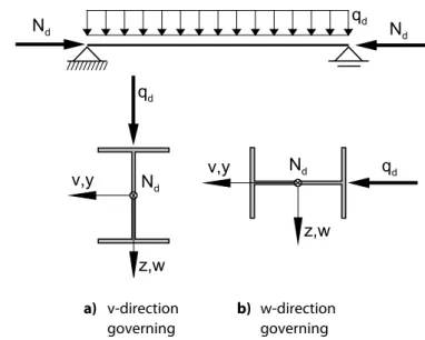
The reduction option 2) is not without its problems, as this reduction may be carried out only if the initial deformation mode for the lateral-torsional buckling belongs to the smallest eigen-mode. This effect is illustrated in the following Figure 2.22.
v,y z,w Nd Nd qd qd Nd Nd qd v,y z,w a) v-direction b) w-direction governing governing
Figure 2.22: Governing initial deformation for the reduction according to DIN 18800 Part 2, element (202).
RF-FE-LTB analyzes both principal axes directions y and z. This is because depending on the spatial arrangement of the member and the load constellation, either the w- or the v-direction can be governing for the lateral-torsional buckling.
In case a), v corresponds to the direction of deflection for the lateral-torsional buckling. If the lowest eigenmode belongs to this direction, a reduction by 50 % is allowed.
In case b), the displacement mode w can be imagined as the initial deformation mode in the direction of v according to DIN 18800 Part 2. Thus, a reduction by 50 % may be carried out only if the eigenmode of the lowest eigenvalue (which is to be scaled by the user) runs in the w-direction.
To learn more about the determination of the initial deformation, see chapter 3.8.3.
2.6.3
Second-Order Ultimate Limit State Analysis
RF-FE-LTB determines the internal forces according to the second-order analysis taking into account spatial initial deformations (see chapter 2.6.2).
For the elastic-elastic method: according to DIN 18800 Part 2, element (121), it is necessary to verify that under the design actions (γF times the loads) the following conditions are met
M k , y d , y v d , y d , y x f f max f 3 1 max ; f max γ = ≤ σ ≤ τ ≤ σ
Equation 2.39: Design conditions for stresses
According to DIN 18800 Part 1, element (749), the equivalent stress may exceed the limit stress
σeqv by 10 % in isolated points.
d , y eqv 1.1f maxσ ≤
For members subjected to axial force and bending, an "isolated point" can be assumed if the following is valid at the same time:
d , y z z d , y y y f 8 . 0 y I M A N and f 8 . 0 z I M A N ≤ + ≤ +
Equation 2.41: Allowance for locally limited plastification
As a rule, the maximum stress occurs on a cross-section edge at which the shear stresses from the shear forces become zero. Thus, the analyses are reduced to the analysis of the normal stresses.
2.6.4
Limit Loads F
Tor F
GRF-FE-LTB also offers the option to carry out the ultimate limit state analysis by comparing the limit loads (ultimate capacity) with the design loads Fd. Only the following analysis is of
practi-cal importance: d G d T F orF F F ≥ ≥
Equation 2.42: Design conditions for ultimate loads
The program determines the load level FT or FG by an iterative load increase (see Figure 2.1,
page 10).
FT Ultimate capacity due to loss of stability (limit load) on the imperfect system not
ex-ceeding the elastic limit stress
FG Elastic Limit Load on imperfect system (all shear, normal, and equivalent stresses are
less or equal to the respective elastic limit stress)
RF-FE-LTB additionally allows you to calculate the limit load FV due to initial deformations
without observing the elastic limit stress. This ultimate load, however, is only of theoretical interest.
3.
Input Data
After you start the add-on module, a new window appears. The navigator on the left shows the available module windows. Above the navigator, you find a drop-down list with the design cases (see chapter 8.1, page 102).
You must define the design-relevant data in several input windows. When you open RF-FE-LTB for the first time, the following RFEM data is imported:
• Sets of members
• Load cases and load combinations
• Materials
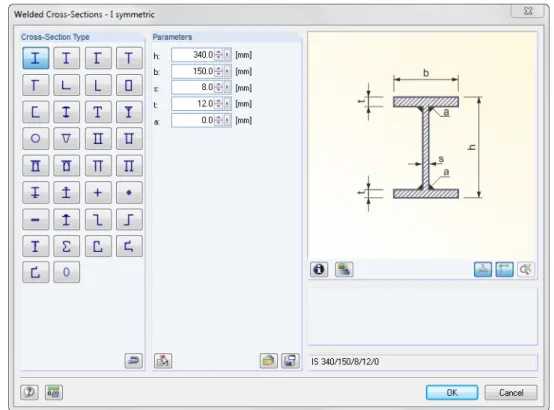
• Cross-sections
The sets of members are considered as notionally singled out from the model, that is, they are not coupled to the members in the RFEM model. Changes of cross-sections and the geometry are automatically compared with RF-FE-LTB. Imperfections from RFEM are not imported. To go to a particular module window, click the according entry in the navigator. To go to the previous or next module window, use the buttons shown on the left. Alternatively, you can al-so press the function keys [F2] (forward) and [F3] (backward) to browse through the module windows.
To save the input, click [OK]. Thus, you exit RF-FE-LTB and return to the main program. To exit the module without saving the data, click [Cancel].
3.1
General Data
In the 1.1General Data window, you specify the sets of members and actions for the design.
Figure 3.1: Window 1.1 General Data
Design of
Figure 3.2: Analysis of sets of members
Only sets of members of the 'continuous members' type can be analyzed. If sets of members are already defined in RFEM, it is possible to enter their numbers in the list or to select them graph-ically in the RFEM work window upon clicking []. By selecting the All check box, you can select all sets of members available in the model for the design.
The design is only possible for the set of members type 'continuous members' (with connected members that do not branch out). A set of members of the type 'group of members' leads to an error message before the calculation.
Figure 3.3: Error message when designing a group of members
To define a new set of members, click [New]. The dialog box known from RFEM appears where you specify the parameters of the set of members.
During the design of the set of members, the members are analyzed as cut out from the system. Here, you must consider the boundary conditions of a built-up column or a complete frame as a whole. This is done in the other input windows of RF-FE-LTB.
Existing Load Cases and Combinations
This section lists all load cases and load combinations created in RFEM.
To transfer the selected entries to the To Design list on the right, click []. Alternatively, you can double-click the relevant entry. To transfer the entire list to the right, click [].
To make a multiple selection, select the load cases while pressing [Ctrl], as common in Windows. Thus, you can transfer several load cases at once.
If a load case is marked by an asterisk (*), for example LC 13 in Figure 3.1, it is not possible to design it: This is a load case without load data or an imperfection load case. When you try to transfer such a load case, an according warning appears.
Result combinations are not available for selection, because unambiguous internal forces must be available for the analysis. Result combinations, however, have two values for each location: maximum and minimum.
Below the list, you find a drop-down list with filter options. They can help you to assign the entries sorted by load cases, load combinations, or action categories. The buttons have the following functions:
Select all load cases in the list.
Reverse the selection of the load cases.
To Design
The section on the right contains the load cases and load combinations selected for the design. To remove selected items from the list, click [] or double-click them. To empty the entire list, that is, transfer it to the right, click [].
By transferring items to the To Design list, the loads of the load cases and load combinations are automatically entered in the load module windows 2.1 through 2.3. You can edit the load parameters individually and, if necessary, extend them (see chapter 3.8, page 69). In the navi-gator of RF-FE-LTB, the selected load cases and load combinations are listed under the entry
Load.
Comment
Figure 3.4: User-defined comment