Low Complexity Spatial Interpolation For Cellular Coverage Analysis

Low Complexity Spatial Interpolation For Cellular

Coverage Analysis

Hajer Braham, Sana Ben Jemaa and Berna Sayrac

38, rue du G´en´eral Leclerc 92130 Issy les moulineaux, France email:{hajer.braham,sana.benjemaa,

berna.sayrac}@orange.com

Gersende Fort and Eric Moulines

46, rue Barrault 75634 Paris cedex 13, France email:{gersende.fort,eric.moulines}

@telecom-paristech.fr

Abstract—During the last decade a lot of effort has been spent on cellular network optimization to improve network capacity and end-user Quality of Service (QoS). Coverage analysis remains as one of the essential topics on which mobile operators still need innovation in terms of performance and cost. Manual coverage analysis is an inefficient and costly task. Radio Environment Maps (REMs) is an efficient coverage analysis solution for present-day cellular networks. REM concept consists of spatially interpolating geo-located measurements to build the whole coverage map using a spatial interpolation technique originating from geo-statistics. Kriging is such a powerful technique which results in high performance in terms of prediction quality. However, this method is costly in terms of computational complexity especially for large datasets: computational complexity of Kriging isO(n3)where n is the number of measurements. This paper proposes the application of a variant of Kriging, Fixed Rank Kriging (FRK), to coverage analysis in order to reduce the computational complexity of the spatial interpolation while keeping an acceptable prediction error. Keywords—Radio Environment Maps (REMs), Coverage anal-ysis, Fixed Rank Kriging (FRK), Kriging, Cellular network.

I. INTRODUCTION

Network optimization has always been a major operation for a cellular operator in order to improve the capacity of its networks and the Quality-of-Service (QoS) offered to the end users. Among the network optimization tasks, coverage optimization is the most crucial and fundamental one since it has a determining impact on the perceived QoS. The first step towards an efficient coverage optimization is an accurate cov-erage analysis. For this reason, planning tools use sophisticated propagation models that take as input,a prioriknowledge on the terrain profile and on the buildings. These propagation models are then calibrated with field measurements which are obtained through drive tests. Both the acquisition of the a priori knowledge on the terrain (which is not even always available) and the drive tests for the collection of field measure-ments are costly. Minimization of Drive Tests (MDT), a feature introduced by the 3rd Generation Partnership Project (3GPP), in Release 9 [1] consists of collecting geo-located measure-ments from User Equipmeasure-ments (UEs) and reporting them to the operator (stored in theMDT serverat the management plane). With the MDT feature, the operator can request geo-located coverage measurements from UEs in a certain geographical area where a coverage analysis is needed.

Radio Environment Map (REM) approach proposed in this paper is intended to be an efficient tool for coverage analysis. The concept of REM was first introduced in [2] as an integrated database for Cognitive Radio systems and one application was on the TV white spaces [3]. The REM of this paper, however, is different from the integrated database of [2] and [3], it consists of building a coverage map based on the MDT measurements for an automated coverage analysis [4]. More precisely, the REM applies powerful spatial interpolation techniques (coming from statistics) to the reported geo-located measurements in order to predict the measured quantity metric on the locations where there are no available measured data. The main idea behind this way of predicting unavailable measurements is to benefit from the spatial correlation that exists in the measurement data to build a complete map over a geographical area and with a given prediction quality.

In this paper, we focus on the construction of the REM based on the Kriging interpolation technique which is known to provide accurate predictions on spatially correlated data [5]. Existing work on REM construction uses Bayesian Kriging applied to coverage hole detection in cellular networks which yields promising results [6]–[9]. It is obvious that the predic-tion quality and precision of Kriging increase with increasing the number of measurement samples. However, it is also known that the computational complexity of Kriging increases geometrically with number of measurement samples. In partic-ular the computational complexity of Kriging isO(N3_)where N is the number of measurements. This is a considerable disadvantage for Kriging, especially for large datasets. There-fore, in this paper, we propose to benefit from the excellent prediction performance of Kriging without paying the cost of its computational complexity by using a recently developed version of Kriging, called as Fixed Rank Kriging (FRK) [10], [11]. We show that this method enables coverage prediction from massive datasets (consisting of millions of measurement samples) within reasonable computational times. The main contribution of this paper can be summarized as follows: (1) the application of FRK to cellular coverage measurement data and the evaluation the prediction performance and (2) the modification of the original FRK algorithm proposed in [10] to adapt it to our problem, in particular by using the Expectation Maximization (EM) algorithm [12] for fitting the Kriging

model parameters to the measurement data. The EM algorithm is a well-known practical procedure in statistical theory for its excellent fitting performance.

The paper is structured as follows: section II introduces the statistical model of the cellular coverage measurement data. Then section III presents the key idea of FRK and details the prediction process together with the estimation of the model parameters. Finally, interpolation results on realistic measurements data are presented in section IV and conclusions are given in section V.

II. MODEL DESCRIPTION

We consider the DownLink (DL) transmission of a cellular radio access network with a given Base Station (BS) trans-mitter equipped with an omni-directional antenna. Let Y(si)

denotes the DL received power (in dBm) at location si ∈D

and D is the set of the spatial locations in the considered geographic area. Assuming that the fast fading effects are averaged out by the receivers,Y(si)can be expressed as

Y(si) =p0−10κlog10di+ν(si)

| {z }

Z(si)

+ε(si), (1)

wherep0denotes the path-loss coefficient expressed in dBm,di

is the distance between the transmitter antenna and the receiver locationsi∈D,ν(si)is the shadowing term (in dB), andε(si)

is the zero-mean additive error term which incorporates the uncertainties of the measurement process and all other random effects due to the propagation environment.Z(si)denotes the

received power at the location si without the measurements

error term.

We assume that the power measurements are carried out by a set of N receiving terminals, located at the set of locations

s1, . . . , sN. Arranging these measurements in aN×1column

vector Y, we obtain the vector-matrix relation

Y =Z+ε, (2)

whereε= [ε(s1). . . ε(sN)]T andZ=T α+νand the terms T,α andν are given by

T =    1 −10 log10(d1) .. . ... 1 −10 log₁₀(dN)   , α= p0 κ , andν=    ν(s1) .. . ν(sN)   . (3) Here T is aN ×2 deterministic matrix of known functions of the measurement locations, α is a2×1 parameter vector. It is assumed that the shadowing process (ν(s), s ∈ D) is a centred Gaussian process with covariance function C and independent of the noise measurements (ε(s), s ∈ D). Note that the noise process is assumed to have a normal distribution N = (0, σ2_{Ξ(s)). Therefore,Y isN×1multivariate Gaussian}

vector whose meansTαand covariance matrixΣ is given by

Σij =

_C(s

i, sj), ifi6=j

C(si, si) +σ2Ξ(si), ifi=j

(4)

From equation (2), we can model the wireless channel in a statistical manner, whereY can be considered as the sum of

a deterministic linear path-loss term and two stochastic terms: shadowing and error. Such a model can be viewed as a Spatial Mixed Effects (SME) model, it was suggested in [6] and was used to construct the REM for cellular coverage purposes. III. COVERAGE PREDICTION WITHFIXEDRANKKRIGING A. Prediction

In this section we want to develop the Kriging prediction in terms of the covariance functionΣ. Lets0denote the location

where we want to predict the coverage metric Z. Kriging prediction aims at minimizing the Mean Squared Error (MSE) between the real and the predicted coverage metrics at s0.

Since [Z(s0),Y]T is a Gaussian vector, the minimum

mean-square error prediction ofZ(s0)is the conditional expectation

of Z(s0)givenY, denoted asE[Z(s0)|Y]. Thus we have, E[Z(s0)|Y] = argmin Z∗_(s 0) E{(Z(s0)−Z∗(s0)) 2 }, (5) where Z∗(s0)is the set of possible prediction of Z from Y

at the locations0. The prediction ofZ(s0), denoted asZˆ(s0),

is obtained by minimizing the mean-square error (MSE) of equation (5), yielding [5]:

ˆ

Z(s0) =tT(s0)α+CT(s0)Σ−1(Y −T α), (6)

where tT(s0) = [1 ;−10 log10(ds0)] and C(s0) =

[C(s0, s1). . .C(s0, sN)]T.

We notice that the use of (6) will necessitate the compu-tation of the N ×N matrix Σ−1. When N is very large, the inversion of Σ is not possible, because it involves a huge computational cost. In order to reduce the computational complexity, we propose to use the Fixed Rank Kriging (FRK) [10]. This method proposes a decomposition of the matrix

Σ which reduces the dimension of the matrix inversion to

r×r, where ris fixed by the user. The basic idea behind the FRK is to capture the scales of spatial dependence through an appropriate set of r basis functions chosen to be located at pointss0₁, . . . , s0_r (the choice of the basis functions is detailed in IV-A). These basis functions are denoted as,

S(s)≡[S1(s). . . Sr(s)] T

, s∈D (7)

whereris fixed and in practicer << N. More precisely, the spatially correlated random (shadowing) processν is projected onto the r basis functions such that,

ν(s) =S(s)Tη, (8)

where η = (η1, . . . , ηr)T is a random projection coefficient

vector modelled as a zero mean process with a covariance matrix denoted as K. Thuscov{ν(s1), ν(s2)} is written as

C(s1, s2) =ST(s1)KS(s2), s1, s2∈D. (9)

Now, the modified model ofY(si)is given by,

Y(si) =t(si)Tα+S(si)Tη+ε(si), si∈D (10)

assuming η(.) andε(.) are two independent processes. Using (9), we get

Σ=SKST +σ2Ξ (11)

whereS is the N×rmatrix whose (i, l)th _{element is S} l(si). This implies Σ−1=σ−1Ξ−1/2{I (12) +(σ−1Ξ−1/2)SKST(σ−1Ξ−1/2)o −1 σ−1Ξ−1/2.

Employing the following standard matrix result [14], we get

I+P KPT −1 =I−PK−1+PTP −1 PT, (13)

where P and K are respectively N ×r and r×r matrices such that KandK−1_+PT_{P are invertibles. Using equation}

(13) in (12) gives Σ−1= σ2Ξ−1− σ2Ξ−1SK−1 +ST σ2Ξ−1 So −1 ST σ2Ξ−1 . (14)

In addition, using equation (9) we have C(s0)T = S(s0)TKST. Combining this with equation (6) we get

ˆ

Z(s0) =tT(s0)α+S(s0)TKSTΣ−1(Y −T α), (15)

whereΣ−1is computed according to equation (14).

As can be noticed by comparing equation (6) with equa-tions (14) and (15), FRK involves the inversion of the matrix

Kwhich isr×rinstead ofΣwhich isN×Nwherer << N. Noting thatΞis diagonal so thatΞ−1/2is easily computable. The computational complexity reduction is achieved by projecting the shadowing part of the measurements on a given number r of basis functions. We assume that the resulting projection coefficients,ν, have the same spatial characteristics as the shadowing terms. Since the shadowing can be modelled as a zero-mean Gaussian random variable that is spatially correlated according to an exponential correlation model [15], the projection coefficients are similarly modelled. Thus, the matrix Kis an exponential covariance matrix, defined as,

Ki,j= 1 βexp − s0_i−s0_j exp(φ) ! , (16) wheres0_i−s0_j

is the Euclidean distance between two

loca-tions s0_i and s0_j (more details on the basis functions will be given in the following section). 1_β andφare the parameters of

Kwhich are respectively analogous to the shadowing variance and correlation distance of the exponential shadowing model. Note that we are using exp(φ), to be sure that the term in the denominator is always positive. Notice that the FRK (equation (15)) assumes that the model parameters(α, σ2,K) are known. Yet, in order to perform the prediction, these parameters have to be estimated from the observationY. B. Model parameter estimation

A first option to estimate the model parameters is by using method of moments approach, suggested in [10]. When applied to our cellular data, this method has turned out to be inconvenient: the estimation of K does not respect the correlation matrix constraint (K must be positive definite).

The solution proposed to this problem in [11] is to ’lift’1

the eigenvalues of K after estimation, but this approach seems to be inconvenient for our cellular coverage problem. Thus, we have refrained from using the eigenvalue lifting and we propose to use the Expectation Maximization (EM) algorithm [12]. It is a well-known and efficient iterative method which performs Maximum Likelihood Estimation (MLE) of model parameters whose details will be given in the rest of this subsection.

Let’s denoteθ= [α, σ2_{, β, φ]}T_{, as the vector of unknown}

parameters. Knowing that the log-likelihood expression of the problem with the existing data set (which is called as the incomplete data) is computationally non-tractable, the basic idea of the EM algorithm is to associate to the given incom-plete data problem, an augmented data set (which is called thecomplete data) with which ML (Maximum log-likelihood) parameter estimation is computationally more tractable. For our case, the log-likelihood with the incomplete data,LY(θ) =

log Pr(Y|θ)has a closed-form expression. But the maximiza-tion of this expression is not straightforward and cannot be computed analytically, because we will need to inverse and perform multiplication by the covariance matrixΣ, which is an

N×N matrix andN is considerably high. Therefore, instead of maximizing directly the incomplete data log-likelihood, we maximize a mean complete data log-likelihood LY,η(θ) =

log Pr(Y,η|θ), which is computationally tractable when the mean over the missing dataβ is with respect to some adequate expectation (see Eq. (17)).

The EM algorithm proceeds iteratively, where at each iteration, there are two steps called as the Expectation step (E-step) and the Maximization step (M-(E-step). Let θ(0) be some

initial value ofθ. Then in the first iteration, the E-step requires the calculation of the expected value of the complete-data log-likelihood with respect to the unknown data η, given the observed data Y and the current parameter estimates θ(0), written as:

Q(θ,θ(0)) =EY,θ(0)[log Pr(Y, η|θ)]. (17)

The M-step requires choosing a new θ(1) that maximizes the

quantityQ(θ,θ(0))with respect toθ. It is equivalent to saying

that θ(1) satisfies the following property,

Q(θ(1),θ(0))_>Q(θ,θ(0)). ∀θ. (18) The two steps are then carried out again (for the next iteration), replacing θ(0) with θ(1). Thus the E- and M-steps are

alter-nated repeatedly until the difference between θ(l) and θ(l+1)

changes by an arbitrarily small amount which is determined by the user. We propose to perform the M-step in four steps, which consist in updating each component of θ in turn. This yields the following algorithm where the details can be found in appendices A and B.

E-step. Given the current estimate of θ(l), calculate

Q(θ,θ(l))

Q(θ,θ(l)) =EY,θ(l)[log Pr(Y, η|θ)]. ∀θ (19)

M-step 1. Calculate α(l+1) by maximizing Q(θ,θ(l)) with

respect to α keeping σ2, φ andβ fixed respectively at σ2_(l),

φ(l)andβ(l). This maximization with respect toαcan be done

analytically and yields the following expression:

α(l+1)= TTT− 1 TTY −S_EY|θ(l)[η] . (20) M-step 2. Calculate σ2 (l+1) by maximizing Q(θ,θ(l)) with

respect to σ2_{, keeping φ,β fixed respectively atφ}

(l)andβ(l)

and α fixed atα(l+1). Again, the maximization can be done analytically and yields the following expression:

σ_(l+1)2 = 1 n Y −T α(l+1) 2 + 1 nTr(S T_S EY|θ(l) ηηT ) − 2 n(Y −T α(l+1)) T_S EY|θ(l)[η]. (21)

M-step 3. Calculate β(l+1) by maximizing Q(θ,θ(l)) with

respect to β, keeping φfixed at φ(l) andα andσ2 fixed

re-spectively atα(l+1)andσ2(l+1). Once more, this maximization

can be done analytically and yields the following expression:

β(l+1)= r TrK˜(φ)−1 EY|θ(l)[ηη T_] , (22)

whereK˜(φ)is defined in appendix B.

M-step 4. Finally for the parameter φ, an analytical solution

for maximizing Q(θ,θ(l)) with respect to φ is not possible.

Therefore, we use a one-iteration Newton-Raphson method [12]. Details of this method are given in appendix B, where we have considered thatα,σ2 andβ are fixed respectively at

α(l+1),σ(l+1)2 andβ(l+1) for the computation ofφ(l+1).

Note that the quantities EY|θ(l)[η] and EY|θ(l)

ηηT

have explicit expressions (see appendix C).

IV. EVALUATION RESULTS OF THE COVERAGE PREDICTION ALGORITHM

A. Data set used for evaluation

The geo-located measurements used in this paper are obtained with a very accurate planning tool [16], which uses a sophisticated ray-tracing propagation model developed and used for operational network planning. This tool uses specific propagation model related to supplied environment information (like antenna properties, terrain profile etc.) and it is calibrated through repeated drive tests. Therefore the data produced from the tool is considered as realistic radio measurements reflecting the ground-truth on the coverage situation over the area of interest and can be used in our work.

We consider an urban area located in the southwest of Paris where we construct an LTE coverage map. This map is composed of received pilot powers which are computed at a known location with a 5 m resolution on a surface of 1000 m×1000m (Figure 3a). The environment is covered by a macrocell with an omnidirectional antenna. We have the complete coverage map constructed by the simulator, in a total 40401measurements are available in a regular square grid. We proceed by obtaining an observed vector which is extracted uniformly over the entire data (considering a given density p

of the observed data). Then we will have two datasets, one

set chosen randomly to perform model fitting, denoted as the learning set and the rest of the data considered as a second set called test set. We predict the measurements over the locations of the test set and then we compare the obtained prediction to the real value of the measurements that we have already in the test set. The difference between the two values represent the error over it we will build our analysis in the rest of this paper.

To justify our model choice and assumptions done in section II, we compute the histogram of a shadowing part of our measurement data shown in Figure 1a [11]. Fitting a Gaussian curve to this histogram, we obtain a goodness-of-fit metric of R2 _{= 0.9848. Based on this result, we conclude}

that our model assumption on the shadowing part is valid. In

−40 −20 0 10 20 0.00 0.02 0.04 0.06 0.08 residuals Density

(a) Histogram of measurements with a fitted Gaussian distribution (in red). 0 500 1000 1500 2000 2500 5 10 15 20 25 30 Distance (m) V ar iogr am (b) Variogram of measurements and a fitted exponential model (in blue).

Fig. 1. A histogram (left) and a variogram(right) for the detrended data. order to verify the model assumption on the shadowing spatial correlation, we have computed the empirical variogram of the shadowing component, shown in Figure 1b. As we mentioned before, the random process can be modelled as an exponential process. In Figure 1b, the blue line presents an exponential fit to the empirical variogram, with a goodness-of-fit measure of R2 = 0.9157, confirming our model assumption on the shadowing spatial correlation.

Finally, we need to make a choice on the basis function

S. Since no orthogonality assumptions are made on S and considering our spatial covariance model, we can choose simple bi-square functions also considered in [10],

Sj(si) = (h 1− si−s0j /rl 2i2 , si−s0j 6rl 0, otherwise

where the parameter rl represents the function expansion and s0_j is the center of the jth _{basis function. Before computing}

S, we need to fix a grid of center points of the basis functions. It yields to a new discrete grid map depicted in Figure 2a. Figure 2b depicts a two-dimensional view of the used bi-square function. In Figures 3a and 3b, the realistic coverage map, provided by the planing tool, and the REM after FRK prediction are respectively plotted. Figure 3c shows the empirical error map obtained by taking the difference between the real and the predicted measurements.

595000 595400 595800 2425000 2425400 2425800 X coordinate (m) Y coordinates (m) −140 −130 −120 −110 −100 −90 −80

(a) Real coverage map.

595000 595400 595800 2425000 2425400 2425800 X coordinate (m) Y coordinates (m) −140 −130 −120 −110 −100 −90 −80 (b) Predicted map. 595000 595400 595800 2425000 2425400 2425800 X coordinate (m) Y coordinates (m) −20 −10 0 10 (c) Error. Fig. 3. Real coverage, interpolated and the error maps for5×5resolution grid of size1000m×1000m.

595000 595400 595800 2425000 2425400 2425800 X coordinates (m) Y coordinates (m) Observations locations Basis functions locations

(a) Basis functions center points.

0.0 0.2 0.4 0.6 0.8 1.0 0.0 0.2 0.4 0.6 0.8 1.0 0.0 0.2 0.4 0.6 0.8 1.0

(b) 2-dimensional bi-square func-tion.

Fig. 2. Basis functions locations on1000m×1000m map grid (left) and bi-square function in 2D view (right).

B. Computational complexity evaluation

In this section, we present the computational gain provided by FRK. FRK is a low-complexity variant of the simple Krig-ing, where we reduce the rank of the covariance matrix to sim-plify its inversion. In fact, if we use simple Kriging, we need to evaluate equation (6), which requires the inversion of the

N×Ncovariance matrixΣ, an operation with a computational complexity ofO(N3). As our coverage measurement samples are typically ’massive’ (in the order of thousands to millions), this inversion operation rapidly becomes intractable. FRK, on the other hand, relies on equations (15) and (14) where the computational complexity is O(nr2_{). Thus, FRK reduces}

the computational complexity from O(N3) to O(N r2) with

r << N. Nevertheless, this technique induces a performance degradation as shown in Figure 4. In this figure, we consider a reduced map size (500m×500m), where we compare the cdf of the prediction error using simple Kriging and FRK, with

N = 2000,r= 121andr= 441. One can see that the use of the FRK interpolation decreases slightly the prediction quality.

C. Prediction evaluation

In this section we evaluate the FRK prediction quality. We start by presenting the assumptions made on the EM algorithm

−20 −10 0 10 20 0.0 0.2 0.4 0.6 0.8 1.0 Error(dB) % SK FRK (r=121) FRK(r=441)

Fig. 4. CDF of the error in dB for a map size500m×500m.

to ensure its convergence. We choose the OLS initialisation for

α:

α0=TTT

−1

TTY, (23)

The initial values of σ2_{, β and φ are chosen randomly with}

the constraint that β, σ2 _{> 0. We consider the following}

convergence condition: θ(l)−θ(l−1)

< ζ, where θ(l) =

[α(l), σ(l)2 , φ(l), β(l)]T is the parameter vector at thelthiteration

andζ= 10−5. It is also important to fix the parameters of the chosen basis functions. For the bi-square functions detailed in section IV-A, we fix the expansion parameter rl to be to

be equal to the distance separating two neighbouring basis functions.

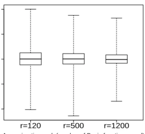
In Figure 5, we show the box plot of the prediction error, for several choices of r. It can be noticed that the prediction quality increases with increasing the number of basis functions. But based on section IV-B, we know that the computational complexity is O(N r2_{) and r << N. As a consequence}

the choice of the parameter r defines the trade-off between computational complexity and prediction quality. Figure 6 presents the prediction error for different numbers of available measurements, considering the same rankr= 1200. One can see that when the number of available measurements is much

r=120 r=500 r=1200 −20 −10 0 10 20

Approximation rank (number of Basis functions used)

Prediction error (dB)

Fig. 5. Influence of the number of basis functions on the prediction error with a fixed number of observed measurements20000(p= 50%).

higher than r (>= 6000), we do not obtain any additional gain on the prediction quality by increasing the number of measurements. This is due to the fact that fixing the rank by using basis functions with truncated shapes results in decreas-ing the spatial correlation impact. Notice from Figures 5 and

2000 6000 20000 32000 −20 −10 0 10 20 30

Number of measurement points

Prediction error (dB)

Fig. 6. Influence of the number observed of measurements on the prediction error with a fixed number basis functions (r= 1200).

6, that the prediction errors involved in FRK are considerably low (variance in the order of 1-3 dB) when compared to, for example, errors in typical propagation models (RMSE between 10-50 dB) with the exception of ray-tracing models that have substantially high computational complexities [17].

V. CONCLUSION

In this paper we have studied the performance of the Fixed Rank Kriging (FRK) algorithm applied to coverage analysis in cellular networks. This method is attractive when performing prediction using massive data sets (order of thousands and higher) as it offers a good trade-off between prediction quality and computational complexity compared to classical Kriging techniques. We have also adapted the FRK algorithm to the considered radio measurements by introducing the EM

algorithm to estimate the model parameters. To evaluate the performance of our prediction and estimation method, we have analysed the prediction error for different numbers of available measurements and for different values ofr,rbeing the ”rank” corresponding to the number of basis functions used in FRK. We have shown that the choice of r impacts the prediction quality, and that we obtainreasonableprediction errors with a relatively low computational complexity (compared to typical errors obtained by existing propagation models, except ray-tracing models which have very high computational complex-ities). We have also shown that once r is fixed, limited gain is obtained by this technique when we increase the number of measurements. This study has been performed using field-like measurements obtained from an accurate and realistic planning tool which uses a ray-tracing propagation model. The next step of this work consists of applying our algorithm to real field measurements.

REFERENCES

[1] 3GPP TR 36.805 v1.3.0 1, “Study on minimization of drive-tests in next generation networks; (release 9),” tech. rep., 3rd Generation Partnership Project, 2009.

[2] B. A. Fette,Cognitive radio technology (Communications Engineering). Newnes, 2006.

[3] Y. Zhao, B. Le, and J. H. Reed, “Network support-the radio environment map,”Cognitive radio technology, pp. 325–366, 2006.

[4] “Flexible and spectrum aware radio access through measurements and modelling in cognitive radio systems,” Tech. Rep. 73, FARAMIR Deliverable D4.1, 2011.

[5] N. A. Cressie, “Statistics for spatial data,” 1993.

[6] B. Sayrac, A. Galindo-Serrano, S. B. Jemaa, J. Riihij¨arvi, and P. M¨ah¨onen, “Bayesian spatial interpolation as an emerging cognitive radio application for coverage analysis in cellular networks,”Trans on Emerging Telecommunications Technologies, 2013.

[7] S. Grimoud, B. Sayrac, S. Ben Jemaa, and E. Moulines, “Best sensor selection for an iterative rem construction,” inVTC Fall, pp. 1–5, IEEE, 2011.

[8] B. Sayrac, J. Riihij¨arvi, P. M¨ah¨onen, S. Ben Jemaa, E. Moulines, and S. Grimoud, “Improving coverage estimation for cellular networks with spatial bayesian prediction based on measurements,” in SIGCOMM, pp. 43–48, 2012.

[9] S. Grimoud, S. Ben Jemaa, B. Sayrac, and E. Moulines, “A rem enabled soft frequency reuse scheme,” inGLOBECOM Workshops, pp. 819–823, 2010.

[10] N. Cressie and G. Johannesson, “Fixed rank kriging for very large spatial data sets,” Journal of the Royal Statistical Society: Series B (Statistical Methodology), vol. 70, no. 1, pp. 209–226, 2008. [11] M. Katzfuss and N. Cressie, “Tutorial on fixed rank kriging (frk) of

co2 data,” 2011.

[12] J. M. Geoffrey and K. Thriyambakam,The EM algorithm and exten-sions, vol. 382. Wiley-Interscience, 2007.

[13] J. Jacod, P. Protter, et al., L’essentiel en th´eorie des probabilit´es. Cassini, 2003.

[14] H. V. Henderson and S. R. Searle, “On deriving the inverse of a sum of matrices,”Siam Review, vol. 23, no. 1, pp. 53–60, 1981.

[15] M. Gudmundson, “Correlation model for shadow fading in mobile radio systems,”Electronics letters, vol. 27, no. 23, pp. 2145–2146, 1991. [16] “Asset tool.” http://www.aircominternational.com/Products/Planning/

asset.aspx.

[17] C. Phillips, D. Sicker, and D. Grunwald, “Bounding the error of path loss models,” inDySPAN, pp. 71–82, 2011.

[18] P. Billingsley,Probability and measure, vol. 939. Wiley, 2012. [19] G. A. Seber and A. J. Lee,Linear regression analysis, vol. 936. John

[20] A. Galindo-Serrano, B. Sayrac, S. Ben Jemaa, J. Riihijarvi, and P. Ma-honen, “Automated coverage hole detection for cellular networks using radio environment maps,” inWiOpt, pp. 35–40, 2013.

[21] T. Cai, J. van de Beek, B. Sayrac, S. Grimoud, J. Nasreddine, J. Riihi-jarvi, and P. Mahonen, “Design of layered radio environment maps for ran optimization in heterogeneous lte systems,” inPIMRC, pp. 172–176, 2011.

[22] K. B. Petersen, M. S. Pedersen, J. Larsen, K. Strimmer, L. Christiansen, K. Hansen, L. He, L. Thibaut, M. Baro, S. Hattinger, V. Sima, and W. The, “The matrix cookbook,” tech. rep., 2006.

APPENDIXA ESTEP Our model is

Y =T α+Sη+ε,

where η andε play the role of random-effect process. Since

η andεare two independent process, we have

Y|η,θ∼N T α+Sη, σ2Ξ

. (24)

In addition,

η|θ∼N (0,K), (25)

where θ = [α, σ2, φ, β]T and the matrix K is defined in equation (16). Then, the EM Q-function is written as

Q(θ,θ(l)) =EY|θ_(l)[ln Pr(Y,η|θ)],

=EY|θ(l)[ln(Pr(Y|η,θ) Pr(η|θ))], (26)

where under the expectationEY|θ_(l), the distribution ofη is a

Gaussian distribution with mean and covariance matrix given in appendix C. Using (24) and (25), we have

EY|θ(l)[ln Pr(Y|η,θ)] (27) =−n 2ln(2πσ 2₎₋ 1 2σ2EY|θ(l) h kY −T α−Sηk2i and EY|θ(l)[Pr(η|θ)] (28) =−r 2ln(2π)− 1 2ln(det(K))− 1 2EY|θ(l) ηTK−1η

Combining (27) and (28) in expression (26) gives

Q(θ,θ(l)) =− n 2 ln(σ 2₎₋ 1 2σ2EY|θ(l) h kY −T α−Sηk2i −1 2ln(det(K))− 1 2EY|θ(l) ηTK−1η +c, (29) wherecis a constant, independent ofθ. Developing the square term in expression (29), we get:

Q(θ,θ(l)) =−n 2 ln(σ 2 )−1 2ln(det(K))− 1 2σ2kY −T αk 2 + 1 σ2(Y −T α) T_S EY|θ(l)[η] −1 2EY|θ(l) " ηT(S T_S σ2 +K −1_)η # +c.

We introduce one of the matrix expectation properties (See [19]), E h XTAXi= Tr(A_E (X−E[X])(X−E[X])T) +E[X]TAE[X], (30)

assuming that Ais a symmetric matrix and X is a vector of random variables. Applying this property, equation (26) takes the form: Q(θ,θ(l)) =−n 2 ln(σ 2₎₋1 2ln(det(K))− 1 2σ2kY −T αk 2 −1 2Tr ( STS σ2 +K −1₎ EY|θ(l) ηηT ! + 1 σ2(Y −T α) T_S EY|θ_(l)[η]. (31) APPENDIXB M-STEP

In the M step, we need to compute the updateθ(l+1)which

is under the following constraint,

Q(θ(l+1),θ(l))>Q(θ(l),θ(l)). (32)

Thenθ(l+1)can be any value that increasesQ(θ,θ(l)). If the

maximum ofQ(θ,θ(l))has a close form the update ofθ(l+1)

can be given by

θ(l+1)= argmax

θ

Q(θ,θ(l)). (33)

To maximizeθ7→Q(θ,θ(l)), we can maximize terms

contain-ing each parameter (α,σ2_{,K). In fact, we start by computing}

first derivative with respect to each parameter independently and then set the obtained derivation equation to zero. The solution of this equation can be a minimum, a maximum, or an inflection point. Therefore, we proceed by computing the second order derivative with respect to the given parameter evaluated for the obtained solution and check that gives a negative number.

a) Updateα: Deriving equation (31) with respect toα

gives ∂αQ(θ,θ(l)) = 1 σ2T T_(Y −T α)− 1 σ2T T_S EY|θ(l)[η]. (34)

We can easily computeαnewwhich is the solution the equation

(34) setted equal to zero. It is given by,

αnew= TTT −1 TTY −S_EY|θ(l)[η] . (35)

To ensure that the solution of∂αQ(θ,θ(l)) = 0is a maximum,

we compute the second order derivative of Q(θ,θ(l)) with respect to α and check it is negative. This gives

∂_α2Q(θ,θ(l)) _θ=(α new,σ2,K)=− 1 σ2T T_{T <0, ∀σ}2_,∀K

As consequence, the computed update αnew satisfies the M-step condition, written as

b) updateσ2_{: To find the update ofσ}2_{, we derive the}

equation (31) with respect toσ2_{, we get:}

∂σ2Q(θ,θ(l)) (37) =− n 2σ2 + 1 2(σ2₎2Tr STS_EY|θ(l) ηηT + 1 2(σ2₎2kY −T αk 2 − 1 (σ2₎2(Y −T α) T_S EY|θ(l)[η].

Setting it equal to zero, we obtain

σ_new2 = 1 nkY −T αnewk 2 + 1 nTr(S T_S EY|θ(l) ηηT ) − 2 n(Y −T αnew) T_S EY|θ(l)[η]. (38)

Sinceσ2is a positive number, we need to check thatσ2new>0.

Therefore, we re-arrange the terms in equation (38) based on the property introduced in (30), we get

σ2new= 1 nEY|θ(l) h kY −T αnew−Sηk2i_>0 and ∂_σ22Q(θ,θ(l)) _θ=(α new,σ2new,K) =− n 2(σ2 new)2 <0. (39) Thenσ2

newsatisfies the M-step assumption, which is,∀σ2,K Q(αnew, σ2_new,K;θ(l))>Q(αnew, σ2,K;θ(l)). (40)

c) Updateβ: Based on the definition of the matrixK

introduced in equation (16), we denote K = 1_βK˜(φ). We derive (31) with respect to β, it gives

∂βQ(θ,θ(l)) = 1 2 r β − 1 2Tr ˜ K(φ)−1EY|θ(l) ηηT (41) Setting this derivative equal to zero, we compute the update of β. It is given by, βnew= r TrK˜(φ)−1 EY|θ(l)[ηη T_] , = r EY|θ(l) h ηT_K˜_(φ)−1_ηi >0 (42) where, ∂2_βQ(θ,θ(l)) _{θ=(α,σ2,β} new,φ)=− r β2 new <0 (43)

Considering αnew and σ2new computed before, we obtain:

∀φ, β

Q(αnew, σnew2 , βnew, φ;θ(l))>Q(αnew, σnew2 , β, φ;θ(l)).

(44) d) Update φ: We notice that when deriving equation (31) with respect to φ, we get a complicated expression with no explicit solution when setted equal to zero. In such a case when no closed form exists it may be feasible to attempt to find the value φ that globally maximizes the function Q(θ,θ(l)).

This case is defined as the generalized EM algorithm (GEM), for which the M-step requires only that φ(l+1) satisfies Q(α, σ2, β, φ(l+1);θ(l))>Q(α, σ2, β, φ(l),θ(l)),∀α∀β,∀σ2.

(45)

In this situation, where we don’t have a closed form for updating parameter φ, we can use one step of the Newton-Raphson (NR) method [12], as the M-step. This gives

φ(l+1)=φ(l)−a(l) ∂φQ(θ,θ(l)) θ=α(l+1),σ₍2_l+1),β(l+1),φ(l) ∂2 φQ(θ,θ(l)) _θ= α(l+1),σ(2l+1),β(l+1),φ(l) , (46) where0< a(l)61. This parameter controls the convergence

rate, we can choosea(l)= 1. We compute derivatives involved

in equation (46) based on some results from matrix derivation theory detailed in [22] and we get

∂φQ(θ,θ(l)) =− 1 2Tr K−1∂K ∂φ (47) +1 2Tr K−1∂K ∂φK −1 EY|θ(l) ηηT , ∂_φ2Q(θ,θ(l)) = 1 2Tr K−1∂ 2_K ∂2_φ(K −1 EY|θ(l) ηηT −Idr) +1 2Tr K−1∂K ∂φK −1∂K ∂φ(Idr−2K −1 EY|θ(l) ηηT ) .

Finally the derivatives of Kwith respect to φare defines as,

_∂K ∂φ i,j = _{∂K(β, φ)} ∂φ i,j = ksi−sjk 2 exp(φ) Ki,j and _∂2_K ∂2_φ i,j =− _{∂K(β, φ)} ∂φ i,j +ksi−sjk 2 exp(φ) _{∂K(β, φ)} ∂φ i,j . APPENDIXC CHARACTERIZATION OFη

We want to identify the conditional distribution ofη given

Y when the value of the parameter is θ, it is denoted by Pr (η|Y,θ). We have,

Pr (η|Y,θ) = Pr (Y|η,θ) Pr (η|θ) Pr (Y|θ) .

Using expression (24) and (25) and up to a multivariate constant independent ofη, we can write:

Pr (η|Y,θ)∝exp(− 1 2σ2kY −T α−Sηk 2 ) (48) ×exp(−1 2η T_K−1 η) ∝exp ₁ σ2(Y −T α) T_{Sη (49)} −1 2η T₍SS t σ2 +K −1_)η ,

We observe that η 7→Pr (η|Y,θ) follows a Gaussian distri-bution with mean µand covariance matrix C. We have

Pr (η|Y,θ)∝exp −1 2(η−µ) T_C−1 (η−µ) , ∝exp −µTC−1η−1 2η T_C−1 η . (50)

Using (48) and (50), we can identify the mean and the covariance ofη|Y,θ: ( µ=EY|θ[η] = (S T S+σ2K−1)−1ST(Y −T α), C=_EY|θ (η−µ)(η−µ)T = (S_σT2S +K −1₎−1_, which yields, EY|θ ηηT = (S T_S σ2 +K −1₎−1_+µµT_. (51)