The median voter hypothesis, income inequality and income
redistribution: An empirical test with the required data
Branko Milanovic*
World Bank, Development Research Group, Washington D.C. 20433 USA Received June 1999, revised December 1999, accepted January 2000 Abstract
The median voter hypothesis has been central to an extensive literature on consequences of income distribution. For example, it has been proposed that greater
inequality is associated with lower growth, because of the greater redistribution that is sought by the median voter when income distribution is less equal. There have however been no proper tests of the median-voter hypothesis concerning redistribution, because of previous absence of data on factor income distribution (that is, incomes before taxes and transfers) across households, and thus on the gains by poorer households from redistribution. The study reported in this paper is based on the required data, with 79 observations drawn from household budget surveys from 24 democracies. The results strongly support the conclusion that countries with greater inequality of factor income redistribute more to the poor. This is so even when we control for the share of the elderly in the population and for pension transfers. The evidence that the median-voter hypothesis adequately describes the collective-choice mechanism is however considerably weaker. Although middle-income groups gain more/or lose less through redistribution in countries where initial (factor) income distribution is more unequal, this regularity is all but lost when, by excluding pensions, we look only at explicit redistributive social transfers fromwhich the middle classes contemporaneously gain little.This leaves us searching for alternative explanations: do middle-classes gain from transfers in the long-run even if not contemporeneously?, or is the median voter hypothesis, based on direct democracy, a proper representation of the the mechanisms of collective-decision making in representative democracy?
JEL classification: D31, E62
Keywords: median voter; income distribution, income inequality
1. Setting the problem: the link between inequality and redistribution
A key relationship in the literature on inequality and growth (see Perotti 1992; Perotti 1993; Persson and Tabellini 1991; Bertola 1993; Alesina and Rodrik 1994; Alesina and Perotti 1994) concerns the link between market-generated income inequality and the extent of redistribution. In Perotti’s (1996, pp. 151) extensive empirical review of the theories linking growth, income distribution, and democracy, this relationship appears under the title of an “endogenous fiscal policy approach.” This approach includes two components or structural equations. The first component is a political mechanism through which greater income inequality leads to greater redistribution and thus more distortionary taxation. The second component is an economic mechanism through which the distortionary taxation reduces growth. The conclusion is that greater income inequality slows growth. In this paper I will be concerned only with the first of these components involving the political mechanism. This mechanism is based on the median-voter hypothesis of income redistribution.
When individuals are ordered according to their factor (or market) incomes,1the median voter (the individual with the median level of income) will be, in more unequal societies, relatively poorer. His or her income will be lower in relation to mean income. If net transfers (government cash transfers minus direct taxes) are progressive, the more unequal is income distribution, the more the median voter has to gain through joint of taxes and transfers, and the more likely he or she is to vote for higher taxes and transfers.2 Based on the median-voter as decisive, more unequal societies will therefore choose greater redistribution.
This approach assumes that (1) voters’ decisions on transfers and taxes are determined solely by their position in the income distribution, (2) preferences of voters are single-peaked, and (3) all (or almost all) individual vote.
The last assumption implies that the relationship between market-generated
inequality and redistribution should be more pronounced in democracies than in authoritarian regimes where governments can decide to ignore the preferences of the poor (see Perotti 1996, p. 171; Alesina and Perotti, 1994; Alesina and Rodrik, 1994, p. 478).
1
Factor income is income before government fiscal redistribution (via cash social transfers and personal income taxes). Factor (i.e. market) income includes wages and bonuses, property income, self-employment incomes, gifts and remittances, home consumption, etc. I will use the terms “factor” and “market” income interchangeably
2
As Alesina and Perotti (1994, p. 360) observe: “in the fiscal channel [explanation], the level of government expenditure and taxation is the result of a voting process in which income is a main determinant of a voter’s preferences: in particular, poor voters will favor high taxation.”
Previous research has not included a structural equation for the underlying median-voter political redistribution mechanism. What researchers have done in their empirical analysis is to estimate the reduced form equation in which inequality in distribution of
disposable income is used as a regressor to explain the growth rate over a period of time (see
Persson and Tabellini 1991; Alesina and Rodrik, 1994; Alesina and Perotti 1994; Easterly and Rebelo, 1993). They do this because the data required to estimate the structural equation are difficult to obtain: factor income distribution was, until recently, unavailable, and, without data on factor income distribution, one cannot calculate the extent of redistribution.
Thus, neither the extent of redistribution nor the mechanism by which it occurs—the median voter hypothesis—has been tested directly.
There are, however, qualifications to this observation. Perotti (1993 and 1996), Easterly and Rebelo (1993, p. 436), and Bassett, Burkett and Putterman (1999) estimate a structural equation of the type
(1) T = f(Id,Z)
where T denotes taxes or social transfers as a share of GDP, or as in Perotti (1996) the marginal tax rate. Id is an index of inequality of disposable income, and Z denotes other relevant variables (e.g., a democracy dummy variable, or percent of population over 65 years of age, since a larger share should imply greater transfers for pensions). Perotti’s 1996 paper presents the most detailed test. He finds lack of a significant relationship between the equality variable (“middle class share” defined as the combined income shares of the third and fourth quintiles of the population ranked according to disposable income) and the marginal tax rate in various formulations: this is so whether the share of the middle class alone is included in the equation, or is interacted with a democracy dummy. Even in a sample of democracies alone, the coefficient has the right sign but is not significant (Perotti, 1996, Table 8, p. 170). When, instead of the marginal tax rate, Perotti uses, on the left-hand side, social security and welfare, or health and housing, or education expenditures (each as a share of GDP), greater inequality in disposable income is associated with greater social transfers only in the case of democracies, and for social security and welfare alone. Perotti concludes (p. 172) that
“…there is .. very little evidence of a negative association between equality and fiscal variables in democracies. It is true that in the political mechanism, [the variable that interacts the share of the middle class and democracy] has the expected negative sign in four cases out
of six, but social security and welfare is the only type of expenditure for which it is significant.”
Bassett, Burkett and Putterman (1999) re-estimated these relationships using three redistribution proxies, (i) public transfers, (ii) social security transfers, and (iii) social security and education as share of GDP), and the share of the middle quintiles in disposable income as the inequality proxy. They too find that the coefficient on the median voter either has a “wrong” sign (a higher share of the middle class increases transfers) or is not
statistically significant. Moreover, their results are highly unstable.
Thus, in the only two direct empirical tests of the median voter hypothesis, the hypothesis is found wanting.
The above approach is however doubly unfortunate, since both the left-hand side and the right-hand side variables are misspecified. On the right-hand side, there is disposable income inequality, which is inequality after both taxes and transfers. However, people’s voting decisions about redistribution are based on their incomes before redistribution.3 It is methodologically incorrect to explain people’s decisions about their personally optimal level of taxes and transfers as depending on the distribution that emerges as a consequence of these decisions.
The approach thus has a time-sequencing problem. In reality, people first receive their factor incomes, and then decide how much they are willing to redistribute through taxation and social transfers. The methodologically correct approach is to specify the decision regarding the extent of redistribution as depending on the distribution of market or
factor (pre-transfer and pre-tax) incomes.
It is also incorrect to use as the dependent variable the share of government transfers in GDP or the marginal tax rate. It is not the share of GDP that matters here, but a measure of the extent of redistribution through transfers and taxes. A society with high taxes and transfers may have contributors and beneficiaries who are the same people. Looking at the share of transfers or taxes in GDP would then give the mistaken impression that the society has chosen substantial redistribution when the reality is exactly the opposite and
redistribution is minimal. Corporatist societies of continental Europe (Austria, Germany) are often considered to follow predominantly such policies (see Esping-Andersen 1990). Le
3
For example, Alesina and Rodrik (1994) are aware of that, because they model a person’s decision on the level of taxation on his capital/labor income ratio, that is, on his factor incomes.
Grand (1982) has similarly proposed that most transfers are given to the middle class. The essential point is that the size of transfers is in itself an imperfect indicator of the extent of redistribution. A correct approach investigates how much the bottom groups in the population according to factor income increase their share in disposable income as a consequence of redistribution. That is, a correct approach estimates the income gain of the poor.
The relationship that we should test is (2) R= f(Im,Z)
where R is an index of redistribution and Im is an index of inequality of factor incomes. Equation (2) specifies the extent of redistribution as a function of the initial inequality with which factor incomes are distributed.
This formulation is flexible. Voters may choose small but very redistributive polices or a series of extensive, but less redistributive, programs. Each type of policy may reduce initial inequality equally.
There are two hypotheses present here. The first hypothesis is that countries with more unequal initial incomes redistribute more. The second hypothesis proposes one explanation for why this may be so—the median voter hypothesis. These are two distinct hypotheses. The first is purely empirical. The second is about a specific political mechanism.
Observe both sides of the correct specification (2) differ from (1). This is because both sides of (1) are proxies for the “true” variables: the share of transfers in GDP or the marginal tax rate is a proxy for redistribution; and inequality in distribution of disposable income is a proxy for inequality in distribution of factor income.
As I have noted, previous researchers have used equation (1) rather than (2) because the information on factor income inequality indispensable for both sides of equations (2) has for most countries been unavailable. The income distribution statistics that have been available have, almost without exception, indicated disposable or gross (market plus
transfers) income. It is only recently that the Luxembourg Income Survey (LIS) database has provided factor income distributions for a number of countries.
The LIS data enable us to observe changes in income distribution in the transition from pure market-determined incomes to incomes that include government cash transfers (gross income), and finally in the transition to disposable income (gross income minus direct personal taxes).
Moreover, since almost all countries in the LIS database are democracies, the two hypotheses can be tested precisely for the countries with the democratic institutions that are assumed to be present when appealing to the median-voter hypothesis.
The paper is organized as follows. Section 2 describes the database. Section 3 considers the relationship between factor income inequality and redistribution. Section 4 tests the median voter hypothesis. Section 5 concludes the paper.
2. Description of the database
I use data for 24 countries that were, with two exceptions, democracies at the time of the surveys.4 Most of the countries were long-established democracies—with at least 20 years of uninterrupted democracy prior to the survey. Several had only a few years of democracy prior to the survey (e.g. Spain in 1980, Russia in 1992, the Czech republic and Slovakia in 1992, Hungary in 1991, Taiwan in 1991). We define as established democracies (EDs) all countries with exception of transition countries (Russia, Czech republic, Slovakia, Poland, and Hungary), and Taiwan.
The Luxembourg Income Survey (LIS) standardizes countries’ own household income surveys5by making the definitions of variables (e.g. pension income, factor income, remittances etc.) as similar as possible. LIS is the only such source of standardized
individual unit record data for developed market economies. I have used all the data that LIS had as of fall 1999.6 There are altogether 79 country observations. For each observation, we have the average per capita income in local currency by decile for the following six
distributions:
4
The exceptions are Poland in 1986 and Taiwan in 1981 and 1986. The following country data sets are included: Australia 1981, 1985, 1989, and 1994; Belgium 1985, 1988 and 1992; Canada 1975, 1987, 1991 and 1994; Czech Republic 1992; Denmark 1987 and 1992; Finland 1987, 1991 and 1995; France 1979, 1981, 1984 and 1989; West Germany 1973, 1978, 1981, 1984, 1989 and 1994; Hungary 1991; Ireland 1987; Israel 1979, 1986 and 1992; Italy 1986, 1991 and 1995; Luxembourg 1985, 1991 and 1994; the Netherlands 1983, 1987, 1991 and 1994; Norway 1986, 1991 and 1995; Poland 1986, 1992, and 1995; Taiwan (Province of China) 1981, 1986, 1991 and 1995; Russia 1992 and 1995; Slovakia 1992; Spain 1980 and 1990; Sweden 1967, 1975, 1981, 1987, 1992 and 1995; Switzerland 1982; United Kingdom 1969, 1974, 1979, 1986, 1991 and 1995; United States 1974, 1979, 1986, 1991, 1994 and 1997.
5
The list of the exact individual country surveys used by LIS to generate its database can be found at the website http://dpls.dacc.wisc.edu/apdu/lis_chart.html.
6
There are four “waves” of data: from mid-1970’s and early 1980’s; from the second half of the 1980’s; from the late 1980’s and early 1990’s; and from mid-1990’s up to 1997.
(1) The distribution of factor income (which ranks individuals by household per capita factor income).
(2) The distribution of factor income P, which is equal to factor income (1) plus pension transfers (which ranks individuals by household per capita factor income
P).
(3) The distribution of gross income (which ranks individuals by household per capita gross income).
(4) The distribution of disposable income (which ranks individuals by household per capita disposable income).
(5) The distribution of disposable income (which ranks individuals by household per capita factor income).
(6) The distribution of disposable income (which ranks individuals by household per capita factor income P).
Factor income is defined as pre-transfer and pre-tax income, and includes wages, income from self-employment, income from ownership of physical and financial capital, and gifts.7 Factor income P includes in addition public pensions. This is a factor income definition specially created for this study.
The reason for including pensions along with the usual factor incomes is that pensions are specific transfers that do not respond to current contingencies, and are not paid with the objective of redistributing income. Pensions are, of course, deferred wages, with some redistribution component. By treating pensions as factor income, we can better focus on other social transfers such as unemployment benefits, family allowances, and social
assistance that have a clear redistributive function.
7
The exact definition of factor income, using LIS notation, is as follows. Our factor income is equal to LIS-defined factor income [FI=net wage and salary income (V1) + farm self-employment income (V4) + non-farm self-employment income (V5) + cash property income (V8) ] plus private pensions (V32) plus occupational public pensions (V33) plus alimony received (V34) plus other regular private income (V35) (household transfers) plus other cash income (V36). Factor P income is equal to factor income plus cash social security benefits for old age or survivors (V19).
Gross income is equal to factor income plus all government cash transfers. Disposable income is equal to gross income minus direct personal taxes and mandatory employee contributions.8
For each type of distribution data listed above, we can calculate indicators of inequality as well as indices of redistribution. Tables 1a and 1b show the average Gini coefficients for the four concepts of income (factor, factor P, gross, disposable). Gini coefficients for individual countries are shown in Annex Table 1.
Each concept focuses on a different underlying reason for inequality. Factor income inequality reflects the distribution of human, physical and financial assets as well as the relative prices of these assets. This is the distribution of income in the absence of
government intervention.9 Gross income adjusts only for government cash transfers. Finally, the distribution of disposable income—which is commonly used—shows differences in purchasing power among individuals.
An example demonstrates how the different concepts highlight different aspects of distribution. Consider Sweden and the US in the mid-1990’s. In terms of disposable income inequality, these two countries are very different: the Gini for Sweden is 26, the Gini for the US is much higher – actually the highest among all established democracies— 42.3 (in 1997). Yet, the two countries are almost identical in terms of factor income inequality, or, in other words, in terms of underlying asset distributions. Sweden’s factor income Gini in the 1990’s was 51-52, while the US’s Gini ranged between 50 and 53.
Using the data from (5) and (6) [when income concept and the ranking criterion differ], we can calculate precisely the extent of gain realized by lower income groups through government transfer and tax systems.
8
The exact definitions are as follows. Gross income is equal to factor income plus social insurance transfers (sick pay, disability pay, social retirement benefits, child or family allowances, maternity pay, military or veterans benefits, and other social insurance) plus social assistance transfers (means-tested cash benefits and near-cash benefits). Gross income minus mandatory employee contributions minus income tax equals disposable income. See the Luxembourg Income Study variable definitions in http://lissy.ceps.lu.summary.htm.
9
This is simplification, because, if the government were truly absent, there would be, for example, more private pensions, and the factor distribution would be different.
Table 1a. Inequality: descriptive statistics for all countries Mean Standard
deviation
Maximum (country) Minimum (country)
(1) Factor income Gini 46.3 5.8 62.0 (Russia 95) 31.4 (Taiwan 86) (2) Factor income P Gini 39.8 5.6 53.2 (Ireland 87) 30.0 (Czech 92) (3) Gross income Gini 38.5 6.7 56.4 (Russia 1995) 24.8 (Slovakia 1992) (4) Disposable income Gini 32.2 5.3 48.8 (Russia 1995) 20.9 (Slovakia 1992) Reduction of inequality (1)-(4) 14.1 5.3 24.9 (Sweden 1992) -0.5 (Taiwan 1981) Reduction of inequality (2)-(4) 7.6 3.7 15.5 (Ireland 87) 0.3 (Italy 86)
Table 1b. Inequality: descriptive statistics for established democracies Mean Standard
deviation
Maximum (country) Minimum (country)
(1) Factor income Gini 46.6 4.2 55.8 (Ireland 87) 36.4 (Finland 87) (2) Factor income P Gini 40.2 5.0 53.2 (Ireland 87) 32.2 (Finland 87)
(3) Gross income Gini 36.9 6.1 53.8 (US 97) 28.5 (Belgium 85)
(4) Disposable income Gini 32.1 4.7 42.3 (US 97) 23.3 (Finland 97) Reduction of inequality (1)-(4) 14.5 4.2 24.9 (Sweden 92) 7.1 (Switzerland 81)
Reduction of inequality (2)-(4) 8.1 3.3 15.5 (Ireland 87) 0.3 (Italy 86)
On average, government transfers and taxes reduce factor income inequality by more 14 Gini points (Table 1a and Table 1b). Almost a third of factor-income inequality is thus removed by government. Most of the reduction (7.8 Gini points for the entire sample, or 9.7 Gini points for the established democracies) is achieved through cash transfers. Reductions of respectively 6.3 and 7.8 Gini points are due to direct personal taxes.
It is also apparent that differences among the countries’ Ginis, particularly among the established democracies, are small. This is consistent with expectations for countries that have similar income levels, political systems, and age structure of their populations. The unweighted coefficient of variation of disposable income Gini coefficients is about 0.15— which contrasts with the world coefficient of variation of about 0.35 (see Milanovic, 1999).
Table 1b also shows that, while Ireland has the highest factor income inequality among EDs, it is overtaken by the US as the country with the highest gross and disposable income inequality. At the opposite end of the spectrum, we find Finland –the only West European country with the factor income Gini below 40, and the only one that comes close to Taiwan—and Sweden. Finland and Sweden have disposable income Ginis around 25. For the full sample, Slovakia and the Czech republic have the lowest disposable income Ginis.
Who benefits from redistribution in the move from factor to disposable income? Tables 2a and 2b show the average share gain for each of the bottom five deciles (defined according to their factor incomes). We define the “share gain” as the difference (formed according to factor income) between the share of a given decile in factor and disposable income. For example, if the bottom decile receives 2 percent of total factor income, while the same people receive 8 percent of total disposable income, the share gain is 6 percentage points. The share of the bottom decile (formed according to factor income) increases, on average, by 5.7 percentage points in the entire sample, or by 5.8 percentage points in EDs (going from respectively 0.3 and 0.2 percent of total factor income to 6 percent of disposable income). The persons in the second decile according to factor income gain, on average, 4.0 (the entire sample) or 4.2 (EDs only) percentage points. Their share increases from 1.9 and 1.8 percent of factor income to 5.9 or 6 percent of total disposable income.10 The share gain decreases with level of (factor) income, and becomes practically nil for the fifth decile. The combined poorest 50 percent of people by factor incomes have a share gain of 12.4
percentage points (in the entire sample) or 12.9 percentage points (for EDs only). The people in the upper half of factor income distribution are losers in redistribution.
Tables 3a and 3b are identical to Tables 2a and 2b, except that we now look at the share gain between factor P income and disposable income. The advantage of this measure is that pensions are not treated as a redistribution transfer.
10
Note that the same disposable income share of the people who are in the bottom or the second decile according to factor income shows that, on average, is does not matter whether one is in among the bottom 10 percent or in the second decile according to factor income.
The extent of redistribution is often overestimated when we look at the share gain between factor and disposable income (as in Tables 2a and 2b). Consider the following. For many pensioners, state pensions are often the only, or at least the most important, source of income. According to factor income, pensioners will tend to be ranked in lower—often the lowest—income decile. Once we move from factor to gross and disposable income, their position dramatically improves simply because they have received a significant income source—a pension.11 Everything else being the same, a country with many pensioners (i.e. with an older population) will tend to show much larger redistribution: the share gain will be greater.
If we take the view that pensions are not primarily a redistributive transfer and include pensions together with other factor incomes in factor P income, we can recalculate the share gain as in Tables 3a and 3b. The extent of redistribution is now halved. The share gain goes down from more than 12 percentage points to 6 percentage points for the whole sample, and 6.4 for the EDs. Observe that the average share gain is about halved for the first three deciles, and stays about the same for the fourth decile, but increases for the fifth decile.
11
This is particularly noticeable for the East European countries. There pensioners have scarcely any other source of income than pensions. Factor income shows them to be very poor, and since pensions are relatively high, the sharegains are large. Similarly, factor income Gini is high. But once we include pensions with other factor incomes, the “new poor” are not nearly as poor (factor P Gini goes down a lot), and sharegains are much less.
Table 2a. Redistribution (sharegain) by decile for all countries (from factor to disposable income)
Average gain
Standard deviation
Maximum (country) Minimum (country)
Bottom decile 5.7 2.4 9.9 (Slovakia 92) 0.1 (Taiwan 81 and 86)
Second decile 4.0 2.1 9.0 (Belgium 85)
8.9 (W. Germany 84)
0.1 (Taiwan 81 and 86)
Third decile 1.9 1.4 8.7 (Belgium 85)
5.1 (Sweden 92)
0.1 (Taiwan 81, 86, 91)
Fourth decile 0.7 0.6 2.8 (Sweden 95) -0.3 (Italy 86)
Fifth decile 0.1 0.4 0.8 (Sweden 95) -0.9 (Netherlands 94)
Bottom one-half (cumulative five deciles) 12.4 5.4 27.3 (Belgium 85) 23.5 (Poland 95) 0.3 (Taiwan 81)
Table 2b. Redistribution (sharegain) by decile for established democracies (from factor to disposable income)
Average gain
Standard deviation
Maximum (country) Minimum (country)
Bottom decile 5.8 2.0 9.7 (Luxembourg 1985) 2.9 (Sweden 1967)
Second decile 4.2 2.0 9.0 (Belgium 1985)
8.9 (W. Germany 1984)
1.2 UK (1969)
Third decile 1.9 1.4 8.7 (Belgium 1985)
5.1 (Sweden 1992)
0.2 (Germany 1973)
Fourth decile 0.8 0.6 2.8 (Sweden 1995) -0.3 (Italy 1986)
Fifth decile 0.1 0.4 0.8 (Sweden 1995) -0.9 (Netherlands 1994)
Bottom one-half (cumulative five deciles) 12.9 4.7 27.3 (Belgium 1985) 22.5 (Sweden 1992) 5.7 (Switzerland 1982)
Note: Data for Belgium 88 and 92 show zero or almost zero income for the bottom two deciles according to factor income. If these zeros are inaccurate, redistribution may be overestimated. This is why a maximum redistribution country other than Belgium is shown as well.
Table 3a. Redistribution (sharegain) by decile for all countries (from factor P income to disposable income)
Average gain
Standard deviation
Maximum (country) Minimum (country)
Bottom decile 2.8 1.8 7.8 (Spain 80) 0.1 (Taiwan 81)
Second decile 1.4 0.9 4.5 (Norway 79) 0.1 (Taiwan 81)
Third decile 0.9 0.5 2.3 (Sweden 95) 0.0 (Italy 86)
Fourth decile 0.6 0.4 1.4 (Sweden 95) -0.2 (Germany 73)
Fifth decile 0.3 0.3 0.9 (Sweden 81) -0.5 (Spain 80)
Bottom one-half (cumulative five deciles)
6.0 3.1 12.7 (Norway 79) 0.3 (Taiwan 81)
Table 3b. Redistribution (sharegain) by decile for established democracies (using factor P and disposable income)
Average gain
Standard deviation
Maximum (country) Minimum (country)
Bottom decile 3.0 1.7 7.8 (Spain 80) 0.5 (Italy 86)
Second decile 1.5 0.9 4.5 (Norway 79) 0.1 (Italy 86)
Third decile 0.9 0.5 2.3 (Sweden 95) 0.0 (Italy 86)
Fourth decile 0.6 0.4 1.4 (Sweden 95) -0.2 (Germany 73)
Fifth decile 0.3 0.3 0.9 (Sweden 81) -0.5 (Spain 80)
Bottom one-half (cumulative five deciles)
6.4 2.8 12.7 (Norway 79) 0.7 (Italy 86)
Note: Deciles formed according to household per capita factor (or factor P) income. The increase in the share shows the difference between the factor income share of people who are in the bottom (second, third etc.) decile according to factor or factor P income and their share in disposable income.
Table 4 shows the extent of redistribution by country measured by the increase in the share of the persons who are in the bottom quintile and bottom half of the factor income distribution. For simplicity, we shall refer to the bottom 20 and 50 percent of the population
ranked according to factor income as respectively “the very poor”, and “the poor”.
The countries are ranked by the gain in the share of the bottom half. Belgium 85 and 88, and Poland 95 show the largest redistribution both to the lowest quintile and lowest half of the population.12In Poland, pensions, which have increased compared to wages since the beginning of transition, are the principal reason for the extensive redistribution.13
As expected, Sweden, Germany and France have extensive redistribution, with the bottom half gaining between 18 and 22½ percentage points (between 1 and almost 2 standard deviations above the mean), and the bottom quintile gaining between 14 and 17 percentage points (more than 1 standard deviation above the mean).
Redistribution is the smallest in Taiwan, Switzerland, UK in the 1970’s, and the US. In the US 97, for example, the bottom half gains about 8 percentage points (almost 1 standard deviation less than the mean); in Switzerland 82, 5.7 percentage points (almost 1½ below the mean).
The table shows the unique position of Taiwan. This is of particular interest, since Taiwan is the only non-Western country in the sample.14 Taiwan has by far the lowest factor income inequality, a Gini of 31 as against the mean sample Gini of 46. But, perhaps
precisely because factor-income inequality is low, redistribution is nil. Neither the poor nor the very poor gain practically anything in their disposable income share (the bottom half gains between 0.3 and 1.4 percentage points).
The complete data on shares and gains by decile and by country are given in Annex Tables 2 and 3.
Table 5 shows the gain through redistribution when factor income is defined to include pension transfers. Both the extent of redistribution and the rankings of recipients
12
For the reasons mentioned above (Table 2a), the Belgian data may exaggerate the extent of redistribution.
13
This can be seen from Table 5 where the rankings are based on redistribution from factor P income: Poland 95 slips from the second most redistributionist position to the seventh.
14
The “non -Western” means non-European, or of non-European settlement (like Australia, Canada or the U.S.).
change. The most redistributive are the Nordic countries: among the top five countries, four are Nordic; among the top ten countries, six are Nordic.15
Also, once we eliminate pensions, the ranking of countries that have large transfers (most of which are often pensions) such as Germany, Italy and France, and which appear very strongly redistributionist according to factor income (Table 4), slip significantly. In Germany in the 1980’s, the poorest quintile gained only 3 to 4 percentage points as against 14-17 percentage points when calculations are made according to factor income. Italy is shown to be among the least redistributionist countries: the bottom quintile and the bottom half gain between 1 and 2 percentage points, even though according to factor income Italy is more redistributionist than average.
The data in Tables 4 and 5 allow us also to observe how redistribution in individual countries has evolved through time. To illustrate, we look in Figure 1 at four countries, and focus on the most redistributionist measure: share gain of the bottom quintile using the factor P income. We see that, while during the Thatcher period, social transfers in the UK declined as a percentage of GDP, but the share gain of the very poor improved significantly. The same outcome is shown in the case in Sweden and Canada, but not the United States, where the share gain of the very poor in 1997 was the same as quarter of a century previously, and was far smaller than in the other three countries.
15
Although the concept of transfers is narrower in Table 5 than in Table 4, the sharegain (for any given data point) need not be smaller. This is because the ranking of recipients changes and these new recipients (that constitute the bottom quintile or half of the distribution) can be poorer and their gain can be greater even if the concept of transfers is more limited.
Figure 1. Sharegain of the very poor, mid-1970’s-mid-1990’s (using factor P income) 0.0 2.0 4.0 6.0 8.0 1969 1974 1981 1986 1991 1995 1 997 Y ears U S C an ada S w eden U K
Table 4. Redistributional gain of the bottom quintile and bottom half of factor income distribution (in percentage points of disposable income)
Country (year) Gain of the bottom quintile Gain of the bottom half
Belgium 85 17.86 27.32 Poland 95 17.04 23.52 Belgium 88 17.15 22.88 Sweden 92 14.44 22.50 Sweden 95 13.43 21.74 Sweden 81 15.69 21.16 Sweden 87 15.55 20.44 Belgium 92 13.74 19.49 France 89 14.99 19.37 France 84 14.24 18.90 Germany 84 16.90 18.07 Slovakia 92 14.08 17.91 Germany 94 14.37 17.90 Hungary 91 12.31 17.83 Denmark 92 12.52 17.46 France 84 13.72 17.28 Czech republic 92 14.64 17.22 Denmark 87 13.72 17.05 Netherlands 87 13.87 17.05 Sweden 75 13.06 16.55 Netherlands 83 12.58 16.39 Germany 89 14.36 16.03 Luxembourg 94 14.25 15.53 UK 86 10.30 15.27 France 79 12.59 15.23 Germany 81 13.06 14.55
Italy 95 12.70 14.53 Ireland 87 9.72 14.35 Norway 95 10.73 14.27 Luxembourg 85 13.47 13.82 UK 95 8.78 13.73 Luxembourg 91 13.25 13.57 Italy 86 13.22 13.08 Italy 91 12.62 13.04 Finland 95 8.50 12.90 Norway 79 11.47 12.73 Norway 91 9.93 12.58 Poland 92 11.13 12.50 Netherlands 91 10.26 12.46 Spain 90 11.46 12.45 Germany 83 10.46 11.84 UK 91 8.24 11.78 Germany 78 10.87 11.76 Norway 86 10.19 11.35 UK 79 9.31 11.22 Australia 94 8.25 11.13 Canada 94 7.81 11.09 Russia 95 7.24 11.02 Netherlands 94 10.63 10.92 Sweden 67 7.60 10.90 Canada 91 7.07 10.01 Finland 87 7.00 9.94 Israel 92 6.21 9.69 Israel 86 6.01 9.65 Finland 91 6.60 9.64
Spain 80 9.62 9.62 Australia 89 7.66 9.60 Australia 85 7.45 9.41 Poland 86 9.86 9.33 Australia 81 7.58 9.02 US 94 5.39 8.60 Germany 73 8.76 8.44 US 91 5.33 8.43 Canada 87 6.24 8.41 Russia 92 6.43 8.28 US 97 5.25 8.18 Israel 79 5.28 8.11 US 79 5.34 8.06 US 86 4.97 7.56 US 74 5.44 7.06 Canada 81 5.13 6.75 UK 69 5.76 6.74 Canada 75 4.97 6.67 UK 74 5.36 6.27 France 81 4.58 6.00 Switzerland 82 5.24 5.70 Taiwan 95 0.92 1.37 Taiwan 91 0.42 0.65 Taiwan 86 0.23 0.43 Taiwan 81 0.16 0.34 Average 9.75 12.44 Standard deviation 4.19 5.39
Table 5. Redistributional gain of the bottom quintile and bottom half of factor P income distribution (in percentage points of disposable income)
Country (year) Gain of the bottom quintile Gain of the bottom half
Norway 79 11.47 12.73 Denmark 87 10.26 12.35 Sweden 95 7.77 11.89 Denmark 92 8.74 11.88 Ireland 87 8.01 11.77 Netherlands 86 10.19 11.35 Poland 95 8.07 10.64 Netherlands 87 9.10 10.58 Finland 95 6.76 10.56 UK 86 6.70 9.96 Spain 80 9.62 9.62 Sweden 92 6.76 9.58 UK 95 6.77 9.46 Sweden 81 5.47 9.11 Netherlands 83 7.34 8.86 Belgium 92 5.79 8.79 Sweden 75 4.77 8.37 Australia 94 5.89 8.31 Germany 73 8.56 8.30 Slovakia 92 5.83 8.10
Sweden 87 4.81 7.78 UK 91 5.49 7.55 Israel 92 4.60 7.42 Norway 95 5.51 7.40 Hungary 91 4.88 7.32 Finland 91 4.48 7.26 Australia 89 5.10 7.08 Finland 87 4.23 7.07 Netherlands 91 6.01 7.01 Israel 86 3.90 6.82 Canada 94 4.42 6.75 UK 79 4.29 6.55 Norway 91 4.54 6.41 Netherlands 94 6.13 6.35 Canada 91 4.12 6.35 Australia 85 4.02 6.24 Czech 92 4.13 6.11 Australia 81 4.19 5.96 France 89 3.80 5.95 Israel 79 3.34 5.94 Belgium 88 5.15 5.90 Germany 94 3.68 5.89 Belgium 85 4.83 5.80
France 84 3.13 5.58 Germany 81 3.69 5.47 France 79 3.01 5.34 Sweden 67 1.99 5.22 Canada 87 3.23 5.16 US 79 2.96 5.08 France 81 3.32 4.90 Germany 89 2.69 4.85 Germany 84 2.74 4.66 US 91 2.47 4.43 US 94 2.36 4.36 Canada 75 2.76 4.29 Canada 81 2.71 4.20 US 97 2.16 4.09 Luxembourg 94 3.21 4.04 US 86 2.13 3.94 Luxembourg 85 3.61 3.84 Germany 83 2.50 3.77 Poland 86 3.47 3.69 UK 69 2.32 3.45 US 74 1.98 3.37 Spain 90 3.07 3.33 Luxembourg 91 2.81 3.23
Germany 78 1.80 3.08 UK 74 1.84 2.93 Switzerland 82 1.28 2.07 Poland 92 1.41 1.97 Italy 95 1.60 1.85 Russia 92 0.79 1.51 Italy 91 1.05 1.16 Russia 95 0.48 0.95 Taiwan 95 0.53 0.78 Italy 86 0.59 0.67 Taiwan 91 0.30 0.54 Taiwan 86 0.21 0.41 Taiwan 81 0.14 0.32 Average 4.25 6.00 Standard deviation 2.57 3.12
3. Testing the redistribution hypothesis
As pointed out in section 1, the relationship that we should test is: (2) R= f(Im,Z)
We shall use two variables to indicate the extent of redistribution: how the share of (i) the bottom half and of (ii) the bottom quintile (ranked by factor income) increases when we move from factor (or factor P) to disposable income—the variables displayed in Tables 3 and 4.16 We denote these variables as respectively sharegain50 and sharegain20.
Our hypothesis throughout is that both gain variables are positively related to factor income inequality (Im). Several variables can be used as indicators of factor income inequality: the Gini coefficient of factor income (Gm); the share of the bottom half
(share50MM); or the share of the bottom quintile (share20MM) where the double suffix MM indicates that we are dealing with (i) the distribution of factor (=market) income and (ii) that the recipients are ranked by their factor (=market) income.
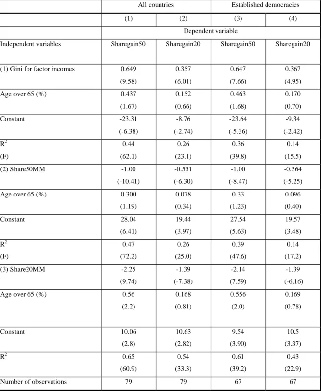
Tables 6a and 6b show the results for the two definitions of factor income. In the version using the standard definition of factor income, we control for the share of population over 65 years of age.17 This is not necessary in the factor P formulation because pensions are included as part of factor P income. Each table combines two indicators of redistribution against three indicators of factor income inequality.
We look first at the full-sample regressions of at Table 6a. The coefficients indicating that greater factor inequality is associated with greater gain of the poor and the very poor, have everywhere the correct sign, and are throughout significant at the 1 percent level. However, the age variable is barely significant in a few formulations, and insignificant in others.
16
Note that gain is defined across the same people. We do not compare the share of the bottom half ranked according to factor income to the bottom half of the distribution ranked according to disposable income.
17
An income control (either as mean dollar income from income surveys or GDP per capita) is statistically insignificant in all formulations.
Consider the expected gain of the poor: each Gini point increase in factor inequality is accompanied by 0.65 percentage point gain of the poor (equation 1.1). If factor income inequality rises by one standard deviation (5.8 Gini points; see Table 1a), the share of the poor in disposable income would, thanks to redistribution, increase by about 3.8 percentage points, e.g. instead of getting 20 percent of disposable income, they would receive 23.8 percent. The share of the very poor would increase by 2.1 percentage points (0.357 from equation 1.2 times 5.9).
The same results are obtained if, instead of the Gini coefficient, we use the share of the bottom half of the population in market income (Share50MM) or Share20MM (see also Figures 2 and 3).The results are even stronger with the factor shares as controls (R2and the t-values are greater).
Table 6a. Redistribution as function of factor inequality (using factor income) fixed effect regresions
All countries Established democracies
(1) (2) (3) (4)
Dependent variable
Independent variables Sharegain50 Sharegain20 Sharegain50 Sharegain20
(1) Gini for factor incomes 0.649 (9.58) 0.357 (6.01) 0.647 (7.66) 0.367 (4.95) Age over 65 (%) 0.437 (1.67) 0.152 (0.66) 0.463 (1.68) 0.170 (0.70) Constant -23.31 (-6.38) -8.76 (-2.74) -23.64 (-5.36) -9.34 (-2.42) R2 (F) 0.44 (62.1) 0.26 (23.1) 0.36 (39.8) 0.14 (15.5) (2) Share50MM -1.00 (-10.41) -0.551 (-6.30) -1.00 (-8.47) -0.564 (-5.25) Age over 65 (%) 0.300 (1.19) 0.078 (0.34) 0.33 (1.23) 0.096 (0.40) Constant 28.04 (6.41) 19.44 (3.97) 27.54 (5.63) 19.57 (3.48) R2 (F) 0.47 (72.2) 0.26 (25.0) 0.39 (47.6) 0.14 (17.2) (3) Share20MM -2.25 (9.74) -1.39 (-7.38) -2.14 (7.59) -1.39 (-6.16) Age over 65 (%) 0.56 (2.2) 0.168 (0.81) 0.556 (2.0) 0.169 (0.78) Constant 10.06 (2.8) 10.63 (2.82) 9.54 (3.90) 10.5 (3.37) R2 0.65 (60.9) 0.54 (33.3) 0.61 (39.2) 0.43 (22.9) Number of observations 79 79 67 67
Note: t-values between brackets. Share50MM=share of total factor income received by the bottom half of the population ranked by factor income. Share20MM=share of total factor income received by the bottom quintile of the population ranked by market income. All R2’s are overall.
Table 6b. Redistribution as function of factor inequality (using factor P income) (fixed effect regresions)
All countries Established democracies
(1) (2) (3) (4)
Dependent variable
Independent variables Sharegain50 Sharegain20 Sharegain50 Sharegain20
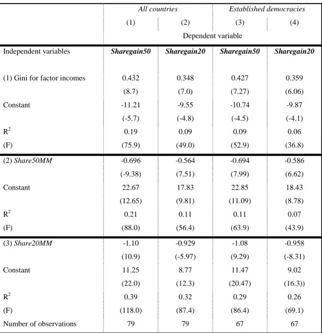
(1) Gini for factor incomes 0.432 (8.7) 0.348 (7.0) 0.427 (7.27) 0.359 (6.06) Constant -11.21 (-5.7) -9.55 (-4.8) -10.74 (-4.5) -9.87 (-4.1) R2 (F) 0.19 (75.9) 0.09 (49.0) 0.09 (52.9) 0.06 (36.8) (2) Share50MM -0.696 (-9.38) -0.564 (7.51) -0.694 (7.99) -0.586 (6.62) Constant 22.67 (12.65) 17.83 (9.81) 22.85 (11.09) 18.43 (8.78) R2 (F) 0.21 (88.0) 0.11 (56.4) 0.11 (63.9) 0.07 (43.9) (3) Share20MM -1.10 (10.9) -0.929 (-5.97) -1.08 (9.29) -0.958 (-8.31) Constant 11.25 (22.0) 8.77 (12.3) 11.47 (20.47) 9.02 (16.3)) R2 (F) 0.39 (118.0) 0.32 (87.4) 0.29 (86.4) 0.26 (69.1) Number of observations 79 79 67 67
Note: t-values between brackets. Share50MM=share of total factor P income received by the bottom half of the population ranked by factor income. Share20MM=share of total factor P income received by the bottom quintile of the population ranked by market income. All R2’s are overall.
For the same equations over the sample of established democracies, we expect to find that the redistributional regularity holds even more strongly. We see that all coefficients again have the right sign and are statistically significant at the 1 percent level. The values of the coefficients hardly change at all.
On average, the gain of the very poor is a little over one-half of the gain of the poor (the coefficient on sharegain20 is between ½ and 0.6 of the coefficient on sharegain50). Equations 2.1 and 2.3 show that a percentage point decrease in the factor-income share of the poor (Share50MM) increases the poor’s share in disposable income by 1 point. The
coefficient of unity indicates that redistribution exactly compensates for the initially lower share of the bottom half of the population. In other words, the poor in a country with a lower factor income share would still end up with exactly the same disposable income share than the poor in a more factor-equal country.
This is not the case for the very poor. The redistribution coefficients in equations 3.2 and 3.4 are throughout greater than 1. For the very poor, in effect, redistribution more than
compensates for their initially lower factor share. Each percent point drop in their factor
income share increases the poor’s share in disposable income by 1.39 percentage points (both in EDs and in full sample). Ironically, the poor are eventually better off if they start worse off!
Table 6b reports the same regressions as in Table 6a except that factor income is now replaced by factor P income. age65 is no longer needed as control variable. The redistribution coefficients again have the right sign and are all highly significant. However, the R2are significantly lower. They increase, though, as we move from equations 1 (factor Gini as control) to equations 3 (share20MM as control). Once pensions are not part of social transfers, the redistribution that we capture reflects transfers directed to the very poor. These transfers therefore offer a superior explanation of the effects on the very poor, as in equation 3. They matter much less for the rest of the population.
The most interesting regressions are 2.1 and 2.3 for the poor, and 3.2 and 3.4 for the very poor. The poor’s gain is now about 70 percent of what it was in earlier regressions when pensions were not part of factor income. For the full sample, the redistribution coefficient goes down, in absolute value, from 1 (equation 2.1 in Table 6a) to 0.696 (equation 2.1 in Table 6b). Similarly, for the very poor, the redistribution coefficient decreases from 1.39 (equation 3.2 in Table 6a) to 0.93 (equations 3.2 in Table 6b).
Clearly, much redistribution simply occurs as result of pension payments. However, there is more to redistribution than that. It is not simply that once pensions are included as part of factor income that total transfers (and redistribution) are less. There is also a re-ranking effect. By not considering pensions as part of factor income, we treat many households who depend on pensions for the large part of their income as poor or very poor. Once pensions are included in factor income, many such households are no longer poor.
Thus, with the factor P definition, not only is redistribution, by definition, less, but both poor and very poor households are different. And transfers shorn of pensions capture much better what happens among the “new poor” (not pensioners).
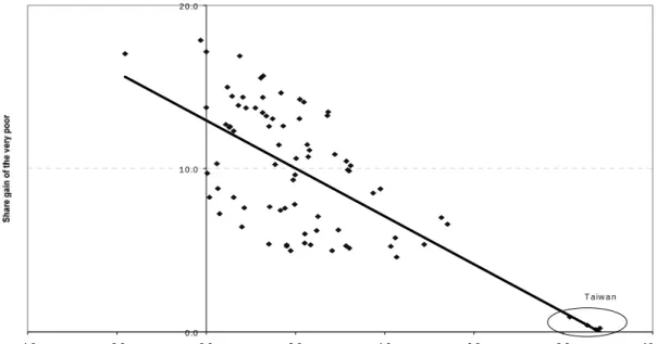
Figure 2. The poors’ gain as function of their share in factor income
Note: Share gain of the poor is the difference between the share of the bottom half of the population in disposable income and factor income. The bottom half of the population are the 50 percent of the people with the lowest per capita factor income.
0.0 10.0 20.0 30.0
5.0 10.0 15.0 20.0 25.0 30.0 35.0
Share of the poor in market income
Taiwan Finland Russia 95 Poland 95 Belgium 85 Belgium 89 Sweden 92 Sweden 95 Switzerland 82 Russia 92 France 91 U.K. 74 Slovak Republic 92
Figure 3. The very poors’ gain as function of their share in factor income
How large is redistribution? We have seen that societies that begin with a more
unequal distribution of factor income are likely to exhibit greater redistribution. The gain is less—although it persists—when we move from the standard definition of factor income to the definition that includes pension transfers.
Now we can ask the question: Will redistribution be so large that the share of the poor will be independent, in terms of disposable income, of their starting position?
Results in Table 7 report the extent of the gain. The share of disposable income received by the very poor, Share20DM, is not significantly related to their share in factor income whether we use the standard definition of factor income or factor P income (see equations 2 and 5). The situation is less clear- cut when we look at the poor. Their share in disposable income does not depend on how much they receive in the form of factor income (note the very small and statistically not significant coefficient in equation 1), but is positively related to their share in factor P income (equation 4).
The final position of the poor and the very poor in three cases out of four does not depend on what their initial shares in factor and factor P income are. The implication is that redistribution fully or (in one case, significantly) compensates for the differences which
0 .0 1 0 .0 2 0 .0 -4 .0 -2 .0 0 .0 2 .0 4 .0 6 .0 8 .0 1 0 .0 S h a re o f th e v e ry p o o r in m a rk e t in c o m e T a iw a n
might exist between the countries at the factor income level. Redistribution is therefore greater in societies that start by being more unequal, and it is almost as great as to make the position of the poor and the very poor independent of their initial shares.
If we use Gini coefficients to compare the two (factor and disposable income) distributions, we note higher factor Gini still results in a higher disposable income Gini but that 60 percent of the difference is lost through redistribution (see the coefficient of 0.4 in regression 3). As shown in Figure 4, although redistribution –reflected in the distance between the two lines—increases in factor Gini, the slope of the line AA is still upward sloping—indicating that greater factor inequality still results, on average, in higher disposable income inequality.18
Table 7. Extent of redistribution (fixed effect regresions)
With factor income With factor P income
(1) (2) (3) (4) (5)
Share50DM Share20DM GiniDD Share50DM Share20DM
Share50MM -0.005 (-0.05) 0.304 (4.09) Share20MM -0.389 (-2.1) 0.071 (0.45) GiniMM 0.400 (6.26)
Age over 65 (in %) 0.30
(1.2) 0.167 (0.8) -0.620 (-2.51) Constant 28.0 (6.4) 10.63 (3.78) 21.61 (6.27) 22.67 (12.65) 8.77 (17.4) R2 (F) 0.27 (0.9) 0.20 (3.4) 0.53 (19.6) 0.41 (16.8) 0.08 (0.5) Number of observations 79 79 79 79 79
Note: t-values between brackets.
Share50DM=share of total disposable income received by the bottom half of the population ranked by factor (market) income. Share50MM=share of total market income received by the bottom half of the population ranked by factor (market) income. All R2’s are overall.
Figure 4. Reduction in inequality (Gini) as a function of initial factor inequality
18
Note, however, that regression correct for country effects, while the Figure does not. 20.0 30.0 40.0 50.0 60.0 70.0 30.0 35.0 40.0 45.0 50.0 55.0 60.0 65.0
Factor income Gini
No Gini change Taiwan Russia 95 Russia 92 USA 97 USA 94 Czech 92 Slovak 92 Finland 87 Finland 91 A A
4. Testing the median-voter hypothesis
Our results so far suggest a process of redistribution that is positively associated with initial inequality in factor incomes. This is simply an empirical finding. The further question is why such particular redistribution should occur. The median-voter hypothesis provides one possible explanation. This hypothesis, in its most abstract version, posits that, if preferences are single-peaked, the median voter will decisively determine the level of redistribution, by selecting the tax rate and thus the amount of transfers (taxes are equal to transfers) that is optimal for him or her. With the average tax rate increasing in income and transfers flat, the poorer is the median voter relative to the mean (or more generally, the lower his or her position in income distribution), the greater is the incentive of the median voter to vote for higher taxes, and thus for higher transfers.
It is important to be very clear about what the hypothesis says. First, it says that the median voter must gain from the process of redistribution: the transfers received by the median voter must be greater than taxes he or she pays, for otherwise the optimal tax rate for him would be zero (Corollary 1). Second, the median-voter hypothesis does not say that the median voter will necessarily gain more than any one else: we expect the very poor to gain more than the median voter through the transfers received and their low taxes (Corollary 2). Third, the median-voter hypothesis implies that the poorer in relative terms is the median voter, the larger his gain (Corollary 3). We shall look at how each of the three corollaries performs empirically.
Let us place the median voter in the fifth and sixth decile of factor income
distribution. We have already seen that the sharegain of the fifth decile (and even more so of the sixth decile) is negative, regardless of which definition of factor income we use. The same is true of these deciles’ absolute (dollar or local currency) gain. This is illustrated by Table 8, which shows that, with a standard definition of factor income, the fifth decile on average loses 3.6 percent of its disposable income through redistribution, and the sixth decile almost 10 percent. Both are thus, on average, net tax payers. Out of 68 countries,19the fifth decile is a net tax payer in 49 countries, and gains in 19;20the sixth decile is a net tax payer in 54 countries, and gains in only 14. A typical relationship between cash transfers and taxes 19
For some countries the data on gross income (and thus on transfers) are not available, so the sample size decreases.
20
The countries where the net taxes of the fifth decile are negative (as the theory would predict it) are an interesting group: Sweden in 1992 and 1995, Russia in 1992, Taiwan in 1991 and 1994, Ireland in 1987, Israel in 1992, Italy in 1986, Luxembourg in 1986, France in 1979, 1981, 1984 and 1989, and Czech republic in 1992.
is shown in Figures 4a and 4b. The bottom three deciles gain; everybody else loses. Therefore, Corollary 1 does not seem to hold: the median voter would be better off with a
zero tax rate.
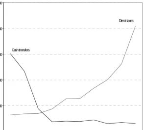
This conclusion is not fully warranted because our data take into account cash transfers only. Overall cash transfers in our database are in most cases (58 out of 68) less than taxes.21On average, direct taxes are 1.6 times greater than cash transfers (Table 8). For example, in the case of the Netherlands and the US shown in Figure 4, the tax-to-transfer ratio is respectively 1.8 and 2.5. If we were to add to cash transfers transfers-in-kind (health, education, public administration etc.) that also are financed out of taxes, overall transfers would increase, and it is quite likely that, under some reasonable apportioning of benefits from transfers-in-kind, the median voter may come out as net beneficiary. Our database does not allow us to test this hypothesis. We thus have to move to a weaker formulation of the median voter hypothesis, that is, to test Corollary 3.22
Table 8. Net tax as percentage of disposable income Average Standard
deviation
Minimum (country) Maximum (country)
Fifth decile 3.6 13.6 -43.1 (Poland 95) 33.2 (Netherlands 94)
Sixth decile 9.8 12.9 -32.9 (Poland 95) 36.2 (Netherlands 94)
Average 5.7 13.1 -36.5 (Poland 95) 28.2 (Israel 79)
Memo: Tax-transfer ratio
1.6 0.7 0.2 (Russia 92) 3.4 (UK 74)
Note: Deciles formed according to household per capita factor income.
21
Note that taxes include both mandatory employee contributions and direct taxes. 22
Table 4. Cash transfers and direct taxes by decile (deciles formed according to factor income)
United States 1997 The Netherlands
1994
Note: Amounts on the vertical axis in local currency. 0 5000 10000 15000 20000 1 2 3 4 5 6 7 8 9 10 Cashtransfers Direct taxes 0 5000 10000 15000 20000 25000 1 2 3 4 5 6 7 8 9 10 Cashtransfers Direct taxes
We test Corollary 3 by looking at the relationship between R, the share gain of the middle class (fifth and sixth decile according to factor income), andµthe position of the median voter (at the factor income level), and other variables Z, in:
(2) R= f(
µ
,Z)Similar to the sharegain definitions above, we define the share gain of the middle class as the change in the percentage of total income received by the fifth and sixth decile as we move from factor to disposable income (sharegain5060). µis alternatively defined as the factor income share of the middle class (Share5060MM), and median income expressed as percentage of mean income. In both formulations, we expect that an improvement in the relative position of the middle class in distribution of factor income will reduce its share gain. The regressions are for both definitions of factor income (factor income and factor P income).
The variable sharegain5060 is in all cases negative (see Annex Table 6). The mean
sharegain5060 is minus 6 percentage points, and the range is from –12.1 (Belgium 1985) to
–1.3 (Sweden 1995). The situation is the same if sharegain is defined with respect to factor P income. The mean sharegain5060 is then minus 4.5 percentage points and the range is from -14.5 to -1.1. But we expect that the sharegain will be greater in countries where the position of the middle class, before taxes and transfers “kick in”, is worse.
Table 9 gives the results. A percentage point decrease in the factor income share of the middle class is associated with a 0.4 point increase in middle class share gain. The coefficient is significant at the 1 percent level in both formulations. However, the R2’s are much lower than in the test of the redistribution hypothesis. The result that the coefficient is less than 1 implies that redistribution does not fully “compensate” the middle class in a more unequal country for its lower factor income share.
Regressions 2.1 and 2.2 (Table 9) test the same hypothesis using the mean-to-median ratio as a proxy for the position of the middle class at the factor income level. With factor income, we see that a 10 percent increase in the ratio—that is, a less favorable position of the middle class—raises the sharegain of the middle class by 1.3 percentage points.
When we use factor P income, the values of the coefficients are about the same but their level of significance decreases and R2becomes practically zero. This means that once we eliminate pensions from cash transfers, the middle classes’ gain or loss in redistribution is independent of the initial (factor) distribution. This is explained by the fact that middle
classes receive little in the form of non-pension cash transfers such as unemployment benefits, social assistance and even family allowances. Thus the median voter hypothesis fails when we focus on the truly redistributive transfers only.
Table 9. Middle class gain as function of initial position of the median voter ( fixed effect regresions)
Using factor income Using factor P income All sample Established
democracies
All sample Established democracies Independent variables (1) Sharegain5060 (2) Sharegain5060 (3) Sharegain5060 (4) Sharegain5060
(1) Middle class share (share5060MM) -0.443 (-5.08) -0.417 (-3.76) -0.389 (-2.81) -0.444 (-2.86) Age over 65 (%) 0.081 (0.59) 0.094 (0.67) Constant 11.14 (2.51) 9.78 (1.83) 11.67 (2.02) 14.09 (2.16) R2 (F) 0.09 (15.4) 0.13 (8.3) 0.16 (7.9) 0.01 (7.9) (2) Mean-to-median ratio 12.94 (4.66) 13.01 (3.59) 12.04 (2.56) 13.33 (2.52) Age over 65 (%) 0.093 (0.66) 0.101 (0.7) Constant -23.05 (-6.88) -23.32 (-5.3) -19.09 (-3.36) -20.44 (-3.19) R2 (F) 0.08 (13.4) 0.13 (7.7) 0.01 (6.6) 0.01 (6.4) Number of observations 79 67 79 67
Note: t-values between brackets. Share5060MM=share of total factor income received by the fifth and sixth decile of the population ranked by factor income (=middle class). haregain5060=middle class gain as one moves from factor to disposable income. All R2’s are overall.
5. Conclusions
The purpose of this study has been twofold: (1) to test the hypothesis of an inverse relationship between inequality in distribution of factor income and redistribution, and (2) to test one possible explanation for redistribution, the political collective-choice mechanism through the median-voter hypothesis.
The approach taken in the paper is novel, in that, for the first time, both the median-voter hypothesis and the dependent and the independent variables in the redistribution equations are correctly specified. The dependent variable is the extent of redistribution—the income share gain of the lower half of income distribution according to factor income (‘the poor”), or of the bottom quintile (”the very poor”), or the middle class (fifth and sixth decile). The independent variable is inequality of factor incomes or the position of the middle class in factor income distribution. Neither of these two variables was used in previous research, because they have not been readily available. The data has been for a sample of 24 countries, with a total of 79 observations.
The results show strong support for the redistribution hypothesis. More unequal factor-income countries redistribute more toward the poor and very poor. A country A with exactly the mean characteristics of the sample would have a factor Gini coefficient of 46.3, and the bottom half of its population (“the poor”) would receive 19.4 percent of total factor income. When we move to disposable income distribution, that is, include all government cash transfers and personal taxes, the same average country would have a Gini of 32.2, and the same people will have increased their share to 32.1 percent of total disposable income. The poor will have therefore gained a 12.7 percentage point share.
Consider another country B, more unequal in terms of its factor income distribution. Let the poor’s factor income share be 1 point less than their share share in country A. Now, the redistribution in a more unequal country would be greater and the sharegain for the poor in country B would reach 13.7 percentage points, exactly 1 point more than in country A. The poor in both countries would therefore end up with the same share of disposable income. For the very poor (the bottom quintile), redistribution is even stronger making their position in terms of disposable income share negatively related to their starting position (factor-income share).
The effects of redistribution become more muted when pensions are taken out of transfers and treated as factor income. The negative sign between the poor’s share in factor
income and share gain persists, and the coefficient remains statistically highly significant throughout, but is much smaller. Now, redistribution compensates for only 70 percent of the poor’s initial shortfall in a more unequal country (i.e. the poor in country B will no longer be able to “catch up”, in terms of disposable income, with the poor in country A), and for a little lover 90 percent of the very poor’s shortfall.
While the evidence supports the link between the extent of pro-poor redistribution and factor income inequality, the evidence that redistribution takes place through the median voter channel is much weaker. The data—based on cash transfers only—do not allow us to conclude that the middle class is a net beneficiary of redistribution. Comparing cash transfers and taxes only, the middle-income groups appear invariably to be losers.
However, it is likely that, if we included transfers in kind, the middle classes may turn out to be net beneficiaries. When we test a weaker formulation of the median voter hypothesis—namely that lower factor income shares of the middle class are associated with a greater share gain—we find that the relation holds when pensions are included among cash transfers. When pensions are excluded, there is much less evidence that the middle classes starting from a less favorable factor income position redistribute more in their own favor.
The median voter hypothesis thus fails when we focus on the truly redistributive transfers. The middle classes contemporaneously gain little from these transfers. This leaves us looking for explanations.
First, since those poorer than the middle classes contemporaneously gain, perhaps the decisive voter is at a level income lower than the median? This seems implausible. Recent research has, if anything, moved in the direction of the conclusion that the decisive voter at a level higher than the median (see Bassett, Burkett and Putterman, 1999).
Second, the absence of contemporaneous middle-class gain may mask a long-run middle-class gain from redistributive programs. Those currently in the middle class may not profit from current social transfers. They may however be willing to finance the transfers as insurance for themselves (they for example receive transfers if they become unemployed).
Third, and most problematically for previous studies, the median-voter hypothesis may not be the appropriate collective-decision making mechanism to explain redistribution decisions. The median-voter hypothesis is based on direct voting. Other than in Switzerland (an in various degrees amongst cantons; see Feld and Kirchgässner 2000), collective
Since direct voting does not take place on every issue, the median-voter hypothesis applied to voters does not describe the collective decision-making rule. Under representative
democracy, the median-voter hypothesis could apply for an issue on which an election outcome is decided. There is therefore a question whether, and to which extent, policy outcomes for an issue under representative democracy reflect the preferences of the median voter. The results that are reported in this paper suggest broad-ranging outcomes where the institutions of representative democracy do not result in the redistribution that would be sought by the median voter.
Acknowledgements
I thank Costas Krouskas and Yvonne Ying for research assistance. Roberta Gatti , Mark Gradstein, Arye L. Hillman, Phil Keefer, Mattias Lundberg, Louis Putterman, Tine Stanovnik, Heinrich Ursprung, two anonymous referees, as well as to the participants in the 1999 Silvaplana Workshop on Political Economy, and World Bank Inequality Thematic Group where the paper was presented, provided useful comments. The research was financed in part by a World Bank Research Grant RPO 683-01.
REFERENCES
Alesina, A., Rodrik, D., 1994. Distributive politics and economic growth. Quarterly Journal of Economics 109, 465-90.
Alesina, A., Perotti, R., 1994. The political economy of growth: A critical survey of the recent literature. The World Bank Economic Review 8, 350-371.
Bassett, W. F., Burkett, J.P., Putterman, L., 1999. Income distribution, government transfers, and the problem of unequal influence. European Journal of Political Economy 15, 207-228. Bertola, G., 1993. Factor shares and savings in endogenous growth. American Economic Review 83, 1184-1198.
Easterly, W., Rebelo, S., 1993. Fiscal policy and economic growth: an empirical investigation. Journal of Monetary Economics 32, 417-458.
Esping-Andersen, G., 1990. The Three Worlds Of Welfare Capitalism. Princeton University Press, Princeton, N.J.
Feld. L.P., Kirchgässner, G., 2000. Direct democracy, political culture and the outcome of economic policy: A report on the Swiss experience. European Journal of Political Economy 16.
Le Grand, J., 1982. The Strategy of Equality: Redistribution and the Social Services. Allen and Unwin, London.
Milanovic, B., 1999. World income distribution in 1988 and 1993. The World Bank, Washington, D.C.
Perotti, R., 1992. Income distribution, politics and growth. American Economic Review 82, 311-316.
Perotti, R., 1993. Political equilibrium, income distribution, and growth. Review of Economic Studies 60, 755-76.
Perotti, R., 1996. Growth, income distribution, and democracy: What the data say. Journal of Economic Growth 1, 149-187.
Persson, T., Tabellini, G., 1991. Is inequality harmful for growth?: Theory and evidence. National Bureau of Economic Research, working paper no. 3599.
Persson, T., Tabellini, G., 1994. Is inequality harmful for growth?: Theory and evidence. American Economic Review 84, 600-621.
Persson, T., Tabellini, G., 1992. Growth, distribution and politics. European Economic Review 36, 593-602.
Annex Table 1. Gini coefficients
Factor income
Factor P income
Gross income Disposable income (4)-(1) Australia 81 46.0 41.9 37.7 33.4 -12.6 85 47.7 43.4 39.3 34.3 -13.4 89 48.5 45.1 39.7 35.0 -13.5 94 51.6 48.1 41.0 36.6 -15.1 Belgium 85 54.6 34.0 26.7 26.7 -27.8 88 50.0 34.4 26.9 26.9 -23.1 92 50.4 38.0 31.8 26.0 -24.4 Canada 75 43.8 40.8 37.2 34.8 -9.0 81 42.9 39.8 36.5 33.9 -9.1 87 44.2 40.4 36.6 33.3 -10.8 91 45.5 41.5 36.4 32.6 -12.9 94 47.0 42.2 36.9 32.9 -14.1 Czech Republic 92 43.7 30.0 24.0 21.7 -22.0 Denmark 87 44.3 38.0 30.7 27.8 -16.5 92 47.2 40.3 30.5 26.0 -21.2 Finland 87 36.4 32.5 28.5 23.3 -13.1 91 36.6 33.5 28.5 23.9 -12.7 95 42.1 39.2 30.2 25.5 -16.6 France 79 50.9 42.8 38.1 34.6 -16.3 81 40.5 39.3 32.7 -7.8
84 52.2 42.8 37.9 34.4 -17.8 France (b) 89 52.8 42.1 35.9 34.2 -18.6 W. Germany 73 40.3 40.2 32.5 31.1 -9.3 78 43.2 33.9 32.1 29.8 -13.4 81 44.1 34.8 31.4 29.4 -14.7 83 42.7 34.2 31.7 29.5 -13.2 84 47.9 35.5 33.1 29.3 -18.6 89 47.2 35.7 33.8 29.1 -18.0 94 50.4 39.4 35.9 31.2 -19.3 Hungary 91 52.0 39.2 30.3 30.3 -21.7 Ireland 87 55.6 53.2 41.7 37.7 -17.9 Israel 79 47.5 45.0 41.9 37.7 -9.9 86 50.7 47.7 43.2 37.8 -12.9 92 49.4 46.8 41.4 36.8 -12.6 Italy 86 46.1 34.0 33.7 -12.4 91 44.9 33.7 32.4 32.4 -12.5 95 51.3 39.8 37.6 37.6 -13.7 Luxembourg 85 41.7 32.6 27.9 -13.8 91 41.9 32.2 28.3 28.3 -13.6 94 44.0 33.1 28.0 28.0 -16.0 Netherlands 83 50.5 44.7 36.8 34.0 -16.6 87 49.7 44.3 35.6 32.7 -17.0 91 46.9 41.4 34.1 32.9 -13.9 94 45.0 40.0 34.0 33.8 -11.2
Norway 79 43.2 43.2 32.6 28.5 -14.7 86 39.5 39.5 29.0 25.5 -14.0 91 41.6 34.4 30.0 26.1 -15.5 95 44.3 36.5 30.5 26.7 -17.5 Poland 86 39.9 33.5 29.1 -10.8 92 45.9 36.3 33.8 33.8 -12.1 95 60.6 50.9 38.7 38.8 -21.7 ROC Taiwan 81 31.6 31.6 31.5 31.1 -0.5 86 31.4 31.4 31.3 30.8 -0.6 91 31.9 31.8 31.6 31.0 -0.9 95 32.9 32.1 31.4 31.0 -2.0 Russia 92 56.0 47.2 45.4 45.2 -10.8 95 62.0 50.0 48.8 48.8 -13.2 Slovak Republic 92 43.0 32.0 23.0 20.9 -22.1 Spain 80 45.9 45.9 35.7 35.7 -10.2 90 46.0 37.4 33.7 33.7 -12.4 Sweden 67 47.9 42.5 40.3 35.4 -12.4 75 45.6 35.6 31.1 25.5 -20.1 81 46.3 33.7 28.2 24.2 -22.0 87 47.5 34.1 29.2 25.5 -22.0 92 51.3 38.2 29.5 26.4 -24.9 95 50.4 40.5 29.9 26.2 -24.2 Switzerland 82 44.8 40.1 39.2 37.7 -7.1 U.K. 69 43.8 40.0 37.6 34.9 -8.9
74 39.3 34.9 33.8 31.1 -8.2 79 44.6 38.5 33.0 30.1 -14.5 86 52.6 46.6 37.5 34.3 -18.3 91 52.5 47.6 40.4 37.5 -15.0 95 54.7 50.0 41.2 38.1 -16.6 U.S.A. 74 46.8 42.7 41.1 37.8 -9.0 79 46.4 43.4 40.7 36.4 -9.9 86 48.7 45.0 43.1 39.2 -9.5 91 49.7 45.8 43.4 39.5 -10.2 94 52.4 48.3 45.9 41.7 -10.7 97 52.6 48.4 46.4 42.2 -10.3 Mean 46.4 39.8 35.0 32.2 -14.2 St. Deviation 5.9 5.6 5.5 5.3 5.5
Annex Table 2
GAIN IN SHARES (in percent;
using factor income)
Countries, years first Second Third Fourth fifth Five deciles (cumul) Australia 81 4.5 3.1 1.0 0.4 0.1 9.0 85 4.2 3.3 1.2 0.6 0.2 9.4 89 4.2 3.5 1.3 0.5 0.2 9.6 94 4.0 4.2 2.0 0.7 0.2 11.1 Belgium 85 8.8 9.0 8.7 1.5 -0.8 27.3 88 8.6 8.5 3.7 2.3 -0.3 22.9 92 8.9 4.8 4.4 1.2 0.1 19.5 Canada 75 3.3 1.7 1.0 0.5 0.2 6.7 81 3.5 1.7 1.0 0.5 0.2 6.8 87 4.1 2.2 1.3 0.7 0.2 8.4 91 4.4 2.7 1.7 0.9 0.3 10.0 94 4.8 3.0 1.9 1.0 0.4 11.1 Czech Republic 92 9.2 5.4 2.0 0.7 -0.2 17.2 Denmark 87 8.0 5.7 2.9 0.8 -0.4 17.1 92 6.6 6.0 3.3 1.5 0.1 17.5 Finland 87 4.4 2.6 1.6 0.9 0.4 9.9 91 4.1 2.5 1.6 1.0 0.4 9.6 95 5.1 3.4 2.2 1.5 0.8 12.9 France 79 8.5 4.1 1.5 0.8 0.3 15.2