ECG Classification with an Adaptive Neuro-Fuzzy Inference System

(1)

ECG CLASSIFICATION WITH AN ADAPTIVE NEURO-FUZZY INFERENCE SYSTEM

A Thesis presented to

the Faculty of California Polytechnic State University, San Luis Obispo

In Partial Fulfillment of the Requirements for the Degree

Bachelor of Science and

Master of Science in Electrical Engineering

by

Brad Thomas Funsten June 2015

(2)

(3)

COMMITTEE MEMBERSHIP

TITLE: ECG Classification with an Adaptive Neuro-Fuzzy Inference System

AUTHOR: Brad Thomas Funsten

DATE SUBMITTED: June 2015

COMMITTEE CHAIR: Xiao-Hua (Helen) Yu, Ph.D. Professor of Electrical Engineering

COMMITTEE MEMBER: Jane Zhang, Ph.D.

Professor of Electrical Engineering

COMMITTEE MEMBER: John Saghri, Ph.D.

(4)

ACKNOWLEDGMENTS

I would like to thank my friends and family for their enormous support in completing this thesis. I would like to thank Dr. Yu for her advice and counseling in accomplishing a project such as this. To all the engineers at Advanced Telesensors, Inc., thank you so much for your insight that paved the way for the thesis. I want to thank my doctor, Dr. Gazarian, for giving me a free ECG test.

I want to emphasize that completing this thesis would not be possible without the support of friends and family. Whether it was school, church, or home, the power of encouragement and fun times allowed me to persevere. Proofreading from family and friends was much appreciated. Thank you all!

(5)

ABSTRACT

ECG Classification with an Adaptive Neuro-Fuzzy Inference System Brad Thomas Funsten

Heart signals allow for a comprehensive analysis of the heart. Electrocardiography (ECG or EKG) uses electrodes to measure the electrical activity of the heart. Extracting ECG signals is a non-invasive process that opens the door to new possibilities for the application of advanced signal processing and data analysis techniques in the diagnosis of heart diseases. With the help of today’s large database of ECG signals, a computationally intelligent system can learn and take the place of a cardiologist. Detection of various abnormalities in the patient’s heart to identify various heart diseases can be made through an Adaptive Neuro-Fuzzy Inference System (ANFIS) preprocessed by subtractive clustering. Six types of heartbeats are classified: normal sinus rhythm, premature ventricular contraction (PVC), atrial premature contraction (APC), left bundle branch block (LBBB), right bundle branch block (RBBB), and paced beats. The goal is to detect important characteristics of an ECG signal to determine if the patient’s heartbeat is normal or irregular. The results from three trials indicate an average accuracy of 98.10%, average sensitivity of 94.99%, and average specificity of 98.87%. These results are comparable to two artificial neural network (ANN) algorithms: gradient descent and Levenberg Marquardt, as well as the ANFIS preprocessed by grid partitioning.

Keywords: ECG, Fuzzy Logic, Adaptive Neuro Fuzzy Inference System, ANFIS, Computational Intelligence, Neural Network, ANN, Signal Processing

(6)

TABLE OF CONTENTS Page LIST OF TABLES ... ix LIST OF FIGURES ... xi CHAPTER 1: INTRODUCTION ... 1 1.1: Project Goal ... 1 1.2: Overview ... 1 1.3: Software Environment ... 1 1.4: Research Importance ... 2 1.5: Past Research ... 4 1.6: Brief Approach ... 4 2: BACKGROUND ... 6 2.1: Electrocardiography ... 6 2.2: Human Heart ... 9 2.3: Heart Abnormalities ... 11

2.4: Fuzzy Set Theory ... 16

2.5: ANFIS Algorithm ... 20

2.6: Hybrid Learning Algorithm ... 25

2.7: ANFIS Overview ... 31

2.8: Subtractive Clustering as a Preprocessor to ANFIS Classification ... 32

3: LITERATURE REVIEW ... 37

3.1: Time Domain Based Classifier for ECG Signals ... 37

3.2: Radial-Basis-Function (RBF) Neural Network with the Genetic Algorithm for ECG Classification ... 38

(7)

3.4: Adaptive Parameter Estimation Using Sequential Bayesian Methods for

ECG Classification ... 42

3.5: Fast Fourier Transform and Levenberg-Marquardt Classifier for ECG Signals ... 44

3.6: Support Vector Machine (SVM) and Wavelet Decomposition for ECG Classification ... 46

3.7: Past Research on ANFIS for ECG Classification ... 47

4: CLASSIFICATION APPROACH ... 50

4.1: ANFIS of ECG Signals ... 50

4.2: Extracting Input Features ... 55

4.3: Program Flow ... 63

4.4: Performance Evaluation Method ... 67

5: SIMULATION RESULTS ... 68

5.1: ANFIS on Several ECG Records under Subtractive Clustering ... 68

5.2: Justification of Chosen Input Records ... 85

5.3: Comparison to ANN ... 86

5.4: Comparison to ANFIS under Grid Partitioning ... 96

6: CONCLUSIONS AND FUTURE WORKS ... 104

REFERENCES ... 106

APPENDICES ... 109

APPENDIX A – List of Acronyms ... 109

APPENDIX B – MATLAB Code ... 110

Plot ECG Signal from MIT-BIH Arrhythmia Database with Annotations: ... 110

ECG Input Layer: ... 114

Input to ANFIS for One ECG Signal: ... 139

Input to ANFIS for Multiple ECG Signals: ... 140

ANFIS (grid partitioning or subtractive clustering) for ECG Signals and Evaluation of Test Data: ... 150

(8)

Comparison with ANN (Gradient Descent and Levenberg-Marquardt: ... 155 APPENDIX C – Project Analysis ... 157

(9)

LIST OF TABLES

Table Page

1: Hybrid learning applied to ANFIS [15] ... 25

2: Input features of an ECG signal [5], [8], [24] ... 52

3: MIT-BIH records and corresponding heartbeat types: ‘N’ being normal, ‘V’ being PVC, ‘A’ being APC, ‘L’ being LBBB, ‘R’ being RBBB, and ‘P’ being paced beats ... 58

4: The seven features associated with a corresponding input number ... 68

5: Heartbeats (including each heartbeat type) chosen from records of the MIT-BIH database randomly ... 69

6: Trial 1 training and checking results for the six ANFIS’ ... 78

7: Trial 1 classification results for the six ANFIS’ ... 79

8: Analysis of a PVC and LBBB heartbeat that were classified incorrectly ... 80

13: Average accuracy, sensitivity, and specificity results for 3 trials for subtractive clustering preprocessed ANFIS ... 85

14: Trial training and checking results for the six ANFIS training and checking data for gradient descent ... 88

15: Trial 1 classification results for the six gradient descent neural networks (NN) ... 89

16: Trial 2 training and checking results for the six ANFIS training and checking data for gradient descent ... 89

(10)

18: Trial 3 training and checking results for the six ANFIS training and checking data for

gradient descent ... 90

19: Trial 3 classification results for the six gradient descent neural networks (NN) ... 91

20: Average accuracy, sensitivity, and specificity results for 3 trials for gradient descent ... 91

21: Trial 1 training and checking results for the six ANFIS training and checking data for Levenberg-Marquardt ... 93

22: Trial 1 classification results for the six Levenberg-Marquardt neural networks (NN) ... 93

27: Average accuracy, sensitivity, and specificity results for 3 trials for Levenberg-Marquardt ... 95

28: Trial 1 training and checking results for the six grid partitioned ANFIS’ ... 99

29: Trial 1 classification results for the six gradient partitioned ANFIS’ ... 100

31: Trial 2 classification results for the six grid partitioned ANFIS’... 101

33: Trial 3 classification results for the six grid partitioned ANFIS’... 102

34: Average accuracy, sensitivity, and specificity results for 3 trials for grid partitioned ANFIS ... 102

35: Different membership function type average accuracy, sensitivity, and specificity results For 3 trials for grid partitioned ANFIS ... 103

(11)

LIST OF FIGURES

Figure Page

1: ECG signal showing two PVCs detected and corresponding degree of fulfilment versus

ANFIS decision rule [7] ... 3

2: ECG signal [23] ... 6

3: ECG device ... 7

4: ECG Paper ... 7

5: Ten electrodes (Twelve-leads) [9] ... 8

6: The human heart [27] ... 9

7: Illustrative ECG relation to the human heart [27] ... 10

8: Example of a PVC beat from MIT-BIH database, record 100, lead: Modified Limb Lead II (MLII) ... 11

9: Example of an APC beat from MIT-BIH database, record 100, lead: Modified Limb Lead II (MLII) ... 12

10: Example of a LBBB from MIT-BIH database, record 109, lead: Modified Limb Lead II (MLII) ... 13

11: Example of a RBBB from MIT-BIH database, record 118, lead: Modified Limb Lead II (MLII) ... 14

12: Example of a paced beat from MIT-BIH database, record 104, lead: Modified Limb Lead II (MLII) ... 15

13: Several membership functions µ to choose from for a fuzzy set Z ... 17

14: FIS diagram [12] ... 18

15: n-input first-order Sugeno Adaptive Neuro-Fuzzy Inference System (ANFIS) [12] ... 23

16: Two-input, two-rule, first order Sugeno ANFIS model [12] ... 24

(12)

18: Process of classification ... 50

19: Several temporal input features of an ECG signal [6] ... 51

20: RR previous interval (RRp) and RR subsequent interval (RRs) input features [6] ... 51

21: Amplitude input features [6] ... 52

22: General ECG block diagram for this thesis ... 53

23: Method of classification with ANFIS ... 54

24: General ANFIS structure ... 55

25: The Pan-Tompkins algorithm for QRS complexes [21] ... 61

26: One heartbeat showing the results of the WFDB toolbox function ... 62

27: Histogram of normal P amplitudes ... 63

28: Classification program flowchart ... 66

29: RMSE training and checking curves for the first ANFIS under three membership functions for each input for 1000 iterations. Initial step size is 0.01 ... 70

30: RMSE training and checking curves for the first ANFIS under three membership functions for each input for 1000 iterations. Initial step size is 0.001. Convergence was reached at 78 iterations ... 71

31: Step curve for the first ANFIS under three membership functions for each input for 1000 iterations. Initial step size is0.001 ... 72

32: Initial subtractive clustering FIS for the first ANFIS. The solid dark function represents the first membership function. The dashed function represents the second membership function. The gray function represents the third membership function ... 73

33: Adaptive FIS for the first ANFIS. The solid dark function represents the first membership function. The dashed function represents the second membership function. The gray function represents the third membership function ... 74

(13)

34: Antecedent and consequent parameters before and after training for subtractive clustering FIS. This is the first input's first membership function parameters for the antecendent parameters and the first rule's consequent parameters... 75 35: Decision surface generated from the first ANFIS after 246 iterations between the first

input (QRS interval) and the fifth input (RR ratio) ... 76 36: Trial 1 RMSE training and checking curves for the six ANFIS' (1-6) under three membership .... 77 37: Trial 2 RMSE training and checking curves for the six ANFIS' (1-6) under three membership functions for each input ... 81 38: Trial 3 RMSE training and checking curves for the six ANFIS' (1-6) under three membership functions for each input ... 83 39: Neural network structure for gradient descent and Levenberg-Marquardt algorithms ... 87 40: Trial 1 RMSE training and checking curves for the first ANFIS training and checking data for gradient descent. Convergence was reached at 566 iterations from overfitting

(minimum checking RMSE reached) ... 88 41: Trial 1 RMSE training and checking curves for the first ANFIS training and checking data for Levenberg-Marquardt. Convergence was reached at 13 iterations from overfitting

(minimum checking RMSE reached) ... 92 42: Trial 1 RMSE training and checking curves for the first ANFIS under two membership

functions grid partitioned for each input for 100 iterations. Initial step size is 0.01.

Convergence was reached ... 96 43: Trial 1 initial grid partition FIS for the first ANFIS. The solid dark function represents the first membership function. The dashed function represents the second membership function ... 97 44: Trial 1 adapted FIS for the first ANFIS. The solid dark function represents the first

membership function. The dashed function represents the second membership function ... 98 45: Antecedent and consequent parameters before and after training for grid partition FIS ... 99

(14)

CHAPTER 1: INTRODUCTION

1.1: Project Goal

Electrocardiograph (ECG) signal tests allow detection of various characteristics in a patient’s heart. Characteristics include abnormalities, size and position of chambers, damage to tissue, cardiac pathologies present, and heart rate. The problem with today’s ECG signal instruments is the inability to characterize the signals without a doctor’s complete evaluation and diagnosis [28]. Research in the field of Computational Intelligence gives promising research results in order to solve this problem. An Adaptive Neuro-Fuzzy Inference System (ANFIS) is a type of neuro-fuzzy classifier and is one of many areas of study in Computational Intelligence (CI). The goal of this project is to explore various

applications of an ANFIS to classify well known ECG heartbeats. An additional goal is to compare the ANFIS with artificial neural network (ANN) algorithms.

1.2: Overview

This thesis informs the reader in Chapters 1-4 of theoretical aspects and methodology behind ECG classification. Chapters 5 and 6 present results through simulation and experimentation as well as conclusions and future works. The MATLAB code and a project analysis report can be found in the appendices.

1.3: Software Environment

Simulations and programs for this thesis were programmed through MATLAB® 8.1.0.604 (R2013a) 32-bit version. This environment was selected because of its simplicity in programming and debugging signal processing and matrix-based mathematical operation programs. An extensive number of integrated functions for viewing and analyzing ECG signals as well as optimized matrix math operations greatly accelerated development through MATLAB. This project was made possible through

(15)

the MATLAB® NEURAL NETWORK TOOLBOXTM version 8.1.0.604 and MATLAB® FUZZY LOGIC TOOLBOXTM version 2.2.17 additions to the MATLAB student version.

1.4: Research Importance

Cardiac arrhythmias are one of the reasons for high mortality rate. The study of ECG pattern and heart rate variability in terms of computer-based analysis and classification of diseases can be very helpful in diagnostics [15]. This thesis falls under the field of CI. Applications range from adaptive learning to speech recognition. The field draws from biological concepts such as the brain and the physiological decisions of organisms. Breakthroughs in applying CI to medical diagnosis have shown to be successful in the past and are thus important to heart signal classification [29]. This type of data processing could be effectively applied to other biometrics such as electroencephalograms (EEGs) or electromyography (EMGs) to detect the existence of abnormalities in the brain or muscles respectively [2].

The purpose of this study is to aid the cardiologist in diagnosis through neuro fuzzy model classifiers. The rules of neuro fuzzy model classifiers allow for an increase in the interpretability and understandability of the diagnosis. A physician can easily check a fuzzy model classifier for plausibility, and can verify why a certain classification result was obtained for a certain heartbeat by checking the degree of fulfilment of the individual fuzzy rules [7].

1.5: Past Research

Classsifying heartbeats have been performed through an adaptive neuro-fuzzy inference system (ANFIS). An ANFIS utilizes both fuzzy logic and ANNs to approximate the way humans process information through tuning rule-based fuzzy systems [14]. An ANN is a neural network that is a semi-parametric, data-driven model capable of learning complex and highly non-linear mappings [1]. It is to be noted that both the ANFIS and ANN are supervised learning networks. This means a “teacher” must be present in the form of training data in order to train, validate, and test the network. An ANFIS approach to classification between a normal heartbeat and a premature ventricular contraction (PVC) heartbeat has

(16)

been studied with the ANFIS producing classification results at a faster convergence than the ANN in addition it allows for human interpretability. The only limitation is its computational complexity. A PVC is an abnormal heartbeat that is characterized as an extra heartbeat.

A decision, whether positive or negative, is exclusively from the ANFIS rule-based structure. Classification between normal and PVC heartbeats achieved an accuracy of 98.53%. [7]. Figure 1 shows the detected PVCs out of normal beats (N), and a graph showing the degree of fulfillment versus the particular rules needed to detect the PVCs. For a more complete analysis of past research in terms of different algorithms of classifying ECG signals, see Chapter 3.

Figure 1: ECG signal showing two PVCs detected and corresponding degree of fulfilment versus ANFIS decision rule [7]

(17)

1.6: Brief Approach

For ECG classification, a database of signals is used to observe and extract features. The MIT-BIH (Massachusetts Institute of Technology-Beth Israel Hospital) Arrhythmia Database consists of 48 half-hour excerpts of two-channel ambulatory ECG records which were obtained from 47 subjects studied by the BIH Arrhythmia Laboratory between 1975 and 1979. The sampling rate of the recordings is 360 samples per second. The bit resolution is 11 bits. The amplitude range is 10 mV. Two cardiologists have made the diagnosis for these various records and they have annotated each cardiac cycle. The annotations are important for learning in the neuro-fuzzy classifier [20].

Before classification, the database signals are preprocessed for both observation and training. Preprocessing includes passing the signal through a low-pass filter to remove the 60 Hz power noise for ease of observation of the signal. The given signal would have a baseline shift and would not represent the true amplitude therefore a high pass filter is then used to detrend the signal to direct current (DC) baseline level in order to obtain amplitude information from the signals [19]. The cardiologist’s

annotations of each heartbeat for each ECG signal are then read from a downloadable MATLAB package from the online database. A pre-made algorithm for detecting the various parts of an ECG signal is then applied to complete the annotation.

ANFIS would classify each heartbeat of an ECG signal. For example, the ANFIS is used here to classify between normal and abnormal heartbeats. It is a binary classifier and thus has one output to the network [15]. The normal and abnormal heartbeats are discussed in Section 2.3. The annotations of each ECG signal allow for inputs to the classifier to be trained. These inputs are different characteristics of an ECG signal. The characteristics are usually temporal intervals and amplitudes of the various parts of the signal. The inputs are then passed through an ANFIS for classification.

To summarize the limitations with traditional methods and advantages over conventional methods for the ANFIS, we begin with convergence speed. It has been shown that the ANFIS has a faster

convergence speed than a typical ANN. This is due to a smaller fan-out for backpropagation and the network’s first three layers are not fully connected. Smoothness is also guaranteed by interpolation.

(18)

Limitations are computational complexity restrictions. This is due to the exponential complexity of the number of rules for grid partitioning. There are surface oscillations around points caused by a high partition of fuzzy rules for grid partitioning. A large number of samples would slow down the subtractive clustering algorithm. Grid partitioning and subtractive clustering are discussed in Section 2.4. [15].

(19)

CHAPTER 2: BACKGROUND 2.1: Electrocardiography

Electrocardiography (ECG or EKG) is an approach to measuring the heart’s electrical activity. It is typically a non-invasive approach to detecting abnormalities in the heart. Figure 2 shows an ECG signal with various characteristics. A typical heartbeat or cycle begins with a P wave followed by a QRS

complex. The beat then ends with a T wave. Occasionally, a U wave appears after the T wave.

Figure 2: ECG signal [23]

An ECG test can be performed by a local doctor. An ECG measuring device is usually twelve leads. Figure 3 shows this device. ECG interprets the heart’s electrical activity through amplitude over time. Ten electrodes are used in a twelve-lead ECG device. Six electrodes are placed across the chest. The remaining four electrodes are placed on the limbs: left arm (LA), right arm (RA), left leg (LL), and right leg (RL).

(20)

Figure 3: ECG device

The output of the ECG device is made up of signals from each of the twelve leads printed on a piece of paper. Figure 4 shows an example ECG signal printed on paper. From the paper, the doctor can diagnose the patient. The paper shows limb leads: I, II, III, and augmented leads: aVR, aVL, aVF, and the six chest leads: V1-V6. The three limb electrodes form both the limb leads and augmented leads. Figure 5 shows the placement of the twelve leads

(21)

Figure 5: Ten electrodes (Twelve-leads) [9]

Electrocardiography was developed by Willem Einthoven in 1901. He built a string galvanometer to detect low current in order to record the heart’s electrical activity. Instead of having an electrical system to perform electrocardiography, he used salt solutions to record results. Over the course of twenty years, the setup went from 600 pounds to 30 pounds. Computers and microelectronics increased the effectiveness of ECG treatment in terms of accuracy and reliability [20].

RA

LA

LL RL

(22)

2.2: The Human Heart

The heart is a muscular organ that pumps blood carrying oxygen and nutrients throughout the body through the circulatory system. Figure 6 shows the human heart. It is divided into four chambers: upper left and right atria; and lower left and right ventricles.

Figure 6: The human heart [27]

Figure 7 shows the human heart in terms of its electrical activity. In a normal ECG heartbeat there are five prominent points. The first is the P wave and corresponds to an atrial depolarization. This

happens after the sinoatrial (SA) node generates an impulse. The node is located in the right atrium. The second is the QRS complex and corresponds to atrial repolarization and ventricular depolarization. By this time the ventricular excitation is complete. There is then a ventricular repolarization through the T wave.

(23)

The depolarization repolarization phenomena of the heart muscle cells are caused by the

movement of ions. This is the essence of the heart electric activity. Movement of ions in the heart muscle cells is the electric current, which generates the electromagnetic field around the heart [8].

(24)

2.3: Heart Abnormalities

This section introduces five heart abnormalities. These beats are not life threatening but pose an abnormal characteristic that gives way to a disease.

Premature Ventricular Contraction (PVC):

A PVC is an extra heartbeat resulting from abnormal electrical activation originating in the ventricles before a normal heartbeat would occur. This means the purkinje fibers are fired at the ventricles rather than the sinoatrial node. PVCs are usually nonthreatening and are common among older people and patients with sleep disordered breathing. Frequent PVCs are due to physical or emotional stress, intake of caffeine or alcohol, and disorders that cause the ventricles to enlarge such as heart failure and heart valve disorders. Figure 8 shows an example PVC heartbeat.

Figure 8: Example of a PVC beat from MIT-BIH database, record 100, lead: Modified Limb Lead II (MLII)

(25)

PVCs have the following features [5]:

 Broad QRS complex with duration greater than 120 milliseconds.

 Single-repeated abnormal QRS morphology or multiple abnormal QRS morphology.  Premature with a compensatory pause (lengthened RR with subsequent heartbeat).  Either ST depression or T wave inversion in leads with dominant R wave or ST

elevation with upright T waves in leads with a dominant S wave.

Atrial Premature Contraction (APC):

An APC is an extra heartbeat resulting from abnormal electrical activation originating in the atria before a normal heartbeat would occur. This means the purkinje fibers are fired at the atria rather than the sinoatrial node. APCs are usually nonthreatening and are common among heathy young and elderly people. It can be perceived as a skipped heartbeat. Frequent APCs are mainly due to physical or emotional stress and intake of caffeine or alcohol. Figure 9 shows an example APC beat.

Figure 9: Example of an APC beat from MIT-BIH database, record 100, lead: Modified Limb Lead II (MLII)

(26)

APCs have the following features [5]:

 Narrow QRS complex with duration less than 120 milliseconds.  Shortened RR interval with previous heartbeat.

 Premature with a compensatory pause (lengthened RR interval with subsequent heartbeat).

Left Bundle Branch Block (LBBB):

A LBBB is a condition where the left ventricle contracts later than the right ventricle due to delayed activation of the left ventricle. Frequent LBBBs are mainly due to hypertension, inadequate blood supply to the heart muscles, and heart valve diseases. Figure 10 shows an example LBBB heartbeat.

Figure 10: Example of a LBBB from MIT-BIH database, record 109, lead: Modified Limb Lead II (MLII)

(27)

LBBBs have the following features [5]:

 Broad QRS complex with duration greater than 120 milliseconds.  ST wave is deflected opposite of the QRS complex.

 ST segments and T waves always go in the opposite direction to the main vector of the QRS complex.

Right Bundle Branch Block (RBBB):

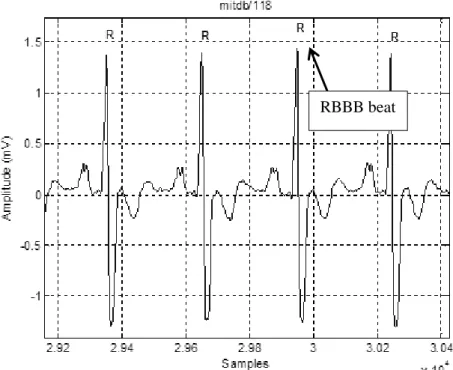
A RBBB is a condition where the right ventricle does not completely contract in the right bundle branch. The left ventricle contracts normally in the left bundle branch. Frequent RBBBs are mainly due to enlargement of the tissue in the right ventricles, inadequate blood supply to the heart muscles, and heart valve diseases. Figure 11 shows an example RBBB beat.

Figure 11: Example of a RBBB from MIT-BIH database, record 118, lead: Modified Limb Lead II (MLII)

(28)

RBBBs have the following features [5]:

 Broad QRS complex with duration greater than 120 milliseconds.  Slurred S waves.

 T waves deflected opposite the terminal deflection of the QRS complex.  ST depression and T wave inversion in the right precordial leads (V1-3)

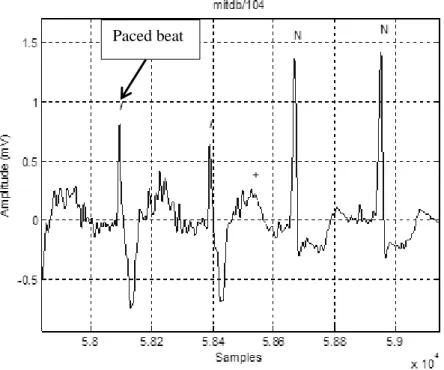
Paced beat:

A paced beat is the result of a patient with an artificial pacemaker. Figure 12 shows an example of a paced heartbeat.

Figure 12: Example of a paced beat from MIT-BIH database, record 104, lead: Modified Limb Lead II (MLII)

(29)

A paced heartbeat has the following features [7]:

 Vertical spikes of short duration (usually 2 milliseconds) before either the P or Q waves.

 Morphology on P or Q waves.

 Prolonged PR interval (280 milliseconds).

 Morphology on QRS complex. QRS complex resembles a ventricular heartbeatbeat.

2.4: Fuzzy Set Theory

Fuzzy sets provide a framework for incorporating human knowledge in the solution of problems. It is the basis of the ANFIS. In Fuzzy Logic theory, sets are associated with set membership. Compared to the traditional binary sets or “crisp sets” where membership is either ‘1’ typically indicating true or ‘0’ indicating false, fuzzy logic variables ranges between 0 and 1. Thus, Fuzzy Logic deals with approximate reasoning rather than fixed and exact reasoning [12].

The theory can be defined as follows. Let Z be a set of elements that is equivalent to z: Z {z}

Let A be a fuzzy set in Z characterized by a membership function,



_A

(

z

)

be a membership function that associates with each element of Z a real number in the interval [0, 1]. The elements, z, can be considered full, partial, or no membership to their corresponding membership functions. This can be expressed as

}

|

)

(

,

{

z

Z

A





_A



. Set theory can be applied to fuzzy sets. There is the possibility of empty sets, equivalent sets, complements, subsets, unions, or intersections. Common membership functions are gaussian, gaussian-bell, triangle, and trapezoidal shown in Figure 13 [12].

(30)

µ(z) z 1 µ(z) z 1 Triangle Trapezoidal µ(z) z Gaussian Bell 1 µ(z) z Gaussian 1

Figure 13: Several membership functions µ to choose from for a fuzzy set Z

A Fuzzy Inference System (FIS) formulates the mapping from a given input to an output using fuzzy sets. Figure 14 shows a FIS block diagram. The system comprises of five steps:

1. Fuzzification of the input variables

2. Application of the fuzzy operator (AND or OR) in the antecedent 3. Implication from the antecedent to the consequent

4. Aggregation of the consequents across the rules 5. Defuzzification

In Fuzzification, the inputs are mapped by membership functions to determine the degree to which the inputs belong.

In applying a fuzzy operator, the result of the antecedent and consequent of an if-then rule is found. From an antecedent or consequent, the fuzzy membership values can be found. An AND operator would take the minimum of the two limits of the fuzzy membership values. An OR operator would take the maximum of the two limits of the fuzzy membership values.

Implication from the antecedent to the consequent involves assigning weights to each rule. The consequent is a fuzzy set represented by a membership function, which weights appropriately the linguistic characteristics that are attributed to it. The consequent is reshaped using a function that either

(31)

truncates or scales the output fuzzy set. The input of the implication process is a single number given by the antecedent. The output is a fuzzy set. Implication is then implemented for each rule.

Next, aggregating all outputs of each rule into a single fuzzy set is done. Note this step should be commutative so that the order in which the rules are executed is unimportant. Three methods of

aggregations can be applied: maximum, probabilistic OR, or simply the sum of each rule’s output set. Defuzzification generates a single number from the aggregation step. The most popular method is the centroid calculation, which returns the center of area under the aggregate output curve. Other methods are bisector and average of certain ranges of the aggregate output curve [26].

Rule 1

Rule 2

Rule r

4. Aggregator 5. Defuzzifier 2. Apply Fuzzy Operator:

AND (min), or OR (max)

3. Implication from antecedent to consequent Input Output 1. Fuzzification If x is A1 AND/OR y is B1 If x is A2 AND/OR y is B2 If x is Ar AND/OR y is Br X y then f1 then f2 then fr

Figure 14: FIS diagram [12]

There are several fuzzy models for FIS. Two prominent models are the Mamdami and Sugeno models. The FIS discussed previously adheres to a Mamdami model. The Sugeno model however, determines the output not as a membership function, but as a constant or linear term.

The Sugeno fuzzy model is described as follows. Let

x



[

x

₁

,

x

₂

,....,

x

_n

]

Tbe the input vector and i

o

denote the output (consequent). Let

R

_idenote the ith rule, and

A

_i₁

,...,

A

_inare fuzzy sets defined in the antecedent space by membership functions



_Aij

(

x

_j

)

defined for all real numbers between ‘0’ and ‘1’. Let

(32)

) 1 ( 1

,...,

in

i

p

represent the consequent parameters and

M

is the number of rules. The set of rules and the

rule consequents are linear functions defined as:

:

i

R

if

x

₁is

A

_i₁and …

x

_nis

A

_inthen i

o

=

p

_i₁

x

₁+ …,

p

_in

x

_n+

p

_i₍_n_₁₎, i1,...,M

Defuzzification in the model is defined by a hyperplane in the antecedent-consequent product space. Let



_idenote the degree of fulfillment of the ith rule:





n

j ij j

i ₁

A

(

x

)



, i1,...,M

The output

y

of the model is computed through the center of gravity of the final fuzzy set [7]:



   _M i i M i i io y 1 1



There are several partitioning methods for FIS input spaces to form the antecedents of fuzzy rules. The grid partition consists of dividing each input variable domain into a given number of intervals whose limits do not necessarily have any physical meaning and do not take into account a data density repartition function [12]. Another is Subtractive clustering. This is a fast, one-pass algorithm for estimating the number of clusters and the cluster centers in a set of data. A data point with the highest potential is selected as a cluster center. Data points in the vicinity of the cluster center are removed to determine the next data cluster and center location. The process iterates until it is within radii of a cluster center. Section 2.5 discusses the ANFIS algorithm assuming grid partition. Section 2.8 discusses how the subtractive clustering can be used in conjunction with the ANFIS as an improvement instead of the grid partition in terms of rule reduction and overall classification of heartbeats. Both grid partition and subtractive clustering are simulated. Grid partition results are discussed in Section 5.4. Subtractive clustering results are discussed in Section 5.1 [26].

(1)

(2)

(33)

2.5: ANFIS Algorithm

An ANFIS, as mentioned before, combines the FIS with neural networks to tune the rule-based fuzzy systems. Two common FIS structures can then be applied: Sugeno or Mamdani. The Sugeno method is chosen in this thesis because it is computationally efficient, works well with linear techniques, works well with optimization and adaptive techniques, and it is well suited to mathematical analysis. The advantage of Mamdani is that it’s intuitive and well suited to human input. The disadvantage of Mamdani is it’s computationally expensive because another set of parameters is added to increase human

interpretablity.

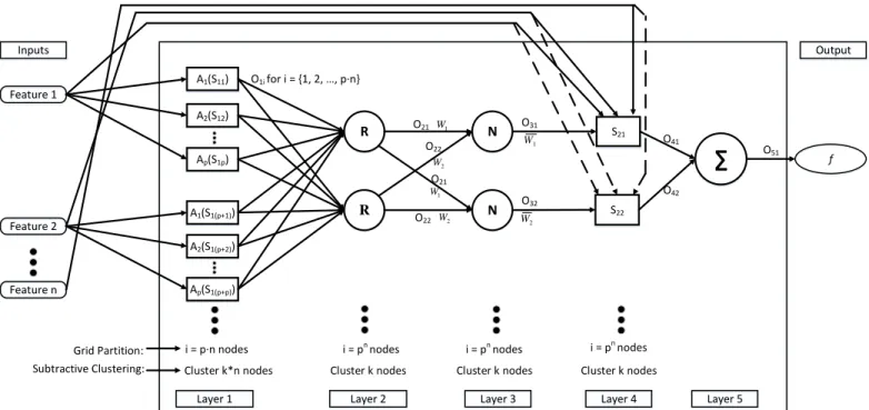
The Sugeno ANFIS has the premise part of the fuzzy rule as a fuzzy proposition and the conclusion part as a linear function. There are five layers of the structure discussed below and shown in Figure 15. A rectangle represents an adaptive node. Assuming a Sugeno fuzzy model, fuzzy-if-then rules are applied. This is shown in Figure 16. A first-order Sugeno ANFIS structure is used in order to output a linear function. A zero-order Sugeno ANFIS structure would output a constant parameter.

Parameters are calculated by the hybrid learning algorithm. Let S₁represent the antecedent (nonlinear) parameters and S₂represent the consequent (linear) parameters. The hybrid learning algorithm updates both parameters. This algorithm is discussed in Section 2.6.

Let n represent the number of inputs. Let

j

represent the layers of the ANFIS where

j

= {1, 2, 3, 4, 5}. Let output of node

i

of layers

j

beO_ji. Let

p

represent the number of membership

functions of each input.

Layer 1: This is the fuzzification layer. The output of this layer is

O

₁_iwherei{1,2,...pn}.

O

1iis a membership function that specifies the degree to which the given input satisfies the fuzzy sets

A

_k for

} ... , 2 , 1 { p

k . The fuzzy sets are represented as membership functions. The functions are expressed as

....})

,

{

;

(

x

t

a

b

c

d

Ak



for t{1,2,...n} where the input n features are grid partitioned into

p

membership functions. Each membership function is a function of the feature

x

_m.

(34)

....}) , , , , { ; ( 1i A xm ai bi ci di O 



_k

The membership functions represent the antecedent parameters of the ANFIS described as

...}

,

{

1i

a

i

b

i

c

i

S



. The new expression for the output

O

₁_iis as follows:

) ; ( 1 1i A xm Si O k





The nodes of this layer are adaptive. See Section 2.6 for details on adaptation of the antecedent parameters. There are several membership functions of fuzzy element z in the Sugeno structure that consist of antecedent parameters. They are listed as follows:

Gaussian: 2 ) ( 2 1 ) , ; ( b a z e b a z   



Where a represents the center and

b

represents the function’s width.

Gaussian-bell: c

b

a

z

c

b

a

z

2

|

1

1 )

,

;

(

_







Where a represents the center,

b

represents the function’s width, and crepresents both the direction of the bell and its width.

Triangle:



(z;a,b,c)

z

c

z

b

c

z

c

b

z

a

b

a

z

a

z











,

0 ,

,

0

Where

a



b



c

and{a,b,c}represents the z-coordinates of the three corners of the underlying triangle.

Trapezoid:



(z;a,b,c,d)

z

d

z

c

d

z

d

c

z

b

z

a

b

a

z

a

z











,

0 ,

,

1 ,

,

0 (6)

(7)

(8)

(9)

(4)

(5)

(35)

Where

a



b



c



d

and {a,b,c,d}represents the z-coordinates of the four corners of the underlying trapezoid.

Let

l

represent the number of antecedent parameters for each membership function



(z). The total number of antecedent parameters are then equivalent to:

Total number of antecedent parameters = l(pn)

Layer 2: This is the rule layer. The output of this layer is

O

₂_iwhere node

i



{

1 ,

2 ,

...

p

n

}

.

O

2iare rules that are defined either by an AND (minimum of incoming signals) or an OR (maximum of incoming signals).Let Rrepresent the rule choice of the second layer nodes in Figure 15.

]} {min[AND

R or R{max[OR]} Let

W

_irepresent the weights from the rule nodes.

}

{

2i

W

i

rule

A

k

O



Layer 3: This is the normalization layer. Let

N

represent the normalization of the nodes in layer 3 of

Figure 15. The output of this layer is

O

₃_iwhere node

i



{

1 ,

2 ,

...

p

n

}

. Let W_irepresent the normalized weight of each rule.

i i i i

W

O

...

2 1 3



_

Normalizing guarantees stable convergence of weights and biases. It also avoids the time-consuming process of defuzzification.

Layer 4: This is the defuzzification layer. The output of this layer is

O

₄_iwhere node

i



{

1 ,

2 ,

...

p

n

}

. Let

}

,

...

,

{

₁ ₂ 2i

q

i

q

i

q

np

r

i

S



n be the consequent parameters. A linear function

f

_iis expressed as the

multiplication of the inputs with the corresponding consequent parameters:

i n np i i i

q

x

q

x

q

x

r

f



₁ ₁



₂ ₂



...

n



The output

O

₄_iis the product of the normalized firing strength W_i with the linear function

f

_i:

(10)

(11)

(12)

(13)

(36)

) ... ( ₁ ₁ ₂ ₂ __ __ 4i Wi fi Wi qix q ix qnp xn ri O     n 

Total number of consequent parameters =

(

n



1 )



p

n

Layer 5: This is the summation layer. The output of this layer is

O

₅_iwhere nodei{1}. Since there is only one output, the ANFIS is a binary classifier. The output is the aggregation of all defuzzified outputs

i

O

₄ from layer 4, and thus it follows the center of gravity equation (3):



   i i i i i i i i i i W f W f W O O __ 4 51 for

{

1 ,

2 ,

...

}

n

p

i



x2 x1 Inputs Output A1(S11) A2(S12) A1(S1(p+1)) A2(S1(p+2)) R R N N S21 S22

∑

Layer 1 Layer 2 Layer 3 Layer 4 Layer 5

xn O1i for i = {1, 2, …, p·n} O21 O22 O22 O21 O31 O32 O41 O42 O51 i = pn _nodes i = p·n nodes i = pn _nodes _{i = p}n nodes Ap(S1p) Ap(S1(p+p)) f 1 W 2 W 1 W 1 W 2 W 2 W

Figure 15: n-input first-order Sugeno Adaptive Neuro-Fuzzy Inference System (ANFIS) [12]

(17)

(15)

(16)

(37)

An illustrated example of a two-input, two-rule, first order Sugeno ANFIS model is shown in Figure 16. µB1(x2) µA1(x1) µB2(x2) µA2(x1)

x

1

x

2 max min max min 2 1 2 2 1 1 51 W W f W f W O    2 2 1 1f W f W   1 W 2 W f1 = q11x1 + q12x2 + r1 f₂= q₁₂x₁+ q₂₂x₂+ r₂

(38)

2.6: Hybrid Learning Algorithm

Determination of optimal values of ANFIS parameters is made from a hybrid learning algorithm as discussed in [15]. It combines the least-squares estimator (LSE) method and the backpropagation gradient descent method for training. In the forward pass, the antecedent parameters are assumed fixed while the consequent parameters are identified by the LSE algorithm. In the backward pass, the consequent parameters are assumed fixed while the antecedent parameters are identified by the

backpropagation algorithm through gradient descent. This is described in Table 1. This algorithm could be made for both online and offline learning. However, this thesis uses the offline learning approach. As discussed in [37], the advantage of this algorithm is overall optimization of the consequent parameters for the given antecedent parameters. In this way we can, not only reduce the number of dimensions used in the gradient descent algorithm, but also accelerate the rate of convergence of the parameters.

Table 1: Hybrid learning applied to ANFIS [15] Forward pass Backward pass Antecedent parameters

(Non-linear) Fixed Gradient Descent Consequent parameters

(Linear) LSE Fixed

Signals Node outputs Error signals

Let S₁represent the set of the antecedent parameters and S₂represent the set of consequent parameters as discussed in Section 2.5. Following equation (17), we can develop an expression involving

the normalized weights Wi __

multiplied by the inputs

x

_t:

] ) ( ... ) ( ) [ __ __ 2 2 __ 1 1 __ 51



   i i i ni n i i i i ix q W x q W x q W r W O for

i



{

1 ,

2 ,

...

p

n

}

(18)

(39)

As discussed in [16], we can represent equation (18) as: ) ( ) ( ) ( 2 2 1 1f u X f u Xjfj u X y  

To identify the unknown consequent parameters

X

_l, usually a set of iterations (experiments) are

performed to obtain a training data set composed of data pairs

{(

u

_l

:

y

_l

),

l



1 ,



,

m

}

. Subsitiuting each data pair into equation (19) yields a set of mlinear equations:

m j m j m m j j j j

y

X

f

X

f

X

f

y

X

f

X

f

X

f

y

X

f

X

f

X

f













)

(

)

(

)

(

)

(

)

(

)

(

)

(

)

(

)

(

2 2 1 1 2 2 2 2 2 1 2 1 1 1 2 1 2 1 1 1

u







Let mand jrepresent the number of training data and consequent parameters respectively. Let

Arepresent a

m

x

j

matrix of weights multiplied by inputs as represented in equation (18). This can be represented as a design matrix denoted as:

           ) ( ) ( ) ( ) ( 1 1 1 1 m j m j f f f f u u u u A     

Let

X

represent a j x1vector of the unknown consequent parameters (assuming one rule

i



1

) be expressed as:















 1 1 1 11 1

r

X

q

X

q

X

j n j



X

and

y

represent a mx1output vector and equivalent as

O

₅₁for miterations:















m

y



1

y

(19)

(20)

(21)

(22)

(23)

(40)

Let the

l

th row of the joint data matrix



A



y



be denoted by



aT_l y_l



is related to the

l

th input-output data pair through:

)]

(

,

),

(

[

₁ _l _j _l T l

f

u

f

u

a





If Ais square (

m



j

) and nonsingular, then we can solve for

X

in the following equation: y AX To obtain:

y

A

X



1

However, usually this is an overdetermined solution (

m



j

) and thus the data might be

contaminated with noise. Thus an error vector eis used to account for this random noise and is expressed as:

y e AX 

A search for a minimum parameter (LSE) vector

X



X

*is made through a sum of squared error as discussed in [16]: ) ( ) ( ) ( ) ( 2 1 AX y AX y X a X 



     T m l T l l y E

The least squares estimator

X

*is found when the squared error is minimized satisfying the following equation:

y

A

AX

A

T *



T

If

A

T

A

is nonsingular and

X

*is unique, then the LSE is:

y

A

X

*



(

T

)

1 T

If

A

T

A

is singular, a sequential method of LSE is used. The sequential method of the LSE is the recursive least squares estimate and is used in this thesis. Here we assume the row dimensions of Aand

(24)

(25)

(26)

(27)

(28)

(29)

(30)

(41)

yarek, which represents a measure of time if the data pairs become available in sequential order. This means

X

_kis used to calculate

X

_k_₁:

Xk ATA ATy 1 ) (  































































 

y

T T T T T k

y

a

A

a

A

a

A

X

1 1

For simplification, we let

m

x

j

matrices

P

_kand

P

_k_₁be defined as: 1 ) (   A A Pk T 1 1 1

(

)

  

_











































T T T T T k

A

aa

a

A

a

A

P

The two matrices can be expressed as:

T k k P aa P  11 1 k

X

and

X

_k_₁can be expressed as:

)

(

1 1

y

T k k T k k

a

y

A

P

X

y

A

P

X





 

To express

X

_k_₁in terms of

X

_k, an elimination of

A

T

y

is made in equation (37):

k k T X P y A  1

Equation (37) is then plugged into equation (36) to obtain: ) ( 1 1 1 k k n y k P P X a X      1[( 11 ) k y] T k k P aa X a P       1 ( k) T k k P a y a X X    _

However, calculating

P

_k_₁involves an inversion calculation and is computationally expensive as explained in [16]. From equation (35), we have:

1 1 1 ( )     k  T k P aa P

(31)

(32)

(33)

(34)

(35)

(36)

(37)

(38)

(39)

(42)

A matrix inversion formula in [16] can be applied: 1 1 1 1 1 1

)

(

)

(

T



BC





T



T



B

I



CA



B



CT

 Let

T

and ICT1B

be nonsingular square matrices and letTP_k1,

B



a

, and CaT.

Then

P

_k_₁can be expressed as:

P_k 1 P_k P_ka(I aTP_ka) 1aTP_k     

a

P

a

P

aa

P

k T k T k k



_



1

In summary, the recursive LSE for equation (25) where the kth (1km)row of



A



y



denoted by



aT_k y_k



is sequentially obtained and is calculated as:

)

(

1

1 1 1 1 1 1 1 1 1 1 k T i k k k k k k k T k k T k k k k k

y

a

X

a

P

X

a

P

a

P

a

P

         













where kranges from 0 to m-1 and the overall LSE

X

*is equal to

X

_m(the consequent parameters

S

₂for all

i

rules in the ANFIS), the estimator using mdata pairs. In order to initialize the algorithm in equation (43), initial values of

X

₀and

P

₀is set. In practice [16] and in the thesis,

X

₀is set to a zero matrix for

convenience and

P

₀is expressd as:

I

P

₀





 is set to a positive large number to fulfill the following condition as explained in [16]:

0

1 lim

lim

___

P

₀1



___

I





 

The gradient descent backpropagation can be applied once the parameters in S₂are identified through equation (42). In the backward pass, the derivative of the error measure w.r.t each node output (including layer 5 of the ANFIS) toward the input end is determined, and thus the parameters of S₁are updated by the gradient descent backpropagation algorithm.

(40)

(41)

(42)

(43)

As was discussed in Section 2.5, let the output of node

i

of layers

j

beO_ij. In the ANFIS there are five layers: j{1,2,3,4,5}. The node outputs depend on both the incoming signals and its parameter set in S₁ {a,b,c,...}. Let

t

represent the number of nodes for the j1 layer. The node output can then be expressed as:

,...)

,

,...

(

O

₁ 1

O

1

a

b

c

O

_ij



_ij j _tj

Assume the given training data set has Pentries. Let E_prepresent an objective function that is a

function of an error measure for the

p

th (1 pP) entry of training data. This is equivalent to the difference of the target output vector

T

_Pand the actual output vector of layer 5, O5_p:

2 5

)

(

2

1

p p p

T

O

E





Let the error rate be represented as ₅ p p

O

E



and calculated as:

)

(

5 5 p p p p

O

T

O

E







Let zrepresent the number of nodes for the

j

th layer. An internal node error rate can be expressed through the chain rule:



  

_







z m j p i j p m j p m p j p i p

O

E

O

E

1 1 , , , 1 ,

Let represent an antecedent parameter of the ANFIS. LetO*represent all nodes that depend on  , then we have:











N O p

O

E

* * *



where N is the set of nodes whose outputs depend on  .

(45)

(46)

(47)

(48)

(44)

The parameter  can then be updated through:







     E

where represents the learning rate. This rate can be expressed as:



_







_



2

)

(

E

k

where

k

represents the step size. This factor controls the speed of convergence. In the case of the ANFIS, the step size is initially set to 0.01 by default. A step size decrease rate and increase rate are set to 0.9 and 1.1 respectively by default. The step size is decreased (by multiplying it with the decrease rate) if the error measure undergoes two consecutive combinations of an increase followed by a decrease. The step size is increased (by multiplying it with the increase rate) if the error measure undergoes four consecutive decreases [19], [15].

2.7: ANFIS Overview

The ANFIS algorithm discussed in Section 2.5 and 2.6 is the basis for this thesis. This thesis makes use of the MATLAB function in the Fuzzy Logic Toolbox called ‘anfis’ [26]. There have been research papers on various ANFIS algorithms that have been configured effectively for classificiation. The paper briefly presented in [7], discussed in Section 1.5 was able to classify between two heartbeats: PVCs and normal. Configurations include decreasing the computational complexity of the layers in the ANFIS as well as increasing the number of output nodes in layer five in order to classify more than two heartbeats. However, this thesis attempts to classify heartbeats under the original ANFIS algorithm described by Jyh-Shing Roger Jang in [15].

Since the original algorithm is only able to classify between two labels, multiple ANFIS’ are run in parallel. This method is discussed in Section 4.1. There are several reasons for executing this method. The first is that multiple heartbeats can be classified effectively and compared with ANN algorithms. By

(50)

(45)

implementing several ANFIS’ in parallel, an assumption is made that multiple ANFIS’ in parallel is not a burden to the user in terms of computational complexity. However, it is true the ANFIS itself is

computationally expensive. The second reason is that the original algorithm is preserved. This again allows for comparison with various ANN algorithms as well as ease of repeatability of the results.

The advantages of ANFIS can be first described through the advantages of Fuzzy Logic [26]. Fuzzy logic is conceptually easy to understand because the mathematical concepts described in Section 2.4 are intuitive. Fuzzy logic is flexible because each layer can add more functionality without starting the algorithm from scratch. Fuzzy logic is tolerant of imprecise data as it can model nonlinear functions of arbitrary complexity through the ANFIS. The most important advantage is that fuzzy logic is based on natural language. It is the basis for human communication because it is built on structures of qualitative description. In terms of the ANFIS itself, the advantage of the algorithm as discussed in Section 1.6 is its fast convergence speed. Smoothness is also guaranteed by interpolation. Also fuzzy sets as discussed in [37] are a depiction of prior knowledge into a set of constraints to reduce the optimization research space.

The disadvantage of ANFIS is its computational complexity. The algorithm performs slower than common classification algoirthms. There is exponential complexity with the number of rules as the number of inputs to the ANFIS increases for grid partitioning. This means fewer membership functions for each input must be used in the ANFIS to be able to classify in a fair amount of time. Lastly, is surface oscillations occur when there are an increased number of fuzzy rules. This might cause convergence issues. A solution to this issue is by implementing a checking or validation error to converge when overfitting or loss of generality occurs. ANFIS had no rule sharing. This means, rules cannot share the same output membership function [15].

2.8: Subtractive Clustering as a Preprocessor to ANFIS Classification

As discussed in Section 2.4, subtractive clustering (also called cluster estimation) is another method for partitioning input data into a FIS besides grid partition. It was proposed by Chiu in [30]. This algorithm is one of several fuzzy clustering methods: K-means clustering [31], fuzzy C-means clustering

(46)

(FCM) [32], and the mountain clustering method [33]. It has been proven that the subtractive clustering method is computationally more efficient than the mountain clustering method. FCM was proposed as an improvement to K-means clustering [16]. In the comparative study [34], it has been shown that both FCM and subtractive clustering produces similar results in fuzzy modeling with the training error of subtractive clustering considerably lower. However, a modified K-means clustering algorithm in [35] shows higher reliability in terms of both execution time and decreased error than subtractive clustering in an object recognition application. In the same paper, [35], it was shown subtractive clustering behaves better with noisy input data than K-means.

Advantages of subtractive clustering include the ability to determine the number of clusters for a given set of data under a given radial parameter discussed in this section. This is especially an advantage over FCM because the algorithm does not require a clear idea of how many clusters there should be for a given input. Another advantage is its fast execution time compared to most clustering algorithms. It has an advantage over mountain clustering because instead of considering a grid point, in the case of mountan clustering, each data point is considered. Computation in mountain clustering grows exponentially with the dimension of the problem. For example, a clustering problem with four variables and each resoltution of ten grid lines would result in 104 grid points that must be evaluated. Subtractive clustering is an offline clustering technique that can be used for both radial basis function networks (RBFNs) and fuzzy

modeling [16].

An important difference over grid partition method in terms of preprocessing the ANFIS is that the number of membership functions does not have to be defined intitially. Subtractive clustering sets the number of membership functions based on the clusters found. The idea of fuzzy clustering is to divide the data space into fuzzy clusters, each representing one specific part of the system behavior. After projecting the clusters into the input space, the antecedent parts of the fuzzy rules can be found. The consequent parts of the rules can then be simple functions. In this way, the number of clusters equals the number of rules for the Sugeno model discussed in Section 2.5. This clustering method has the advantage of avoiding the explosion of the rule base, a problem known as the “curse of dimensionality” [16].