The fast marching method based intelligent navigation of an unmanned surface vehicle

(1)

1

The fast marching method based intelligent navigation of an unmanned

surface vehicle

Yuanchang Liu

1

_{, Richard Bucknall}

1

_{and Xinyu Zhang}

1, 2

1. Department of Mechanical Engineering, University College London,

Torrington Place, London WC1E 7JE, UK

2. Laboratory of Marine Simulation and Control, Navigation College, Dalian

Maritime University, Dalian, China, 116026

Corresponding author: Yuanchang Liu. Tel: +44(0)2091089405. E-mail:

[email protected]

Abstract

Unmanned surface vehicles (USVs) have obtained increasing interests in recent decades. Because of the features of improved mission efficiency and decreased resource costs, applications of USVs can been seen in both civilian and naval areas. In order to efficiently and effectively achieve missions without any human intervention, a robust and intelligent navigation, guidance and control (NGC) system is vital for USV. This paper has therefore presented a novel NGC system designed for a USV named Springer. The system is developed by integrating multiple functional modules, which include a reliable navigation module that provides reliable position and heading information, a robust autopilot module enabling

Springer tracking well the waypoints and an intelligent path planning module that is capable of generating feasible and practical waypoints. The path planning algorithm has been developed based upon the angle guidance fast marching square method, which is able to calculate the optimal path according to vehicle’s motion constraints. The designed NGC system has been validated in both real field trials and computer based simulations proving that

Springer USV is able to autonomously navigate in different maritime environments with the guidance of the NGC system.

Key words: unmanned surface vehicle (USV); path planning; autonomous navigation; fast marching method

1. Introduction

The research into unmanned surface vehicles (USVs) has received increasing attention in recent years due to the maturity of the technology. Potential deployments of USVs can be seen

(2)

2

through both civilian and military applications with the benefits of improved mission efficiency and decreased resource costs. Considering the family of existing platforms, USA and European countries have become the dominant places for designing, developing and deploying USVs. For example, Massachusetts Institute of Technology (MIT) has built a group of platforms for scientific research. These include a fishing trawler-like vehicle named ARTEMIS for bathymetry data collection, a catamaran structured USV named AutoCAT for hydrographic survey and multiple small sized USVs named Kayak SCOUT being used as the reference points on water surface (Manley, 1997; Curcio et al., 2005). In addition, in Europe, Charlie USV was developed by the Consiglio Nazionale delle Ricerche-Istituto di Studi sui Sistemi Intelligenti per l’Automazione (CNR-ISSIA) Genova for sea surface operation (Caccia et al., 2005). The Instituto Superior de Engenharia do Porto designed the ROAZ USV for search and rescue purposes (Martins et al., 2007).

In terms of the USV development in the UK, Springer USV has been designed and developed by the Marine and Industrial Dynamic Analysis Research Group in Plymouth University. The aim of building Springer is to create a low-cost but high-efficiency platform to carry out pollutant tracking and environmental monitoring operations. In addition, as one of the few full-scale USV platforms in the UK Springer has also been frequently implemented as the testing platform for scientific research to validate newly designed sensors, algorithms and controllers to promote the USV research. (Naeem et al. 2008; Naeem et al. 2012b; Sutton et al. 2011.)

In order to undertake complex and contemplated missions, a robust and reliable Navigation, Guidance and Control (NGC) system is required and has been subsequently developed for Springer. With the assistance of the NGC system, Springer USV is able to autonomously perform tasks by accurately detecting surrounding environments, intelligently making decisions and robustly following the designed trajectories. Since 2008, a number of

(3)

3

researches have been carried out to develop such a NGC system for Springer with main work been summarised in Table 1. It can be found that most of these studies have been focused on the development of guidance and control modules in the NGC system. For example, interval Kalman filtering as well as the fuzzy-logic based multi-sensor data fusion have been designed to provide the accurate heading angle information; whereas, in terms of the control module, advanced control technologies such as the linear quadratic Gaussian (LQG) and the model predictive control (MPC) are used to achieve the robust and adaptive tracking performance. However, in the current version of the NGC system, path planning capability has not been fully achieved and integrated. Although in Naeem et al. (2012), the A* algorithm has been applied into Springer, the trajectory was calculated only based upon the distance cost. The absence of more advanced path planning algorithms considering multiple optimisation constraints makes the vehicle only capable of undertaking simple tasks.

To improve the autonomy level, an updated NGC system has been proposed in Liu et al (2015) by integrating the fast marching method (FMM) based path planning algorithm. The FMM has the feature of being capable of fast generating optimal and smooth trajectories in constraint areas, and has been mainly implemented for robots path planning (Garrido et al. 2012, Gomez et al. 2013). However, USV, as a non-holonomic system, is underactuated during most of its operating time making its manoeuvrability and motion flexibility much weaker than a robot’s. Therefore, there is a dynamic constraint with the USV in that a path calculated by the FMM may not able to be tracked by the USV when a large heading angle change over a short distance is required.

Hence, in this paper, to accommodate the motion constraints of the USV, the angle guidance fast marching square method proposed (AFMS) in Liu and Bucknall (2016) has been adopted to replace the FMM in the NGC system. In addition, because the autopilot mounted on Springer is only capable of following waypoints instead of continuous path, a novel

(4)

4

waypoints generator based on the line-of-sight (LOS) theory has been used such that optimal number of waypoints can be extracted from the generated trajectory. Using the newly designed NGC system, Springer has been proven to have the increased autonomy that can autonomously and intelligently design the most suitable path according to specific environment conditions and vehicle’s motion constraints.

The rest of the paper is organised as follows. Section 2 gives a brief introduction to

Springer USV. Section 3 and 4 describe the fundamentals of the FMM based path planning and the details of the AFMS algorithm. Section 5 introduces the line-of-sight (LOS) based waypoints generator, and Section 6 specifically illustrates the integration of the proposed algorithms with the NGC system of Springer. Real field trails and simulations have been given in Section 7 to validate the performances of the algorithms. Section 8 concludes the paper and discusses the future work.

2. The overview of Springer USV

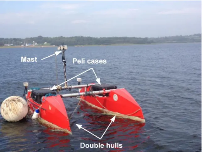
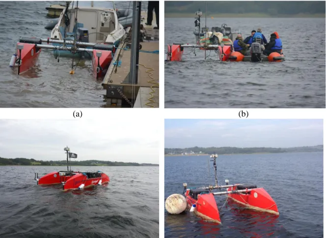
Springer USV (shown in Figure 1) is a catamaran structured vessel with the dimensions of 4.2 m in length and 2.3 m in width and a displacement of 0.6 tonnes (specific parameters are shown in Table 2). Within the vehicle, the two hull bodies are the most important component. First, the power sources - eight 12 V 135 Ah batteries - are placed within the hulls with four in each side to provide power for the electrical motors to drive two propellers to propel the vehicle.

Second, two Peli-cases with guaranteed waterproof capability are placed on two hulls to contain the Navigation, Guidance and Control (NGC) system. The NGC system consists of three digital compass units, one gyroscope and two computers running NGC algorithms. This is the core of the vehicle's navigation system and will be discussed in detail in the next section.

Thirdly, in order to establish a robust communication channel, a mast is placed in between the two hulls to carry a wireless router as well as a GPS receiver. The mast is able to

(5)

5

exchange data information between Springer and external devices as well as receive navigation information.

2.1.Vehicle dynamics

As a result of the improved stability of the catamaran structure, the motion of Springer can be reduced from the conventional six degrees of freedom to three degrees of freedom by ignoring the roll, pitch and heave motions (Motwani, 2015). Springer is steered by a differential steering mechanism by having different Revolutions Per Minute (RPM) values of two propellers. Therefore, the surge speed and the heading of the vehicle can be controlled by:

𝑛𝑐 =𝑛1+𝑛₂ 2 (1)

𝑛_𝑑 =𝑛1−𝑛2

2 (2)

where n1 and n2 are two propeller thrusts, nc is the common mode thrust defining USV's surge speed and nd is the differential mode thrust having the maximum value of 900 rpms.

In order to maintain the velocity of the USV, nc remains constant for most of time except the time period when Springer is approaching closely to waypoints. The dynamic model of

Springer was calculated from system identification (SI) process using the data obtained from the real trails conducted at Roadford Lake, Devon, UK (Naeem, et al, 2012(b)). The system dynamics is a linear second-order single-input single-output system and can be expressed in the state space form as (Motwani et al., (2013)):

𝑥(𝑘 + 1) = 𝐴𝑥(𝑘) + 𝐵𝑢(𝑘) (3a)

𝑦(𝑘) = 𝐶𝑥(𝑘) + 𝐷𝑢(𝑘) (3b)

(6)

6 𝐴 = [1.002 0 0 0.9945] (4a) 𝐵 = [ 6.354 × 10−6 −4.699 × 10−6] (4b) 𝐶 = [34.13 15.11] (4c) 𝐷 = [0] (4d)

where 𝑢(𝑘) represents the differential thrust input in rpm and 𝑦(𝑘) is the heading angle in radius. It should be noted that the sway motion is ignored for simplicity.

2.2.The navigation guidance and control (NGC) system of Springer

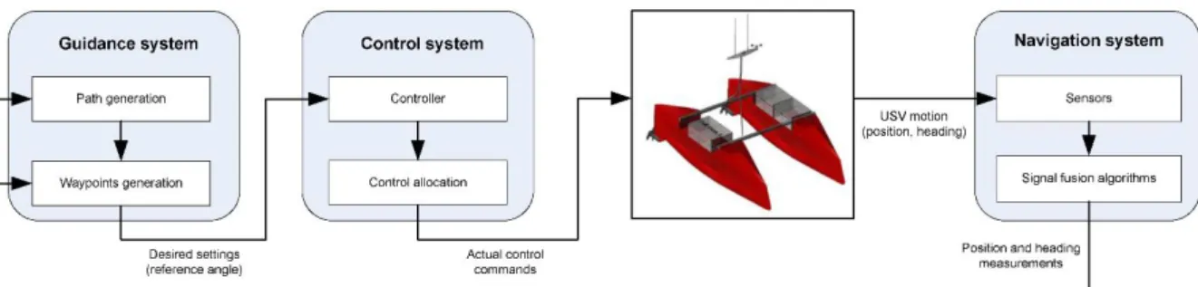
The NGC system of Springer has been systematically represented in Figure 2. It consists of three different systems namely the Guidance system, the Navigation system and the Control system. Springer perceives its surrounding environment using the Navigation system, which obtains navigation information using a range of different sensors such as the GPS, the Inertial Measurement Unit (IMU) and the compasses. The information is then processed using a data fusion algorithm to improve its accuracy. Based upon the sensor measurements, the Guidance system generates the desired reference heading angle for the Control system, which then calculates the actual control commands for Springer.

Currently, the Navigation system mounted on Springer is developed using three compasses along with a gyroscope to calculate instantaneous heading and a GPS combined with an IMU to localise the position as the vehicle is navigating. To improve the accuracy of the heading information as well as overcome possible sensors malfunctions, a weighted interval Kalman filter has been implemented (Motwani et al., 2013, 2014).

In terms of the Control system, the Linear Quadratic Gaussian (LQG) (Naeem et al., 2008), the Local Control Networks (LCNs) (Sharma et al., 2012) and the Model Predictive

(7)

7

Control (MPC) (Annamalai et al., 2015) have been designed in sequence and applied providing promising tracking performances in both simulation and experimental results. However, it should be noted that by analysing different controllers’ performances, the PID controller provides the most robust tracking results (Motwani, 2015) due to its advantages in correcting present control errors, compensating the accumulated errors and predicting the rate of change of error.

It is also worth noting that in the Navigation system of Springer, no path planning algorithm has been developed and integrated. Therefore, Springer is only able to carry out simple missions, i.e. tracking the manually predefined waypoints or trajectories, making the USV not fully autonomous. To improve the autonomy level of Springer and make it capable of automatically generating trajectory according to mission requirements, path planning algorithms have therefore been integrated into the NGC system of Springer. In the following sections, details will be given and discussed.

3. The fast marching method based path planning algorithm

3.1. The fast marching method

The fast marching method (FMM) was first proposed by J. Sethian in 1996 to iteratively solve the Eikonal equation to simulate the propagation of an interface (Sethian, 1996). The Eikonal equation has the form as:

|∇𝑇(𝒙)|𝑉(𝒙) = 1 (5)

where 𝑇(𝒙) is the interface arrival time at point 𝒙and 𝑉(𝒙) is the interface propagating speed. Equation 5 belongs to the partial deferential equation (PDE) and its numerical solution can be obtained via the upwind deferential method when using the FMM. The solving process of the FMM is similar to Dijkstra's method but in a continuous way. Suppose (x,y) is the point that

(8)

8

T(x,y) needs to be solved. The neighbour of (x,y) is a point set containing four elements (𝑥 +

∆𝑥, 𝑦), (𝑥 − ∆𝑥, 𝑦), (𝑥, 𝑦 + ∆𝑦),(𝑥, 𝑦 − ∆𝑦). T(x,y) can be obtained as:

𝑇₁ = min (𝑇_{(𝑥−∆𝑥,𝑦)}, 𝑇_{(𝑥+∆𝑥,𝑦)}) (6) 𝑇2 = min (𝑇(𝑥,𝑦−∆𝑦), 𝑇(𝑥,𝑦+∆𝑦)) (7) |∇𝑇_(𝑥,𝑦)| = √(𝑇(𝑥,𝑦)−𝑇1 ∆𝑥 ) 2 + (𝑇(𝑥,𝑦)−𝑇2 ∆𝑦 ) 2 (8) (𝑇(𝑥,𝑦)_∆𝑥−𝑇1)2+ (𝑇(𝑥,𝑦)_∆𝑦−𝑇2)2 = 1 (𝑉(𝑥,𝑦))2 (9)

where ∆𝑥 and ∆𝑦 are the grid spacing in x and y directions. The solution of Equation 8 is given by:

𝑇_(𝑥,𝑦) = { 𝑇₁+_𝑉1 (𝑥,𝑦), 𝑖𝑓 𝑇2 ≥ 𝑇 ≥ 𝑇1 𝑇2+_𝑉1 (𝑥,𝑦), 𝑖𝑓 𝑇1 ≥ 𝑇 ≥ 𝑇2 𝑄𝑢𝑎𝑑𝑟𝑎𝑡𝑖𝑐 𝑠𝑜𝑙𝑢𝑡𝑖𝑜𝑛 𝑜𝑓 𝐸𝑞𝑢𝑎𝑡𝑖𝑜𝑛 (8) 𝑖𝑓 𝑇 > max (𝑇₁, 𝑇₂) (10)

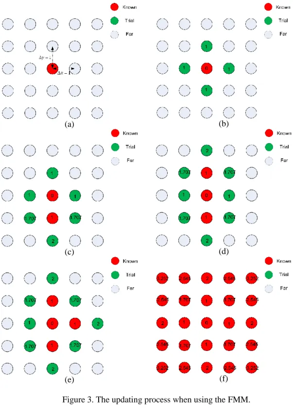
To further illustrate the FMM algorithm, a simple case representing how to update a 6*6 grid map is shown in Figure 3. Figure 3a shows the initial configuration of the algorithm with the middle point being the algorithm start point. The interface propagating speed is set to be uniform as 1 at each grip point. When the FMM is being executed, grid points are categorised into three different groups as:

 Far (marked as light blue): contains grid points with undecided arrival time value (T). In the first time step when running the FMM, all grid points except the start points belong to Far;

 Known (marked as red): contains grid points with decided arrival time values (T). Such values will not be changed when the algorithm is executed;

(9)

9

 Trial (marked as green): contains grid points with calculated arrival time values (T); however, values may be changed then the algorithm is running.

In Figure 3b, the first step time of running the FMM has been represented. The start point is currently the only Known point with T value as 0. Four neighbour points of the start point consist of the Trial set and therefore are marked as green with calculated arrival time T

as 1.

For next time step, the point with minimum arrival time cost will be first selected from the Trial set to become the new Known point; however, four neighbours have the same cost, and the point below the start point is considered as the point with the minimum cost thereby being re-marked as Known with its neighbours identified as Trial as well (shown in Figure 3c). Figure 1d and Figure 3e show how the grip map is updated by repeating such a process in time step 3 and 4, and the final updating result is represented in Figure 3f. In Figure 3f, it can be observed that the start point has the minimum arrival time 0; whereas other points’ arrival times are increasing proportionally to the distances to the start point, which forms a potential field where the potential field value is the interface arrival time with the minimum potential located at the start point.

3.2.The FMM based path planning algorithm and fast marching square method

The FMM based path planning algorithm is described in Algorithm 1. Suppose that the planning space (M) shown in Figure 4a, where the algorithm is performed on, has a representation of a binary map and is perfectly rasterised. The algorithm first reads in the M

and calculates its speed matrix (V). The speed matrix (V) is the same size as the M and defines the interface propagation speed at each point in the M. Based on the V, the FMM is executed to calculate an arrival time matrix T from the start point. The generated T (shown in Figure 4b) can be viewed as an arrival time potential field where the potential value represents local arrival

(10)

10

time of the interface, which subsequently indicates local distance to the start point if a constant speed matrix is used. Then, based upon the arrival time matrix T, the optimal path is finally searched by applying the gradient descent method (shown as the red line in Figure 4c).

Algorithm 1FMM Path_Planning Algorithm

Require: planning space (M), start point (pstart), end point (pend) 1: Calculate speed matrix V from M

2: Arrival time matrix (T) ← FMM (V, pstart, pend) 3: path ← gradient Decent (T, pstart, pend)

4: returnpath

One of the problems associated with path planning by directly using the FMM method is the generated path is too close to obstacles. Such a drawback is especially impractical for USVs, because near distance areas around obstacles (mainly islands and coastlines) are usually shallow water, which is not suitable for marine vehicles to navigate. Hence, it is important to keep the planned path a certain distance away from obstacles.

To tackle this problem, Gomez et al. 2013 has proposed a new algorithm named the fast marching square (FMS) method. The basic concept behind the FMS is to apply the conventional FMM algorithm twice but with different purposes. The FMS is represented in Algorithm 2. It first generates a safety potential map (Ms) by applying the FMM to propagate interfaces from all the points in obstacle area. Based on the Ms, the FMM is executed again from the start point to generate the final path. By using the same previous planning space, the path generated by the FMS is shown as the green trajectory in Figure 4c with increased safety.

Algorithm 2Fast_Marching_Square Algorithm

Require: planning space (M), start point (pstart), end point (pend) 1: for each point a in obstacle do

(11)

11 3: end for

4: Ms← FMM (obstaclePoints) 5: T ← FMM (Ms, pstart, pend )

6: path ← gradientDecent (T, pstart, pend ) 7: returnpath

4. The angle-guidance fast marching square method

To address the motion constraints problem of the USV when searching for a path, the FMS algorithm has been improved to a new method named the angle-guidance fast marching square (AFMS) algorithm with the specific application for USV path planning (Liu and Bucknall. 2016). Before introducing the AFMS algorithm, the basic motion equations of USV’s is explained here. Consider 〈𝑒〉 is the inertial coordinate frame and 〈𝑏〉 is the body fixed coordinate frame. Let the state of the USV relative to the 〈𝑒〉 is denoted as 𝜂 = [𝑥 𝑦 𝛼]𝑇, where x and y represent the position coordinates of the USV in the planning space and 𝛼 is the yaw angle. The surge and yaw speed of the USV is expressed with respect to 〈𝑏〉 and has the form of 𝑠 = [𝑢 𝑣 𝑟]𝑇, where u and v are surge and sway speed and r is the yaw rate. The kinematic motion of the USV can therefore be written as:

𝜂̇ = 𝐽s (11)

where

𝐽 = 𝐽(𝛼) = [cos 𝛼 − sin 𝛼 0sin 𝛼 cos 𝛼 0 0 0 1

] (12)

Normally, the USV has constant speed during operation but limited turning capability. Hence, the yaw rate is subject to the constraints of yaw boundary (𝑟_𝑚𝑎𝑥) as:

(12)

12

The pseudocode of the AFMS is shown in Algorithm 3. It uses the FMS as the base algorithm; however, before searching for a path, the AFMS calls guidanceRange function to create a guidance range (GR) upon the planning space (M) with the aim of assisting the algorithm to search the path according to the USV’s dynamics.

Algorithm 3Angle_guidance FMS Algorithm

Require: planning space (M), start point (pstart), end point (pend), heading angle (α), turning angle (θ), range radius (r)

1: range ← guidanceRange (M, r, α, pstart , θ) 2: for each point p in Obstacle sectordo 3: M (p) = 0

4: end for

5: Ms← FMS (M)

6: path ← pathgradientDecent (Ms, pstart, pend ) 7: returnpath

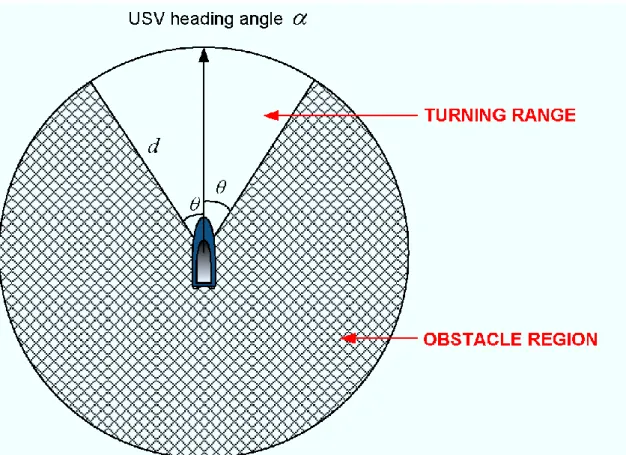
The shape of the GR is constructed graphically as shown in Figure 5. It consists of two different sectors, i.e. the Turning Range sector in white, and the Obstacle Region sector in the shaded sector. The dimensions of the Turning Range are controlled by three parameters, i.e. range distance (d), heading angle (𝛼) and turning angle (𝜃). The turning angle (𝜃) parameter is calculated according to vehicle yaw constraint as:

𝜃 = 𝑟_𝑚𝑎𝑥 ∗ ∆𝑇 (14)

where ∆𝑇 is the time step. The calculated value of 𝜃 represents the maximum turning angle that can be made by the USV during ∆𝑇, i.e. 𝜃 = 30° represents USV can only make a starboard or port side turn up to 30 degrees for one operation cycle. It should be noted that this parameter should be adjusted according to specific USV dynamics in real operation. The range distance (d) is the radius of the cone shape which is able to control the influence range affecting the path and is related to the surge speed of the USV as:

(13)

13

𝑑 = {_{𝑢 ∗ 𝑟𝑎𝑛𝑔𝑒𝑆𝑐𝑎𝑙𝑎𝑟 𝑜𝑡ℎ𝑒𝑟𝑤𝑖𝑠𝑒.}𝑑𝑚𝑖𝑛 𝑖𝑓 𝑢 < 𝑢𝑝𝑒𝑟𝑚𝑖𝑡, (15)

where 𝑑_𝑚𝑖𝑛 is the predefined minimum distance (3-4 times the vessel’s length is recommended according IMO (International Maritime Organisation) (Maritime Security Committee, 2002)) used in the case when the USV is at low speed. Enough range space will be created such that the USV can make the required turn. Also it can be observed from Equation 15 that the GR dimension increases proportionally with the USV speed. This facilitates the generated path being located more in the GR to accommodate a USV's dynamics when the USV is travelling at higher speed. The range distance (d) is also controlled by the parameter rangeScalar. This is primarily used to regulate GR range size to prevent the algorithm from generating an oversized obstacle area such that the target point will be unnecessarily blocked, which is undesirable especially in narrow passages. It is noted that both 𝑢_{𝑝𝑒𝑟𝑚𝑖𝑡} and rangeScalar should be adjust according to specific vessel’s dynamics as well as manoeuvrability. Finally, the heading angle (𝛼) represents the USV's current heading angle and determines the direction of the GR.

The weighting values inside the Turning Range sector remains the same as they are in the Planning space (M). However, since it is desired that the path should be located within the Turning Range sector making the Obstacle Range sector act like an obstacle, weighting values of the Obstacle Range are assigned as 0. By adding the GR to the original planning space, a new planning space (M) can be generated with the consideration of USV’s dynamics, upon which the FMS algorithm is employed to search for the path.

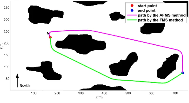
In Figure 6, paths generated by the AFMS and the FMS are compared with the AFMS’s trajectory represented in magenta and the FMS’s in green. Differing from the testing environment employed in Figure 4, a more complex area containing multiple randomly located obstacles are used in this new test. The mission start and end points are marked with red and

(14)

14

blue dots respectively. The USV has an initial heading angle of 120° with the turning angle of

30°_{and the rang distance of 15 m. To better explain the results, the zero degree has been}

defined in east direction in this case. From Figure 6(a), it can be observed that without considering the turning capability of the USV, FMS searches for the path based on the minimum distance criterion and avoids the obstacles from the bottom part of the area (shown in green line). However, a large heading change exists at the start point making the USV incapable of tracking such a trajectory. On the contrary, path provided by the AFMS stays alongside the direction of the USV’s heading and has a turning circle formed at the initial section of the trajectory to assist with the vehicle adjusting its heading. The turning circle has been formed according to the guidance of the GR as displayed in Figure 6(b). In addition, because of the influence of the GR, the AFMS’s path avoids the obstacles from upper section of the area. It should be noted that such a trajectory is calculated based upon both the minimum distance as well as the vehicle’s dynamic constraints requirements making it become a more practical solution.

5. The line-of-sight (LOS) based waypoints generator

Trajectories provided by the FMS algorithm or the AFMS algorithm have good characteristics of continuity and smoothness. If the autopilot system of a USV is capable of tracking a continuous path, there is no need to amend it. However, because Springer USV employs an autopilot system which does not track a continuous path but a series of waypoints using the line-of-sight (LOS) theory, it is required to extract informative waypoints from the path such that they can be used as reference points for the USV.

(15)

15

5.1.The LOS based guidance strategy

Because of its simplicity and ease of implementation, the LOS guidance strategy has been implemented on Springer (Naeem et al., 2003). The strategy iteratively uses the current position of the USV and the next waypoint to calculate the reference angle as:

𝜃_𝑟𝑒𝑓 = 𝑎𝑟𝑐𝑡𝑎𝑛𝑦2−𝑦1

𝑥2−𝑥1 (16)

where (x1, y1), (x2, y2) are the coordinates of USV's current position and next waypoint, respectively. The reference angle will be compared with the actual heading of Springer to generate heading control commands to adjust the movement of the vehicle.

In order to decide whether the waypoint has been reached or not, a circle of acceptance (COA) is pre-defined around each waypoint with the radius as rCOA. In each time instance, the distance, denoted as r, between the current position of the USV and next waypoint is calculated and compared with rCOA. Only when r is less than the rCOA, is it recognised that the USV has arrived at the corresponding waypoint and is able to move on to the next one.

5.2.The waypoints generator based on LOS

There is a trade-off between the number of waypoints for the USV and the tracking performance of the vehicle. Intensive waypoints along the path will create a large number of control points, which could generate a series of unwanted control outputs, thereby affecting the USV's tracking performance. However, if there are not enough waypoints placed on the path, especially on the turning arcs, a large heading angle change will occur during the transition from straight line to the circle arc. A jump in the desired yaw rate will thus be experienced, which is difficult for the autopilot to cope with.

Hence, a novel waypoints-generator algorithm is proposed to obtain useful waypoints from the calculated trajectory. It consists of two main procedures: 1) generating a series of consecutive waypoints retaining the characteristics of the trajectory and 2) using a

(16)

‘waypoints-16

trimmer’ to reduce the number of waypoints on a straight path while maintaining waypoints located on arcs. For the first step, total of number of desired waypoints can be determined by:

𝑛 =𝐿𝑡𝑟𝑎𝑗𝑒𝑐𝑡𝑜𝑟𝑦

𝑑𝑖𝑛𝑡𝑒𝑟𝑣𝑎𝑙 (17)

where 𝐿_{𝑡𝑟𝑎𝑗𝑒𝑐𝑡𝑜𝑟𝑦} represents the total length of the calculated trajectory and 𝑑_{𝑖𝑛𝑡𝑒𝑟𝑣𝑎𝑙} is the distance between every two adjacent waypoints calculated as:

𝑑𝑖𝑛𝑡𝑒𝑟𝑣𝑎𝑙 = 𝑢 ∗ ∆𝑡 (18)

where u is the speed of the USV and ∆𝑡 is the sampling time step. Note that 𝑑_{𝑖𝑛𝑡𝑒𝑟𝑣𝑎𝑙} should be selected according to the specific dynamics of the USV, i.e. for a USV with high manoeuvrability, 𝑑_{𝑖𝑛𝑡𝑒𝑟𝑣𝑎𝑙} can be assigned with a relative small value as the USV is able to adjust its motion efficiently. In fact, a larger number of waypoints 𝑛 is preferred as the larger the number is, the better the trajectory characteristics can be retained especially for non-straight sections.

After the determination of the total number of waypoints, a ‘waypoint-trimmer’ is employed to refine these waypoints by following the LOS theory. The details of the ‘waypoint-trimmer’ are presented in Algorithm 4. From the start point, every three waypoints (point A, point B, point C) are selected in sequence to calculate the turning angle ∆𝜑 by using the Law of Consines as:

∆𝜑 = 𝑎𝑟𝑐𝑐𝑜𝑠𝑎2+𝑏_2𝑎𝑏2−𝑐2 (19)

where a, b and c are the sides of length of the triangle formed by point A, B and C. If point C is not visible to point A, which is expressed as:

(17)

17

where 𝜃_𝑚𝑖𝑛 is a predefined parameter having a relatively small value, a ‘straight’ line can be determined to exist between A and C then point B can be removed. If point C is visible to point A, an arc possibly exists between A and C, therefore, point B needs to be kept to maintain the shape of the trajectory.

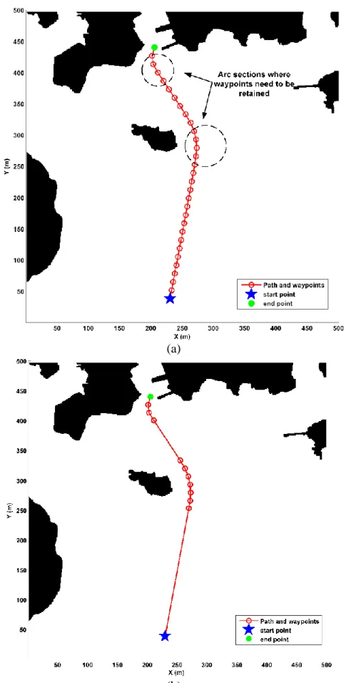
Figure 7 represents the process of waypoints generation. In Figure 7a, the result after running the first step of the waypoints-generator is displayed. It can be observed that a total number of 31 waypoints are generated and equally placed along the trajectory. The ‘waypoint-trimmer’ is then used to generate an optimal number of waypoints with the results shown in Figure 7b. It is clear that the number of waypoints has been reduced to 12 with most of them located at arc sections to preserve the continuity of the path. The advantage of using such a strategy is that optimised waypoints can be provided to ensure the USV is able to robustly follow the trajectory especially when taking complex manoeuvres such as making a turning.

Algorithm 4Waypoint trimmer Algorithm Require: waypoints (Wp), anglemin (𝜃_𝑚𝑖𝑛) 1: 𝑞_𝐴 ← 𝑊_{𝑝_𝑠𝑡𝑎𝑟𝑡} 2: 𝑞_𝐵 ← 𝑞_𝐴. 𝑛𝑒𝑥𝑡 3: 𝑞_𝐶 ← 𝑞_𝐵. 𝑛𝑒𝑥𝑡 4: while 𝑞_𝐶≠ 𝑊_{𝑝_𝑔𝑜𝑎𝑙} do 5: ∆𝜙 = 𝜙_𝐴𝐵− 𝜙_𝐵𝐶 6: ifΔ𝜙 ≤ 𝜃𝑚𝑖𝑛 then 7: Wp.remove(qB) 8: else 9: 𝑞_𝐴 ← 𝑞_𝐵 10: end if 11: 𝑞_𝐵 ← 𝑞_𝐶 12: 𝑞_𝐵 ← 𝑞_𝐶. 𝑛𝑒𝑥𝑡 13: end while 14: returnWp

(18)

18

6. The integration of the path planning algorithm with NGC system of Springer USV

To improve the autonomy level of Springer, the designed path planning algorithm has been integrated with the NGC system making the vehicle have the capability of autonomous accomplish the mission by simply knowing the mission start and end points. A three-level system has been developed including the planning level, the control level and the hardware level, which are shown in Figure 8.

Before the mission commences, the planning level is first executed based on information such as the mission environment (free and obstacle spaces) and mission requirements (the start and end points). The path planning module works out the collision-free trajectory and calculates the waypoints by using the LOS based waypoints generator. Then, the generated waypoints are transmitted to the control level, which is mainly the NGC system of

Springer, to start the mission.

By referring to the obtained waypoints, Springer employs the PID controller to track the trajectory, and the tracking performances are iteratively monitored by a sensor suite. The sensor suite consists of a single low cost gyroscopic unit and three independent compasses to estimate the actual heading of the vehicle. In addition, the IMU-GPS combined unit is used to measure the position information for Springer. The measured information will be fed back to the navigation module in the NGC system, where robust Kalman filter technology (or the Interval Kalman Filter) is used to fuse the measurements and provide accurate navigation information to improve the tracking performance (Motwani et al (2015). The refined heading angle is then compared with the reference angle to calculate the error value, which will be used as the control input to accordingly adjust vehicle’s navigation for next operation.

(19)

19 7. System validations on Springer

7.1.Full-scale experiments on Springer

A full-scale experiment was undertaken on the Roadford Lake, Devon, UK, 17-18 September 2014. The aim of the experiment was to test the integration of the FMS based path planning algorithm and the NGC system of Springer such that complete USV autonomous navigation can be achieved.

The experiment area is shown in Figure 9a with the testing area indicated by the white dashed circle. In order to validate the collision avoidance capability of Springer, a virtual obstacle has been added to the binary map of the Roadford Lake represented in Figure 9b. In Figure 10, four snapshots of different stages during the experiment are represented as: 1) USV about to be launched from the pier (Figure 10a), 2) USV being towed by human operators (Figure 10b), 3) USV in operation of tracking virtual waypoints (Figure 10c) and 4) USV reaching the target point (Figure 10d).

Experimental results are presented in Figure 11. The mission start point is waypoint 2; whereas, Springer was launched from waypoint 1. A total number of 5 waypoints (excluding the start and end points) have been generated for Springer with their GPS coordinates listed in Table 3. In Figure 11a, it can be observed that waypoints are located away from the obstacle with average deviation distance around 100 m. Such a distance is able to guarantee the safety of the vehicle throughout the operation.

The tracking performance of Springer is plotted as the blue line in Figure 11a. Good tracking results can be observed from waypoint 3 towards the end point as the small deviations occur between the blue line and the planned path (dashed black line). From the control perspective (in Figure 11b), it can also be demonstrated that generated waypoints are achievable for the autopilot of Springer to track. From time step 150 the true heading angle (in

(20)

20

red) of the USV corresponds well with the reference angle (in blue), which proves that a correct tracking is taken by Springer.

However, large deviation exists between waypoint 2 and waypoint 3. The primary reason for this is the generated path does not consider the heading of Springer when it passes waypoint 2. The reference angle at this moment makes a significant change from 250° to around 175°, which is shown in Figure 11c at time step 50. Such a large heading angle difference is impossible for the USV to cope with in such a short time period. It takes around 150 time steps for Springer to adjust its heading and accomplishes it at waypoint 3.

Therefore, the importance of the heading of the vehicle when the path is planned can be clearly demonstrated from this case and the AFMS algorithm provides an alternative algorithm for Springer. Unfortunately, due to the limited experimental time, the full-scale test of the AFMS on Springer could not able to be conducted. However, simulations based on the true dynamics of Springer of the AFMS were run, which will be discussed in next section.

7.2.Simulations based on the dynamics of Springer

In this section, simulation results of the proposed algorithms are presented and analysed with the simulation area shown in Figure 12. During the real trial, Springer is normally launched from the pier and starts the mission in the middle of the lake. Therefore, in this test, the mission start point has been selected a certain distance away from the pier (marked with red start in Figure 9), and the end point is located above it.

Two ‘islands’ are located in the area shown in Figure 13. The coordinates of start and end points are (445, 330) and (416, 650) marked as red and green points. The initial heading angle of Springer is 180° represented by the black arrow in Figure 13. Other simulation parameters including USV velocity and surface currents velocity are listed in Table 4.

Paths generated by the FMS and the AFMS are plotted and compared in Figure 13. They are represented in blue and in magenta with corresponding waypoints. It is evident that

(21)

21

path in magenta (generated by the FMS) does not consider the initial heading and directly avoids two obstacles from the right side to pursue the shortest distance. In contrast, the AFMS path can be followed within the constraints of Springer's dynamics and initial heading angle as it was planned in accordance with vehicle's initial heading angle and motion constraints. After a different path having been planned, the path passes in between the two ‘islands’ to seek the minimum path distance.

The tracking performance of Springer by following these two different paths are represented in Figure 14 and Figure 15. In Figure 14a and Figure 15a, each waypoint is marked as ‘+’ with a circle around it representing the COA. According to the accuracy of the localisation of the USV, the radius of the COA is set as 4m. When the USV is tracking each waypoint, as long as Springer enters into the COA, it is acknowledged that the corresponding waypoint has been reached so the vehicle can transit to the next waypoint.

The simulated trajectories taken by Springer are plotted as blue lines. From Figure 14a, it can be observed that Springer accurately arrives at each waypoint by entering the COA circle, which proves that the path can be tracked. However, when following the waypoints generated from the FMS path, the performance is less precise. In Figure 15a, large deviations occur during the initial stages and several waypoints have been missed by Springer. The reason for this is

Springer has to adjust its heading at the beginning to turn towards the reference direction determined by the waypoints. This is shown from the comparison between Figure 14b and Figure 15b, which record the real-time control input and heading angle. In Figure 15b, between time steps 0 and 200, the control inputs vary dramatically between positive and negative maximum values. The USV takes alternate full-rudder starboard or port side turnings as a result of trying to attain a path produced with no consideration to Springer's dynamic capability and the limitations of its autopilot control have been exceeded; whereas in Figure 14b, less serve control inputs are required meaning Springer is easier to track.

(22)

22

To quantitatively assess the tracking performance, the distance error of each vehicle's instantaneous position at time k to the desired trajectory is recorded. Such an error value can be measured using the Heron's formula as:

𝑑(𝑘) =√(𝑎+𝑏+𝑐)(−𝑎+𝑏+𝑐)(𝑎−𝑏+𝑐)(𝑎+𝑏−𝑐)_2𝑎 (21)

where a, b, and c are the sides of the triangle, which is formed by the USV's instantaneous position and two adjacent waypoints, as shown in Figure 16. Error values by following two different paths are plotted in Figure 14c and Figure 15c. The highest error for the FMS path is 20 m, which happens at time step 25. Such a deviation from the desired trajectory is especially of risk if the vehicle is navigating in a constrained area, where potential collisions could happen. In terms of the distance error for the AFMS, it can be well kept under 4 m, which is sufficient to maintain the margin of safety.

Further comparison of Figure 14c and Figure 15c indicates both the AFMS and the FMS provide paths that Springer can maintain, as shown in the latter stages of the transit for FMS. From this it can be deduced that the advantage of AFMS lies in its ability to plan a path that is commensurate with the USV's dynamic characteristic throughout the whole transit as it does not provide a path beyond the capability of the USV at the outset regardless of initial heading. In effect AFMS brings strategic decision making planning to the path planning problem. AFMS becomes more advantageous as the USV's dynamic characteristics become more limited and as the initial heading of the USV deviates more from the initial heading that would be planned by FMS. Although AFMS may plan a path that is of higher cost than FMS, it would provide a low risk and feasible path for the USV while FMS could produce paths that are not practical within the environment.

(23)

23 8. Conclusion remarks

This paper has presented a novel design of an intelligent navigation system for an unmanned surface vehicle, Springer USV. The system is achieved by integrating an AFMS based path planning algorithm into the NGC module of Springer. With the assistance of the path planning algorithm, Springer can now autonomously generate optimal collision free trajectory based on the mission requirements, and robustly follow the path to accomplish tasks. Simulations results have shown that the AFMS based path planning algorithm is superior to the FMS based one as the AFMS is able to search the path according to the vehicle’s dynamics constraints especially the turning capability while the advantages of the FMS can be largely retained.

Acknowledgment

This work is supported by the ACCeSS group.The Atlantic Centre for the innovative design and Control of Small Ships (ACCeSS) is an ONR-NNRNE programme with Grant no. N0014 10-1-0652, the group consists of universities and industry partners conducting small ships related researches. The authors are also grateful for Autonomous Marine Systems Research Group, Plymouth University and Professor Robert Sutton for helping undertake the experiments and providing the dynamic model of Springer USV.

References

Annamalai, A., Sutton, R., Yang, C., Culverhouse, P., and Sharma, S. 2015. Robust adaptive control of an uninhabited surface vehicle. Journal of Intelligent & Robotic Systems, 78(2):319– 338.

Caccia, M., Bono, R., Bruzzone, G., Spirandelli, E., Veruggio, G., Stortini, A., and Capodaglio, G. 2005. Sampling sea surfaces with sesamo: an autonomous craft for the study of sea-air interactions. Robotics & Automation Magazine, IEEE, 12(3):95– 105.

Curcio, J., Leonard, J., and Patrikalakis, A. 2005. Scout-a low cost autonomous surface platform for research in cooperative autonomy. In Proceedings of MTS/IEEE OCEANS Conference, 2005, pages 725–729.

Garrido, S., Moreno, L., and Lima, P. U. 2011. Robot formation motion planning using fast marching. Robotics and Autonomous Systems, 59(9):675–683.

(24)

24

Gomez, J. V., Lumbier, A., Garrido, S., and Moreno, L. 2013. Planning robot formations with fast marching square including uncertainty conditions. Robotics and Autonomous Systems, 61(2):137–152.

Liu, Y, Song, R, and Bucknall, R. 2015. A practical path planning and navigation algorithm for an unmanned surface vehicle using the fast marching algorithm. OCEANS 2015-Genova. Liu, Y. and Bucknall, R. 2016. The angle guidance path planning algorithms for unmanned surface vehicle formations by using the fast marching method. Applied Ocean Research, 59: 327-344. DOI: 10.1016/j.apor.2016.06.013

Manley, J. E. 1997. Development of the autonomous surface craft aces. In Proceedings of MTS/IEEE Conference OCEANS, 1997, volume 2, pages 827–832.

Martins, A., Almeida, J., Ferreira, H., Silva, H., Dias, N., Dias, A., Almeida, C., and Silva, E. 2007. Autonomous surface vehicle docking manoeuvre with visual information. In 2007 IEEE International Conference on Robotics and Automation, pages 4994–4999.

Maritime Security Committee, 2002. Standards for Ship Manoeuvrability. URL: http://legacy.sname.org/committees/tech_ops/O44/imo/maneuverstandards.pdf

Motwani, A., Sharma, S., Sutton, R., and Culverhouse, P. 2013. Interval kalman filtering in navigation system design for an uninhabited surface vehicle. Journal of Navigation, 66(05):639–652.

Motwani, A., Sharma, S. K., Sutton, R., and Culverhouse, P. 2014. Application of artificial neural networks to weighted interval kalman filtering. Proceedings of the Institution of Mechanical Engineers, Part I: Journal of Systems and Control Engineering, 228 (5):267–277. Motwani, A. 2015. Interval Kalman Filtering Techniques for Unmanned Surface Vehicle Navigation. PhD thesis, Plymouth University.

Motwani, A. Liu, W., Sharma, S. k., Sutton, R., and Bucknall,. R. 2015. An interval Kalman filter–based fuzzy multi-sensor fusion approach for fault-tolerant heading estimation of an autonomous surface vehicle. Proceedings of the Institution of Mechanical Engineers, Part M: Journal of Engineering for the Maritime Environment. 1475090215596180.

Naeem,W., Sutton, R., Ahmad, S., and Burns, R. 2003. A review of guidance laws applicable to unmanned underwater vehicles. Journal of Navigation, 56(01):15–29.

Naeem,W., Xu, T., Sutton, R., and Tiano, A. 2008. The design of a navigation, guidance, and control system for an unmanned surface vehicle for environmental monitoring. Proceedings of the Institution of Mechanical Engineers, Part M: Journal of Engineering for the Maritime Environment, 222(2):67–79.

Naeem, W., Sutton, R., and Xu, T. 2012b. An integrated multi-sensor data fusion algorithm and autopilot implementation in an uninhabited surface craft. Ocean Engineering, 39:43–52. Naeem, W., Irwin, G. W., & Yang, A. 2012. COLREGs-based collision avoidance strategies for unmanned surface vehicles. Mechatronics, 22(6): 669-678.

(25)

25

Sethian, J. A. 1996. A fast marching level set method for monotonically advancing fronts. Proceedings of the National Academy of Sciences, 93(4):1591–1595.

Sharma, S., Naeem, W., and Sutton, R. 2012. An autopilot based on a local control network design for an unmanned surface vehicle. Journal of Navigation, 65(02):281–301.

Sutton, R., Sharma, S., and Xao, T. 2011. Adaptive navigation systems for an unmanned surface vehicle. Journal of Marine Engineering & Technology, 10(3):3–20.

(26)

26

(27)

27

(28)

28

(a) (b)

(c) (d)

(e) (f)

(29)

29

(a) (b)

(c)

Figure 4. (a) The grid map. (b) Potential field generated by using the FMM. Potential value at each point represents the local distance to the start point. Higher the potential is, longer the distance to the start point. (c) Path generated by using the FMM (red line) and the FMS (green line).

(30)

30

(31)

31 (a)

(b)

Figure 6. Comparison of trajectories generated by the AFMS and the FMS. (a) The generated trajectories of the AFMS and the FMS in a cluttered environment. (b) The associated

(32)

32 (a)

(b)

Figure 7. Comparison of waypoints with and without using the ‘waypoints-trimmer’. (a) Path with unrefined waypoints. (b) Path with optimal number of waypoints.

(33)

33

(34)

34

(a) (b)

Figure 9. The experiments on Roadford Lake, UK. (a) The experiment area, Roadford Lake, Devon, UK. The testing area is indicated by the white circle. (b) The binary map of the experiment area with one virtual obstacle.

(35)

35

(a) (b)

(c) (d)

Figure 10. Experiments on Springer USV. (a) USV launching from the pier. (b) USV towing. (c) USV in operation tracking the waypoints. (d) USV arriving at the destination.

(36)

36 (a)

(37)

37 (c)

Figure 11. Experiment results of tracking waypoints generated by the FMM. (a) Trajectory taken by Springer, (b) comparison between the reference heading angle and the true heading angle, (c) control inputs.

(38)

38

(39)

39

(40)

40 (a)

(41)

41 (c)

Figure 14. The tracking performance of Springer when following the path generated by the AFMS.

(42)

42 (a)

(43)