Copyright and use of this thesis
This thesis must be used in accordance with the provisions of the Copyright Act 1968.Reproduction of material protected by copyright may be an infringement of copyright and
copyright owners may be entitled to take legal action against persons who infringe their copyright.
Section 51 (2) of the Copyright Act permits an authorized officer of a university library or archives to provide a copy (by communication or otherwise) of an unpublished thesis kept in the library or archives, to a person who satisfies the authorized officer that he or she requires the reproduction for the purposes of research or study.
The Copyright Act grants the creator of a work a number of moral rights, specifically the right of attribution, the right against false attribution and the right of integrity.
You may infringe the author’s moral rights if you: - fail to acknowledge the author of this thesis if
you quote sections from the work - attribute this thesis to another author - subject this thesis to derogatory treatment
which may prejudice the author’s reputation For further information contact the
University’s Copyright Service.
ROBUST AND ADVERSARIAL DATA
MINING
A thesis submitted in fulfilment of the requirements for the
degree of Doctor of Philosophy in the School of Information Technologies at The University of Sydney
Fei Wang August 2015
c
Copyright by Fei Wang 2015
All Rights Reserved
Abstract
In the domain of data mining and machine learning, researchers have made significant contributions in developing algorithms handling clustering and classification problems. We develop algorithms under assumptions that are not met by previous works. (i) In adversarial learning, which is the study of machine learning techniques deployed in non-benign environments. We design an algorithm to show how a classifier should be designed to be robust against sparse adversarial attacks. Our main insight is that sparse
feature attacks are best defended by designing classifiers which use`1regularizers. (ii)
The different properties between`1 (Lasso) and`2(Tikhonov or Ridge) regularization
has been studied extensively. However, given a data set, principle to follow in terms of choosing the suitable regularizer is yet to be developed. We use mathematical properties of the two regularization methods followed by detailed experimentation to understand their impact based on four characteristics. (iii) The identification of anomalies is an inherent component of knowledge discovery. In lots of cases, the number of features of a data set can be traced to a much smaller set of features. We claim that algorithms applied in a latent space are more robust. This can lead to more accurate results, and potentially provide a natural medium to explain and describe outliers. (iv) We also apply data mining techniques on health care industry. In a lot cases, health insurance companies cover unnecessary costs carried out by healthcare providers. The potential adversarial behaviors of surgeon physicians are addressed. We describe a specific con-text of private healthcare in Australia and describe our social network based approach (applied to health insurance claims) to understand the nature of collaboration among doctors treating hospital inpatients and explore the impact of collaboration on cost and quality of care. (v) We further develop models that predict the behaviors of orthopedic surgeons in regard to surgery type and use of prosthetic device. An important feature of these models is that they can not only predict the behaviors of surgeons but also provide explanation for the predictions.
Statement of Originality
I hereby certify that this thesis contains no material that has been accepted for the award of any other degree in any university or other institution.
————————————————————-Fei Wang
March 31, 2015
Acknowledgements
Firstly, I would like to give thanks to my dear supervisor, Professor Sanjay Chawla, for his essential support and guidance during my research . The achievements during my three years research has been an outcome by his invaluable and indispensable expertise, stimulation and encouragement. I would also like to thank my industry supervisor Uma Srinivasan and Bavani Arunasalam for their invaluable advice and provision of domain knowledge, and my associate supervisor, Dr. Anastasios Viglas, for his purport to my comfortable research environment.
I would like to thank Capital Markets CRC for providing me with a PhD scholarship.
Finally, I want to thank my parents for their infinite support throughout my life overseas.
Publications
This thesis has led to the following publications:
1. Wang, Fei, Sanjay Chawla, and Didi Surian. “Latent outlier detection and the low precision problem.” Proceedings of the ACM SIGKDD Workshop on Outlier Detection and Description. ACM, 2013.
2. Wang, Fei, Sanjay Chawla, and Wei Liu. “Tikhonov or Lasso Regularization: Which Is Better and When.” Tools with Artificial Intelligence (ICTAI), 2013 IEEE 25th International Conference on. IEEE, 2013.
3. Wang, Fei, Uma Srinivasan, Shahadat Uddin, and Sanjay Chawla. “Application of Network Analysis on Healthcare.” Advances in Social Networks Analysis and Mining (ASONAM), 2014 IEEE/ACM International Conference on. IEEE, 2014. 4. Wang, Fei, Wei Liu, and Sanjay Chawla. “On Sparse Feature Attacks in Adver-sarial Learning.” IEEE International Conference on Data Mining series (ICDM), 2014.
Contents
Abstract iii
Statement of Originality iv
Acknowledgements v
Publications vi
List of Tables xiii
List of Figures xvi
1 Introduction 1
1.1 Contributions of this Thesis . . . 3
1.2 Organization . . . 4
2 Background 5 2.1 Related Literature . . . 5
2.1.1 Algorithm Oriented . . . 5
2.1.2 Healthcare Oriented . . . 7
2.2 Key Concepts and Evaluation Metrics . . . 9
2.2.1 Non Zero-sum Game . . . 9
2.2.2 Logistic regression . . . 11 2.2.3 Regularizations . . . 13 2.2.4 Network concepts . . . 15 2.2.5 Confusion Matrix . . . 18 2.2.6 ROC . . . 19 vii
3 Adversarial Learning 20
3.1 Introduction . . . 20
3.2 Solving The Non Zero-sum Game . . . 23
3.2.1 Lasso and robust regression . . . 24
3.2.2 Robust regression and minimum budget of adversary . . . 26
3.2.3 Evaluation of regularizer . . . 27
3.3 Experiments . . . 27
3.3.1 Data set . . . 28
3.3.1.1 (USPS) Digit Image data set . . . 28
3.3.1.2 (Malinglist) Mailinglist data set . . . 28
3.3.1.3 Spambase data set . . . 28
3.3.2 Why sparse feature attack for the adversary? . . . 29
3.3.2.1 A more realistic behavior . . . 29
3.3.2.2 Leads to better classifier . . . 29
3.3.2.3 The game converges faster with less cost and feature modifications . . . 30
3.3.3 Why`1regularizer for data miner? . . . 32
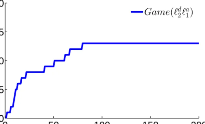
3.3.4 Evaluation of the budgetMB . . . 34
3.3.5 Evaluating logistic loss with`d2 . . . 35
3.3.6 Evaluating logistic loss with`d1 . . . 36
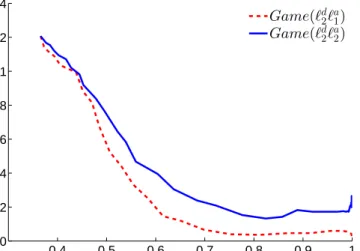
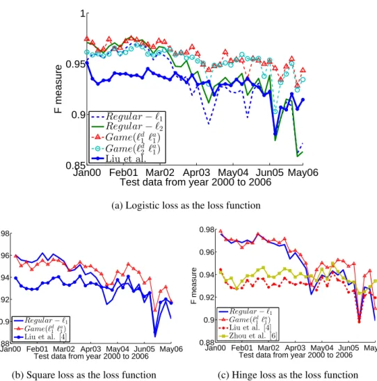
3.3.7 Comparison of`d1and`d2 on logistic loss . . . 37
3.3.8 Comparison with other methods . . . 38
3.4 Summary . . . 38
4 Tikhonov or Lasso Regularization 40 4.1 Motivation . . . 40
4.2 Contributions . . . 41
4.3 Notation and Setup . . . 42
4.4 Related Work . . . 43 4.5 Decision Map . . . 44 4.5.1 Algorithmic stability . . . 44 4.5.2 Robustness . . . 45 4.5.3 Correlation . . . 46 4.5.4 Shape . . . 48 viii
4.5.5 Decision map . . . 48
4.6 Experiments . . . 49
4.6.1 Data Sets . . . 49
4.6.2 Stability and Robustness . . . 50
4.6.3 Shape . . . 52
4.6.4 Correlation and Shape . . . 53
4.6.4.1 AllWeak . . . 54
4.6.4.2 FewStrong . . . 54
4.6.4.3 SpamBase . . . 55
4.6.4.4 WebSpam . . . 55
4.7 Summary . . . 55
5 Latent Outlier Detection 57 5.1 Introduction . . . 57
5.2 The multiple subspace view . . . 58
5.3 High-Dimensional Anomalies . . . 59
5.4 Matrix Factorization . . . 60
5.4.1 The impact of Projections . . . 61
5.4.2 Sensitivity to Outliers . . . 61
5.5 Experiments and Results . . . 63
5.5.1 Data Sets . . . 65
5.5.2 Results . . . 66
5.6 Summary . . . 71
6 Network Analysis on Healthcare 73 6.1 Introduction . . . 73
6.2 Collaboration in health care . . . 75
6.3 Surgeon Collaboration network Design . . . 76
6.3.1 Design of Collaboration Network (CN) . . . 76
6.3.2 Design of Surgeon Centric Collaboration Network (SCCN) . . . 78
6.4 Data analysis . . . 79
6.4.1 Data preparation . . . 79
6.4.1.1 Selection of admission-related variables . . . 79
6.4.1.2 Selection of network variables . . . 79 ix
6.4.1.3 Selection of Quality of Care parameters . . . 80
6.4.1.4 Data cleansing and transformation . . . 81
6.4.2 Simple linear regression . . . 81
6.4.2.1 Non network features . . . 82
6.4.2.2 Network features of SCCN . . . 83
6.4.2.3 Network features of CN . . . 83
6.4.3 Treatment analysis . . . 84
6.5 Summary . . . 85
7 Social Learning on Surgeons’ Behaviour 86 7.1 Introduction . . . 86
7.2 Background and Related Work . . . 87
7.3 Problem Definition . . . 88
7.4 Models . . . 90
7.4.1 Social Relationship Model (SRM) . . . 90
7.4.2 Positive Social Relationship Model (P-SRM) . . . 91
7.4.3 Baseline Model OMV . . . 92
7.5 Artificial Data Experiments . . . 93
7.5.1 Performance tests . . . 94
7.5.2 Sensitivity to influential index . . . 95
7.5.3 Sensitivity to network sparsity . . . 95
7.6 Hospital Data Set . . . 97
7.6.1 Data Preparation . . . 97 7.6.1.1 Surgeon networks . . . 97 7.6.1.2 Surgical procedures . . . 98 7.6.1.3 Prosthetic devices . . . 99 7.6.1.4 Observation weighting . . . 101 7.6.2 Experimental Results . . . 101 7.6.2.1 Surgical procedures . . . 101 7.6.2.2 Prosthetic devices . . . 104 7.6.2.3 Comparing results . . . 105 7.7 Summary . . . 105 x
8 Conclusions and Future Work 107
8.1 Conclusions of the Thesis . . . 107
8.2 Recommendations for Future Work . . . 109
Bibliography 110
List of Tables
2.1 Commonly used loss functions for the two players. . . 10
2.2 Representation of Classification Results via a Confusion Matrix . . . . 18
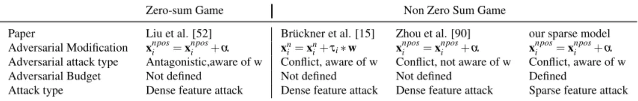
3.1 Comparisons of our sparse model with previous game theoretic models. 23
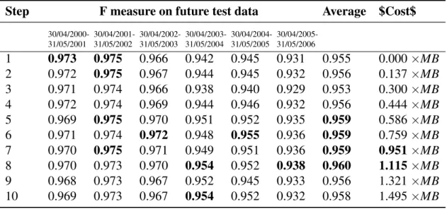
3.2 The classifier achieves best performance when theCostis close to 1×MB. 34
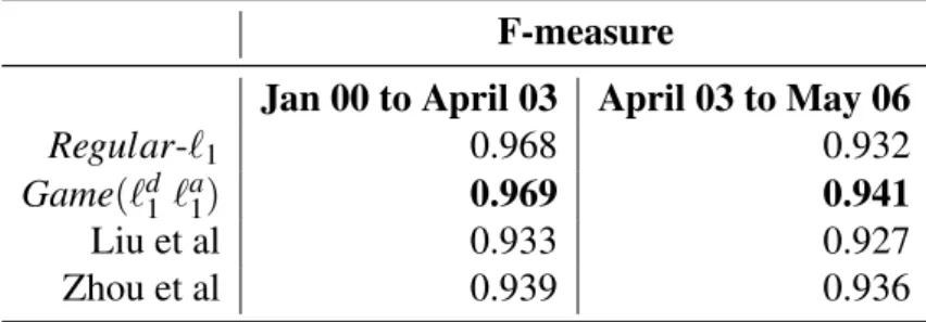
3.3 Data miner modeled with`2regularizer. Game-theoretic classifier
per-form better on data further into the future. . . 36
3.4 Sparse modelGame(`d1 `a1)achieves the best performance. . . 36
3.5 Square loss as the loss function, Game(`d1 `a1) performs best on data
further into the future. . . 38
3.6 Hinge loss as the loss function, Game(`d1 `a1) performs best on all the
future data. . . 38
4.1 Commonly used loss functions and their conjugate functions. Since
our focus is on the impact of the regularization, our results are general and are applicable to other loss functions by matching them with their
appropriate conjugate function. . . 43
4.2 Four real and three synthetically constructed data sets were used for the
experiments. More detail about the data sets is in the text. . . 50
5.1 Given the highly competitive nature of the NBA, not only are stars
out-liers, but outliers are stars! All the top five outliers are well known
leading players of NBA. . . 58
5.2 Non-Negative Factorization provides enhanced interpretation of the
meta-features. In text processing, the meta-features can be interpreted as topics, while in micro-array analysis, the meta-features are group of
correlated genes. . . 61
5.3 Precision on Spambase: DRMF, SR-NMF and R-NMF. Best values are
highlighted. . . 69
5.4 Recall on Spambase: DRMF, SR-NMF and R-NMF. Best values are highlighted. . . 69
5.5 Precision on Abstract: DRMF, SR-NMF and R-NMF. PhysicsAnomaly. 69 5.6 Recall on Abstract: DRMF, SR-NMF and R-NMF. PhysicsAnomaly. . . 70
5.7 Recision on Abstract: DRMF, SR-NMF and R-NMF. ScienceAnomaly. 70 5.8 Recall on Abstract: DRMF, SR-NMF and R-NMF. ScienceAnomaly. . . 70
5.9 Given the highly competitive nature of the NBA, not only are stars out-liers, but outliers are stars! All the top five outliers are well known leading players of NBA. . . 71
6.1 The table shows all the features we have extracted from the data and the network. . . 81
6.2 Table explores the impact of all non-network attributes on quality of cares (i.e. LoS, Medical cost) . . . 82
6.3 The table explores the impact of the network structure around a spe-cialist (based on SCCN) on quality of cares (i.e. LoS, Complication rate and Medical cost). . . 82
6.4 The table shows the impact of network position of individual specialist in the complete network (CN) on quality of cares (i.e. LoS, Complica-tion rate). . . 82
6.5 Average LoS and percentage of admissions of the four knee categories. 84 6.6 We can observe that, in terms of all the four treatment types, group B consistently has a lower Average LoS compared to group A and also the whole data set as shown in Table 6.5. . . 84
7.1 Adjacency matrices based on networks in Figure 7.1. . . 89
7.2 The three networks used in the hospital data experiments. . . 98
7.3 MBS code description . . . 103
7.4 Prosthesis code description . . . 105
List of Figures
2.1 Illustration of a star, a line, a circle and a complete graph. . . 15
3.1 Sparse feature attack identifies the most significant feature that
distin-guishes “7” and “9”, and keeps most original pixels intact after the attack. 21
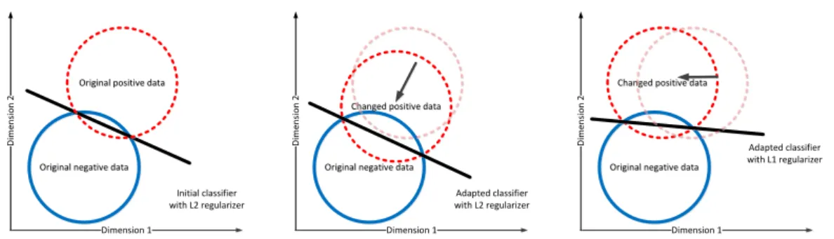
3.2 Adversarial classification problems in two dimensional space. Each
cir-cle represents a group of data in the same category. Straight lines
rep-resent the classification boundaries. . . 22
3.3 The graph demonstrating the merits of using a game-theoretic classifier. 25
3.4 When adversary is assumed to apply sparse feature attack, the learned
classifier has better performance. . . 30
3.5 The game with sparse feature attack reaches a stable state much faster
compared to a dense attack and is associated with lower cost. . . 30
3.6 The game with sparse feature attack identify and modifies a limited
number of features, in this case, 13 out of 50 features. . . 31
3.7 Regular-`1is more robust in both F-measure and AUC value compared
toRegular-`2. . . 34
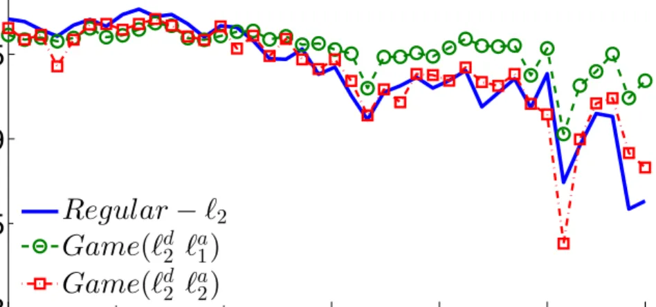
3.8 Game(`d2 `a1) model outperforms Regular-`2 classifier in terms of
F-measure data in further into the future. . . 35
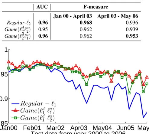
3.9 Game(`d1`a2)andGame(`d1`a1)both outperform the initial classifier with
`1regularizer in terms of both F-measure. . . 36
3.10 Sparse modelGame(`d1 `a1)has the best F-measure results on data
fur-ther into the future. . . 37
4.1 A map [left to right] to guide practitioners in their choice of a
regular-izer for supervised learning tasks . . . 41
4.2 (c) shows the Exchange rate of AUDUSD in six years. One can notice that the data is rather not stable. (a),(b),(d) clearly show that distribution
results of `2 regularizer has lower standard deviation and thus more
stable, . . . 52
4.3 Robustness: The figures indicate that distribution results of`1
regular-izer has lower standard deviation and thus more robust. . . 52
4.4 Shape: The figures indicate that`1regularization ignores the irrelevant
features with much fewer training samples. . . 53
4.5 AUC value of four data sets. For each data set we have four plots, `1
and `2 regularization and one is with x-axis as the number of training
samples and one is with x-axis as the value ofλ. . . 56
5.1 An example to explain the difference between intrinsic and ambient
dimension. Samples from the 698-image Yale face data. Each 64 x 64 is a point in a 4,096 dimensional space. However the set of images live in a three dimension set. The bottom right image is added as the
transpose of the top left image and is an outlier. . . 60
5.2 The figure shows the impact of projections of outliers in a lower
dimen-sional space. Data points 1 and 2 remain outliers after projection, while
data point 3 is mixed with normal after the projection [41]. . . 62
5.3 R-NMF is substantially more robust against the presence of outliers in
the data compared to standard O-NMF. . . 66
5.4 R-NMF converges with all given settings ofk. As the dimension of the
subspace (k) increases, residual of R-NMF algorithm goes down. . . 67
5.5 Average Run time R-NMF on Spambase data set: (Left) k = 1, (Middle)
k = 2, (Right) k = 3. As the number of outliers increases, the run time
for R-NMF decreases. The values here are the average values for all
iterations. . . 68
6.1 The tripartite graph represent the collaboration between three types
of providers: surgeons (red), anaesthetists (blue) and assistants (light blue). The edge thickness is modeled as the number of collaborating claims by two types of providers. The size of the node is modeled as
the medical charge of the provider. . . 77
6.2 Two SCCN graphs with hospital represented by a building icon. . . 78
6.3 Surgeon node with Number of triangle as 3 . . . 80
7.1 Networks defined in terms of two different relationships. . . 89
7.2 The four performance measures for the the three algorithms on the SRM
data (a) and the P-SRM data (b). As expected the SRM model outper-forms both the OMV and P-SRM when applied to the SRM data and the P-SRM outperforms OMV and the SRM when applied to the P-SRM
data. . . 95
7.3 As the influential indexSof test samples increase, the performance of
SRM and P-SRM decreases, however SRM and P-SRM still
outper-forms the baseline method OMV. . . 96
7.4 SRM has the best performance, while OMV has the least scores when
varying values of sparsity of networks. We also notice that SRM has
the most stable and robust performance. . . 97
7.5 Distribution of surgical procedures performed in the hospital data. . . . 100
7.6 Distribution of prosthetic devices in the hospital data. . . 100
7.7 The four performance measures for the the three algorithms on the MBS
codes (a) and the prosthesis data (b). . . 102
7.8 As expected the influential indices estimated by the SRM model show
that the surgeon network contains a very small number of surgeon “lead-ers”, with high influential indices. The overall sparsity of the indices is 13%, meaning that only 13% of the influential indices are significantly different from zero. . . 103
7.9 Comparative workload distribution of most influential surgeons in the
three networks. . . 104
Chapter 1
Introduction
With the technological advances during recent years, data scientists are able to obtain data that are significantly larger, complex and in real time with relatively minimal effort. Thus, the era of big data has arrived. Besides the need to modify traditional data mining techniques in order to be scalable to the ever larger data sets, there is a requirement to relax traditional assumptions associated with data mining tasks. For example, in many situations practical large scale systems which deploy classifiers, e.g., spam filters are subject to adversarial reaction. Thus there is a need to design algorithms which are ro-bust against adversarial attack. The classification problem is one of the most intensively studied problem in machine learning and data mining. A fundamental assumption un-derlying most classification problems is that the training and the test data are generated from the same underlying probability distribution. This assumption underpins both the research and applied “prediction industry.”
However there are at least two scenarios where the assumption does not hold in practice.
• Concept drift: In some scenarios, data naturally evolves with time. For example,
suppose a credit card scoring model was built during “good” economic times. Then it is natural to expect that the performance of this model is likely to deteri-orate during a recession.
• Adversarial attack: In some other situations an adversarial attack has been
ob-served against the classifier. For example, spam filters (which are classifiers) routinely have to be retrained as an adversarial reaction causes their performance to deteriorate.
2 CHAPTER 1. INTRODUCTION
Furthermore, the role of data mining and machine learning is not just inference but also discovery and the outlier detection methods can also be an important tool for dis-covering potentially new and useful patterns in data. In fact it has been often stated that new scientific paradigms are often triggered by the need to explain outliers [47]. The availability of large and ever increasing data sets, across a wide spectrum of domains, provides an opportunity to actively identify outliers with the hope of making new dis-coveries. The obvious dilemma in outlier detection is whether the discovered outliers are an artifact of the measurement device or indicative of something more fundamental. Thus the need is not only to design algorithms to identify complex outliers but also provide a framework where they can be described and explained.
The adversarial effect can also be found in healthcare domain. To be able to identify and explain the potential adversary of healthcare providers could save insurance compa-nies billions of dolors. Social network analysis is commonly used to study relationships between individuals and communities as they interact with each other. Analysing Face-book connections is one such classic example. The textFace-book by Easley and Kleinberg [27] offers deep insight into the complexity of a connected world. More interesting and novel applications of network theory are reported in specialised domains [1, 2]. In the healthcare domain, social network analysis has been used in different settings, for ex-ample to study collaboration among healthcare professionals in specific healthcare en-vironments, to understand the impact of team structure on quality of care [80, 48, 10]. In this dissertation we describe our approach of applying social network analysis in the domain of health insurance claims. In particular, we use data from health insur-ance claims to design network-based models of collaboration among medical providers and analyse the impact of social networks and their underlying network structures, to discover provider communities and analyse the topology of the emerging community structure (of surgeons, anaesthetists and assistant surgeons) on treatment outcomes for patients who undergo specific category of surgeries, for example knee surgeries.
The increased demand for high quality and cost-effective delivery of healthcare ser-vices, brings the entire healthcare sector under close scrutiny. Medical organizations such as the American College of Physicians [63] have started evaluating the feasibility of medical interventions for clinicians in terms of long term benefits, potential harms and monetary considerations. Decisions related to the adoption or discontinuation of different types of medical interventions are often a collaborative process. Providers employed by the same hospitals, who share common patients as well as the working
1.1. CONTRIBUTIONS OF THIS THESIS 3 environment, may influence each other, and social relationships can become a powerful driver of learning and innovation, as often assumed in social learning theory [7].
1.1
Contributions of this Thesis
In this thesis, we present our recent research on designing robust methods for handling adversarial situations. Specifically, our main contributions are:
1. We claim in adversarial learning the aim of an adversary is not just to subvert a classifier but carry out data transformation in a way such that spam continues to appear like spam to the user as much as possible. We demonstrate that an adversary achieves this objective by carrying out a sparse feature attack. We design an algorithm to show how a classifier should be designed to be robust against sparse adversarial attacks. Our main insight is that sparse feature attacks
are best defended by designing classifiers which use`1regularizers.
2. We use mathematical properties of the `1 (Lasso) and `2 (Tikhonov or Ridge)
regularization methods followed by detailed experimentation to understand their impact based on four characteristics: non-stationarity of the data generating pro-cess; level of noise in the data sensing mechanism; degree of correlation between dependent and independent variables and the shape of the data set. The practical outcome of our research is that it can serve as a guide for practitioners of large scale data mining and machine learning tools in their day-to-day practice.
3. We claim that algorithms for discovery of outliers in a latent space will not only lead to more accurate results but potentially provide a natural medium to explain and describe outliers. Specifically, we propose combining Non-Negative Matrix Factorization (NMF) with subspace analysis to discover and interpret outliers. We report on preliminary work towards such an approach.
4. We describe a specific context of private healthcare in Australia and describe our social network analysis (SNA) based approach (applied to health insurance claims) to understand the nature of collaboration among doctors treating hospital inpatients and explore the impact of collaboration on cost and quality of care. In particular, we use network analysis to (a) design collaboration models among
4 CHAPTER 1. INTRODUCTION
surgeons, anaesthetists and assistants who work together while treating patients admitted for specific types of treatments (b) identify and extract specific types of network topologies that indicate the way doctors collaborate while treating patients and (c) analyse the impact of these topologies on cost and quality of care provided to those patients.
5. We develop models that predict the behaviors of orthopedic surgeons in regard to surgery type and use of prosthetic device. The models utilize data on past practicing behaviours and take in account the social relationships existing among surgeons, anaesthetists and assistants. We refer to the models as the Social Re-lationship Model (SRM) and Positive Social ReRe-lationship Model (P-SRM). An important feature of these models is that they can not only predict the behaviors of surgeons but they can also provide an explanation for the predictions. Experi-mental results on both artificial and real hospital data sets show that our proposed models outperform the baseline model Online Majority Vote (OMV).
1.2
Organization
The remainder of this thesis is organized as follows. In Chapter 2 we review related literature, key concepts and evaluation metrics used in this thesis. Chapter 3, 4 and 5 respectively depict how we can build more robust models based on existing classifica-tion, regularizaclassifica-tion, and outlier detection algorithms etc. Chapter 6 describe our social network based approach (applied to health insurance claims) to understand the nature of collaboration among doctors treating hospital inpatients and explore the impact of collaboration on cost and quality of care. In chapter 7, we develop models that predict the behaviors of orthopedic surgeons in regard to surgery type and use of prosthetic devices. We conclude in Chapter 8 with directions for future work.
Chapter 2
Background
In this chapter, we present related literature, key concepts and evaluation metrics. The evaluation metrics introduced in this chapter are used throughout the thesis.
2.1
Related Literature
We review related work from two perspectives. We first overview the relevant algorith-mic literature on adversarial learning and robust classification. As one of the important application domain is health-care analysis, we review important parts of the domain literature to put our work in an appropriate context.
2.1.1
Algorithm Oriented
Adversarial Classification
Dalvi et al. [24] modelled the interaction between a data miner and an adversary as a game between two cost sensitive players. The authors made an assumption that both adversary and data miner have full information of each other. This perfect information model is not realistic in many online settings . Lowd et al. [53] relaxed the perfect in-formation assumption and derived an approach known as adversarial classifier reverse engineering (ACRE) to study the possible attacks the adversary may carry out. While this framework can help a learner to identify its vulnerability, no solution was proposed to learn a more robust classifier. Globerson et al. [35] formalized the interaction be-tween the two players as a minimax game, in which both players know the strategy space of each other. They made the assumption that the effect of the adversary will be
6 CHAPTER 2. BACKGROUND
deletions of features at application time. This feature deletion assumption, however, fails to capture the scenarios where the adversary is capable of arbitrarily changing the features.
Liu et al. [52] formulated the interaction between a data miner and an adversary as a Zero-sum game, where the adversary is the leader and the data miner is the
fol-lower. However, the Zero-sum game indicates that the model assumes the adversary
is being antagonistic against the data miner. The model also assumes the adversary is able to manipulate the entire feature space. We believe the two assumptions stated will lead to an overestimation of the adversarial’s malicious behaviour. For example, in the case of spam email, a classifier’s loss is not necessarily the spammer’s gain, and the number of features an adversary can manipulate is limited. The model also assumes the adversary can only temper the positive data samples, which is reasonable and ap-plied in our study. Br¨uckner et al. [15] modelled the adversarial learning scenario as a Stackelberg game between two players. However, the leader role is played by the data miner and the authors assume the payoff of the two players while in conflict, are not entirely antagonistic. Unlike Liu et al. [52], they made the assumption that the adversary can manipulate both positive and negative instances. This assumption may also be an exaggeration of adversary’s influence since in real adversarial environment the behaviour of legitimate users barely changes. They formulate the game as a bi-level optimization problem, which, in general, is not amenable to an efficient solution. More-over, Br¨uckner et al. [15] also made the unstated (but unrealistic) assumption that the adversary has the ability to change all the features i.e., the adversary engages in a dense feature attack. Recently, Zhou et al. [90] introduced a model based on support vector machines that can tackle two kinds of attacks an adversary may carry out. However, the model is only evaluated on synthetically generated data instead of real world evolved data under adversarial influence. In a subsequent paper, they enhanced their appraoch by combining hierarchical mixtures of experts (HME) [91], where more robust classifier are learned by training the model under adversarial influences. Xu et al. [85] find that solving lasso is equivalent to solving a robust regression problem. This robust property of lasso itself highlights the merits of using sparse modelling technique in the presence of potential adversaries.
Regularization
In terms of regularization, Tikhonov regularization was introduced to address the
2.1. RELATED LITERATURE 7 example, when the system can admit infinitely many solutions. To guide the search for solutions with appropriate properties, the following optimization solution has been proposed
kAx−bk+kΓxk2 (2.1)
WhenΓ=λI, optimization problem is biased towards selecting a solution which has
a small `2 norm. The λ controls the trade-off between how much freedom should be
given to the data to dictate the solution versus the apriori constraint to have a solution with a small norm. From a machine learning and statistical perspective, models with
small`2norms have lower variance and better generalization properties.
As data sets with large number of features started becoming available, it was
ob-served that`1 instead of `2 regularization can be used to elicit sparse solutions. Thus
models with`1regularizers can be used both for prediction and feature selection. `1
reg-ularizers are called Lasso for “least absolute shrinkage and selection operator” [77, 51, 88]. The literature on both Tikhonov and Lasso is immense. Some recent and notable book level treatments include [56, 16].
Anomaly Detection
In the domain of anomaly detection, the task of extracting genuine and meaningful outliers has been extensively investigated in Data Mining, Machine Learning, Database Management and Statistics [19, 11]. Much of the focus, so far, has been on design-ing algorithms for outlier detection. However the trend movdesign-ing forward seems to be on detection and interpretation. While the definition of what constitutes an outlier is application dependent, there are two methods which gained fairly wide traction. These
are distance-based outlier techniques which are useful for discoveringglobal outliers
and density-based approaches for local outliers [45, 13]. Recently there has been a
growing interest in applying matrix factorization in many different areas,e.g.[39],[46].
To the best of our knowledge, probably the most closest work to ours is by Xiong et
al. [84]. Xionget al. have proposed a method called Direct Robust Matrix
Factoriza-tion (DRMF) which is based on matrix factorizaFactoriza-tion. DRMF is conceptually based on Singular Value Decomposition (SVD) and error thresholding.
2.1.2
Healthcare Oriented
In the healthcare sector, collaboration among healthcare professionals has been studied from several perspectives. Cunningham et al. (2012) [23] have conducted an orderly
8 CHAPTER 2. BACKGROUND
review of 26 studies of professionals’ network structures and analysed factors connected with network effectiveness and sustainability specifically in relation to the quality of care and patient safety. They discovered that the more cohesive and collaborative of the networks among health professionals, the higher the quality and safety of care they can provide.
For instance, in a classic study, Knaus and his team distinguished a compelling re-lationship between mortality rate of patient in intensive care units and the degree of collaboration among nurse-physician (Knaus et al., 1986) [43]. Based on their study of
5,030 intensive care unit admissions, the treatment and outcome indicated that hospitals
where nurse-physician collaboration is widespread indicate a lower mortality rate com-pared to the predicted number of patient deaths. On the other hand, hospitals which ex-ceed their predicted number of patient deaths, usually corresponds to insufficient com-munication among healthcare professionals. Based on a two group quasi-experiment
on 1,207 general medicine patients, Cowan et al. (2006)[22] observed average hospital
length of stay, total hospitalization cost and hospital readmission rate are considerably lower for patients in the experimental group than the control group (5 versus 6 days,
p< .0001) which contributes a ‘backfill profit’ of USD1,591 per patient to hospitals. Sommers et al. (2000) [72] examined the impact of an interdisciplinary and collabo-rative practice intervention involving a principal care physician, a nurse and a social worker for community-dwelling seniors with chronic diseases. The study carried out is controlled cohort and based on 543 patients in 18 private office practices of pri-mary care physicians. The intervention group received care from their pripri-mary care physician working with a registered nurse and a social worker, while the control group received care as usual from primary care physicians. They noticed that the intervention group produced better results in relation to readmission rates and average office visits to all physicians. Moreover, the patients in the intervention group also reported an in-crease in social activities compared with the control group. The studies which focus on collaboration among different professional disciplines related to effectiveness of pa-tient outcomes are also relevant to our study. Another study, by Netting and Williams (1996) [60], based on data collected from 105 interviews (with 40 physician, 32 case managers, 23 physician office staff, 8 administrators and 2 case assistants), showed that there is a growing demand to cooperate and communicate across professional lines rather than make hypothesises between single professional sector and patient outcomes,
2.2. KEY CONCEPTS AND EVALUATION METRICS 9 professional satisfaction and hospital performance. There are other studies that anal-yse networked collaboration across healthcare specialists to explore different aspects of professional behaviour and quality of patient care. For example, Fattore et al. (2009) [28] evaluate the effects of GP network organisation on their prescribing behavior and (Meltzer et al., 2010) [54] develop a selection criteria of group members in order to enhance the efficacy of team-based approach to patient care. Other studies include physician-pharmacist collaboration (Hunt et al., 2008) [42], physician-patient collab-oration (Arbuthnott & Sharpe, 2009) [5], hospital-physician collabcollab-oration (Burns & Muller, 2008) [17], and inter-professional, interdisciplinary collaboration (Gaboury et al., 2009) [32].
A common framework for studying how professionals influence and learn from each other is social learning theory [9, 55, 8]. According to social learning theory people learn and modify their behaviors not only in response to direct reinforcement but more generally by observing and responding to stimuli derived from the social context they live in. An important tenet of social learning theory is that the learner, the behavior, and the environment can influence each other. Therefore people’s behaviors are influenced by the behaviors of their peers, their environments and by cognitive, biological and other personal factors. These notions are well formalized in social network analysis[44, 18], that uses concepts from network theory to analyze social relationships among a set of actors.
2.2
Key Concepts and Evaluation Metrics
In this section, we briefly review the elementary and commonly used evaluation metrics.
2.2.1
Non Zero-sum Game
We model the interaction between a classifier and an adversary in a game-theoretic
setting. We assume that we are given a training data set(xi,yi)ni=1, wherexiis a feature
vector andyi∈ {−1,1}is a binary class label. In a standard classification problem the
objective is defined as:
w∗=arg min w 1 n n
∑
i=1 `(yi,w,xi) +λwkwkp (2.2)10 CHAPTER 2. BACKGROUND
Table 2.1: Commonly used loss functions for the two players.
`(yi,w,xi)
Square 12kyi−wTxik2
Logistic log(1+exp(−yiwTxi))
Hinge (1−yi(wTxi))+
Here,`is a suitable (convex) loss function,wis the weight vector,λwis a regularization
parameter andk.kpis`p-norm to encourage generalization. When p=1,2, the
regular-ization is referred to as `1 regularizer and`2 regularizer respectively. Some examples
of loss functions include square, logistic and hinge loss are shown in Table 4.1.
Now, we bring in an adversary whose objective is to distort the behaviour of the classifier to meet a pre-defined objective. For example, in a spam setting, the adversary would like a spam email to be classified as non-spam by the spam-filtering classifier.
We model the adversary action as it controlling a vector α with which it modifies the
training data x. However, it is important to note that the adversary would only like
to change the spam data (which is y=1) and not the non-spam data. This setting is
a non-zero sum game:, i.e., the gain for a classifier is not necessarily the loss for the adversary.
In order to formalize the objective of the adversary we separate the data into positive
and negative parts, where the positive data is indexed as(xi,1)nposi=1 and the negative data
is indexed as(xi,−1)ni=npos+1.
After the adversary transforms positive data(xi,1)nposi=1 to(xi+α,1)
npos
i=1 , the
classi-fier aims to re-build the optimalwdenoted byw∗:
w∗=arg min w 1 npos npos
∑
i=1 `(1,w,xi+α∗) + 1 n−npos n∑
i=npos+1 `(−1,w,xi) +λwkwkpsubject to the constraint thatα∗is given by
α∗=arg min α 1 npos npos
∑
i=1 `(−1,w,xi+α) +λαkαkp (2.3)2.2. KEY CONCEPTS AND EVALUATION METRICS 11 several points that are worth noting about the above model:
1. The adversary is assumed to apply the vectorα to the original positive samples
by minimizing the same loss function, butwith a negative label. Actual data does
not exist in this form but this is precisely what the adversary would do: change
feature vectors of thepositivedata to make it appear as non-spam to the classifier.
Since our objective is to design a classifier which is robust against adversarial manipulations, we model the behaviour of the adversary in this particular form. 2. Note that we are normalizing the two terms of the classifier’s objective function
by the number of positive samples(npos)and the number of negative sample(n−
npos). The advantage of this particular normalization is that it will automatically
account for any imbalance in the data. If the number of positive sample nposis
small, then effectively there will be higher loss for misclassification.
3. The problem as stated above is an example of a bi-level optimization [81] because the constraint is a separate (but coupled) optimization problem in its own right.
2.2.2
Logistic regression
Logistic regression are universally favored for its generalization property. Here we show how the two different regularized logistic functions are derived.
Logistic Loss Function with Gaussian Prior
The logistic loss function is defined as:
N
∑
i
log(1+e−yi(wtxi+b))
Whereyi∈ {−1,1}is the actual class which a data pointxibelongs to,wis the feature
weights andbis the bias. Normally, people intuitively add another termwTwto prevent
over-fitting. Here we give the mathematical explanations of where`2norm come from.
Normally we assume the values of the elements in a feature vector could be any real number when we design a loss function, and that is why there exists over-fitting. In the process of fitting the model, the feature vector will only be changed to best classify the training data, so it could be formidably big in terms of the element value. People
12 CHAPTER 2. BACKGROUND
equivalent to assume eachwjfollows a Gaussian distribution with mean 0 and variance
τj[33]: p(wj|τj) =N(0,τj) = 1 p 2π τj exp(−w 2 i 2τj ), j=1, ...,d. (2.4)
Here a small value of τj means wj is close zero, while a bigger τj means wj will be
further from zero. The maximum likelihood maximization of logistic regression in this case will be written as:
N
∏
i 1 1+eyi(wtxi+b) M∏
j 1 p 2π τj exp(−w 2 j 2τj ),Which M represent the number ofwj. For eachwj, we assumeτjis equal toτ:
N
∏
i 1 1+eyi(wtx i+b) M∏
j 1 √ 2π τ exp(−w 2 j 2τ ),Now we take the negative log likelihood, the above equation becomes:
L(w) = N
∑
i log(1+e−yi(wtxi+b)) + M∑
i w2j 2τ + M∑
i (ln√τ+ln 2π 2 ) (2.5)The last part of the above equation is a constant which can be thrown away and we get the final equation:
L(w) = N
∑
i log(1+e−yi(wtxi+b)) + 1 2τkwk 2Although, adding this regularizer will make thewjclose to zero, but does not favorwj
being exactly zero. In many application problems, it is better to get a feature vector with a lot zeros in it (i.e. a sparse solution). To achieve this, we have to assume another
type of distribution forwj.
Logistic Loss Function with Laplace Prior
Similarly, the mathematical explanation of`1 norm is that besides we assume each
wj follows a Gaussian distribution with mean 0 and variance τj , we further assume
eachτj follows a exponential distribution with parameterγ:
p(τj|γ) = γ
2exp(−
γj
2.2. KEY CONCEPTS AND EVALUATION METRICS 13 If we combine Equation (2.4) and the above equation we will get Laplace distribution:
p(wi|γj) =
λj
2 exp(−λj|wj|), (2.7)
Again we assume eachλjequalsλ we will get:
N
∏
i 1 1+eyi(wtx i+b) M∏
j λ 2exp(−λ|wj|), (2.8)And the log loss will be:
L(w) = N
∑
i log(1+e−yi(wtxi+b)) + M∑
i λ|wj|+ M∑
i (ln 2+lnλ) (2.9)Again, we thrown away the last part and get the final equation:
L(w) = N
∑
i log(1+e−yi(wtxi+b)) +λkwk (2.10a)2.2.3
Regularizations
The main insight to distinguish between`1and`2regularization can be obtained by
con-sidering the one-dimensional linear regression problem solved using the least squares method. Extensions to higher dimensions and when features are correlated adds to sym-bol complexity but will be discussed wherever necessary.
Suppose we are givenn data points (yi,xi)ni=1 and are interested in solving the linear
regression problem. We assume a Gaussian error model which reduces to solving the least square problem. There are at least three scenarios:
Ordinary Least Square (OLS)
Here our aim is to select awOLSwhich minimizes
n
∑
i=114 CHAPTER 2. BACKGROUND
We take derivative of the above equation and make it equal to zero:
2(y−wTx)x =0
w =yTx
It can be show thatwols is dot producty·x.
Tichonov or Ridge
Estimate awridgewhich minimizes
n
∑
i=1(yi−wxi)2+λw2, (2.12)
whereλ>0. Again, it is straightforward to show thatwridge=1y+·x
λ. This clearly shows
that asλ increases,the magnitude of the estimatorwridge scales towards zero.
Lasso
Estimatewlassowhich minimizes
f(w) =
n
∑
i=1(yi−wxi)2+λ|w| (2.13)
Now as |w| is not differentiable we have to examine the sub-gradient(∂) and work
through all the cases. The sub-gradient of f(w)is given as
∂(f(w)) = w−y·x−λ ifw<0 [−y·x−λ,−y·x+λ] ifw=0 w−y·x+λ ifw>0 (2.14)
We now have to examine under what conditions will 0∈∂(w). This can happen under
the following three scenarios which depend upon the strength and direction of the
cor-relationy.x. wlasso= y·x+λ ify·x<−λ 0 ify·x∈[−λ,λ] y·x−λ ify·x>λ (2.15)
2.2. KEY CONCEPTS AND EVALUATION METRICS 15
Figure 2.1: Illustration of a star, a line, a circle and a complete graph.
correlated relative toλ. In the multi-dimensional case, this observation has been
gen-eralized known as SafeRule, which is used for pruning variables whose weight in
the solution vector will be zero. In particular, assume that the data is given in the form
(y,X), whereXis matrix representing the independent variables. Then theSafeRule
[34] asserts thatwilasso =0 if
|XTi y|<λ− kXik2kyk2
λmax−λ λmax
, (2.16)
whereλmax=kXTyk∞. This has been used to safely remove Xi from the data set as it
will not have any impact on the model.
2.2.4
Network concepts
Degree Centralisation
To explain degree centralisation, we need to first define degree centrality. Being one of the basic measures of network centrality, degree centrality captures the percentage of nodes that are connected to a particular node in a network. It highlights the node with the most connections to other actors in the network, and can be defined by the following
equation for the actor (or node)iin a network carryingNactors (Wasserman and Faust
2003) [74]:
CD0 = d(ni)
N−1
The subscript D for ‘degree’ andd(ni)indicates the amount of actors with whom actori
is adjacent. The maximum value forCD0 reaches 1 as actoriis linked with everyone else
in the network. Network degree centralisation is measured based on the set of degree centralities, which represents the collection of degree indices of N actors in a network. Formally, degree centralisation can be summarised by the following equation (Freeman
16 CHAPTER 2. BACKGROUND et al. 1979) [31]: CD=∑ N i=1[CD(n∗)−CD(ni)] [(N−1)][(N−2)]
Where,{CD(ni)}are the degree indices of N actors andCD(n∗)is the largest observed
value in the degree indices. For a network, degree centralisation (i.e. the indexCD)
reaches its maximum value of 1 when one actor chooses all other(N−1)actors and the
other actors interact only with this one (i.e. the situation in a star graph as illustrated in
Figure 2.1). On the other hand,CDattains its minimum value of 0 when all degrees are
equal (As portrayed in Figure 2.1, i.e. the setting in a circle graph). Thus, regarding to
both a star and circle graph,CDsignifies varying amounts of centralisation of degrees.
Closeness Centralisation
Likewise, closeness centrality needs to be defined before we make clear closeness centralisation. Being another aspect of actor centrality based on closeness, closeness centrality focuses on how ‘close’ an actor is to all the other actors in a network (Freeman et al. 1979) [31]. The idea is that if an actor can instantly interact with all other actors in a network, then it is of central stand. In the context of a communication relation, actors with central place need not rely on other actors for the relaying of information. For an individual actor, it can be represented as a function of shortest distances between that actor and all other remaining actors in the network. The following equation represents
the closeness centrality for a nodeiin a network havingNactors (Freeman et al. 1979;
Wasserman and Faust 2003) [31, 74]:
CC0 (ni) = N−1 ∑Nj=1d(ni,nj)
Where, the subscriptC for ‘closeness’,d(ni,nj) is the number of lines in the shortest
path between actoriand actor j, and the sum is taken over alli6= j. A higher value of
CC0 (ni)indicates that actor i is closer to other actors of the network, and will be 1 when
actorihas direct links with all other actors of the network. The set of closeness
central-ities, which represents the collection of closeness indices ofN actors in a network, can
be summarised by the following equation to measure network closeness centralisation (Freeman et al. 1979) [31]: CC= ∑ N i=1[C 0 C(n∗)−C 0 C(ni)] [N−1][N−2]/[2N−3]
2.2. KEY CONCEPTS AND EVALUATION METRICS 17
Where, {CC0(ni)}are the closeness indices ofN actors andCC0 (ni)is the largest
recog-nized value in closeness indices. For a network, closeness centralisation (i.e. the index
CC) reaches its maximum value of unity when one actor chooses all other(N−1)actors
and the other actors have shortest distances (i.e. geodesics) of length 2 to the remaining
(N−2)actors (i.e. the situation in a star graph as illustrated in Figure 2.1). This index
(i.e. CC) can attain its minimum value of 0 when the lengths of shortest distances (i.e.
geodesics) are all equal (i.e. the situation in a complete graph and circle graph as il-lustrated in Figure 2.1). Thus, indicates varying amounts of centralisation of closeness compared to star, circle and complete graph.
Betweenness Centralisation
Betweenness centrality will be defined first before explaining betweenness central-isation. Betweenness centrality is obtained by deciding the frequency of a particular node being on the shortest path between any pair of actors (or nodes) in the network. It views an actor as being in a favoured position to the extent that the actor falls on the shortest paths between other pairs of actors in the network. That is, nodes that occur on many shortest paths between other pairs of nodes have higher betweenness centrality than those that do not (Freeman 1978) [30]. Therefore, it can be regarded as a measure
of strategic advantage and information control. In a network of sizen, the betweenness
centrality for an actor (or node)ican be defined by the following equation (Wasserman
and Faust 2003) [74]:
CB0(ni) = ∑j<k
gi j(ni)
gjk
[(N−1)(N−2)]/2
Where,i6= j6=k;gjk(ni)represents the number of shortest paths linking the two actors
that contain actori; andgjkis the number of shortest paths linking actor jandk. From
the set of betweenness centralities ofN actors in a network betweenness centralisation
can be defined by the following equation:
CB= ∑
N
i=1[CB(n∗)−CB(ni)]
N−1
Where, {C0B(ni)} are the betweenness indices of N actors and CB(n∗) is the largest
observed value in betweenness indices. For a network, betweenness centralisation (i.e.
the indexCB) reaches its maximum value of unity when one actor chooses all other
18 CHAPTER 2. BACKGROUND
2 to the remaining (N−2) actors (i.e. the situation in a star graph as illustrated in
Figure 2.1). This index (i.e.CB) can attain its minimum value of 0 when all actors have
exactly the same actor betweenness index (i.e. the situation in a line graph as illustrated
in Figure 2.1). Thus, CB indicates varying amounts of centralisation of betweenness
compared to both star and line graph.
Density
Density measures the connectivity of a graph. For example, if a graph G has N
nodes,V edges then the densityDGof the graphGis calculated as :
DG=
2∗V
N(N−1)
DGreaches maximum value as 1 when the graph is fully connected, and reaches
mini-mum value as 0 when there is no edge.
2.2.5
Confusion Matrix
Confusion matrix, also known as contingency matrix, is a popular method for visualiz-ing performance. Various metrics can be derived from the values in the matrix. We take binary prediction as an example.
Table 2.2: Representation of Classification Results via a Confusion Matrix True Label
Negative Positive
Predicted Label Negative True Negative (TN) False Negative (FN)
Postive False Positive (FP) True Positive (TP)
As shown in Table 2.2, the classification results are grouped into four subsets: true positives (TP), false positives (FP), false negatives (FN) and true negatives (TN). Eval-uation metrics are calculated based on the four subset values.
The classification accuracy is calculated as T P+FPT P++FNT N+T N. Other classification
metrics include: (i) true positive rate (also known as sensitivity, or recall) which is
defined as T PT P+FN; (ii)false positive ratedefined as FPFP+T N; (iii)true negative rate(also
known asspecificity) defined as T NT N+FP; and (iv)precisiondefined as T PT P+FP.
2.2. KEY CONCEPTS AND EVALUATION METRICS 19
used. F1-measureis defined as the harmonic mean of precision and recall:
F1−measure= 2×precision×recall
precision+recall (2.17)
2.2.6
ROC
Receiver operating characteristic (ROC) is a curve for measuring binary classification performance. The term “receiver operating characteristic” first came from tests of the ability of World War II radar operators to determine whether a blip on the radar screen represented an object (signal) or noise. Provided the predicting result is a probabil-ity between 0 and 1. Each point in the curve is plotted as true positive rate to false positive rate as one varying the discrimination threshold. A rational behaving
classifi-cation algorithm would have a corresponding curve above the y=x line, which is the
random guess classifier. The better a classifier performs, the closer the corresponding curve reaches the top left corner. Visually comparing different ROC outcomes can be subjective and time consuming, Thus the area under the curve (AUC) is a quantitative measurement of how good the curve is. It is measured as the percentage of the area under the ROC curve. A perfect prediction would have a AUC value of 1 and a random guess with a AUC value around 0.5.
Chapter 3
On Sparse Feature Attacks in
Adversarial Learning
This chapter is based on the following publication:
Wang, Fei, Wei Liu, and Sanjay Chawla. On Sparse Feature Attacks in Adver-sarial Learning. IEEE International Conference on Data Mining series (ICDM), 2014.
3.1
Introduction
The focus of this chapter is to take the adversary into account during the design of classi-fier. Most existing work on adversarial learning make the assumption that all features of the training data will be simultaneously attacked (manipulated) by an adversary (which we call “dense feature attacks”). Here we propose and investigate a model where an adversary will only choose to manipulate a subset of the features in order to minimize its manipulation cost (which we call “sparse feature attacks”). But more importantly
this is because the adversary wants to construct spam so that it looks like non-spam to the classifier and the reader actually consume the spam.
Fig. 3.1 illustrates the difference between dense and sparse feature attacks. This result is obtained from our experiment results on the famous hand-written digit data, where we use digits “7” and “9” as positive and negative class labels respectively. While dense feature attacks (Fig. 1(b)) transforms many of the original pixels (which are the features) of the original “7” to make it mis-classified as “9”, sparse feature attacks (Fig. 1(c)) only need to transform one pixel to achieve the same misclassification. Therefore
3.1. INTRODUCTION 21
(a) Original 7 as the positive label (b) Dense feature attack on 7
(c) Sparse feature attack on 7 (d) Original 9 as the negative label
Figure 3.1: Sparse feature attack identifies the most significant feature that distinguishes “7” and “9”, and keeps most original pixels intact after the attack.
a rational adversary is likely to select sparse feature attacks to significantly reduce the cost of the data transformation and simultaneously make the spam continue to look like non-spam to the classifier.
How are dense and sparse attacks modelled?
With the help of an example we demonstrate the game theoretic aspects of the two types of attacks. We use a two-class classification problem in two dimensional feature space as an example:
(Step 1) The data miner uses an acquired labelled data set to build a classifier (e.g., a spam filter). Figure 3.2a depicts the distributions of positive and negative data and the classification boundary.
22 CHAPTER 3. ADVERSARIAL LEARNING
Original negative data
Original negative data
Initial classifier with L2 regularizer Dimension 1 D im en si o n 2
Original positive data
Original positive data
(a) Classifier with`2regularizer
Original negative data
Original negative data
Adapted classifier with L2 regularizer Dimension 1 D im en si o n 2
Changed positive data
Changed positive data
(b) Dense feature attack, changing both feature 1 and 2
Original negative data
Original negative data
Adapted classifier with L1 regularizer Dimension 1 D im en si o n 2
Changed positive data
Changed positive data
(c) Sparse feature attack, chang-ing only feature 2
Figure 3.2: Adversarial classification problems in two dimensional space. Each circle represents a group of data in the same category. Straight lines represent the classification boundaries.
(Step 2) An adversary (e.g., a spammer) deliberately transforms the positive data (e.g., spam email) towards the negative ones (e.g., legitimate emails) so as to cross the de-cision boundary. In Figure 3.2b, with dense feature attack, a spammer can manipulate the whole feature spaces, which may be infeasible. Moreover, the attack transforms the spam email to look more similar to non-spam email, which will decrease the advertis-ing utility of the spammer. In Figure 3.2c, assumadvertis-ing sparse feature attack, an adversary can only transform positive data either horizontally or vertically (by manipulating fea-tures only along dimension 1 or 2). The sparse attack is reasonable since spammer can only have a limited budget to manipulate the features. More importantly, by moving the spams toward the side of the non-spam emails region, adversary keeps a reasonable advertising utility by keeping the spam distinctive from non-spam and consumed by users as spams.
(Step 3) Data miner responds by rebuilding the classifier. Under dense feature attack
a classifier with an`2regularizer moves its boundary towards negative data to adapt to
the new situation, and thus suffers a substantial loss in classification accuracy.
How-ever, under sparse feature attacks, the classifier with an `1 regularizer adapts itself by
changing the slope of the boundary, i.e., the boundary becomes flatter as it is a sparse vector.
In an adversarial environment with high dimensionality, the three-step game given here is played repeatedly in time. We claim when both players are utilizing sparse strategies, a more robust classifier be designed. In summary, we make the following
3.2. SOLVING THE NON ZERO-SUM GAME 23
contributions:
• We derive a new game-theoretic model which formulates the interactions between
the data miner and the adversary as anon zero-sum game.
• We propose regularized loss functions so that the game is cast into two convex
optimization problems, and propose an algorithm to solve the game.
• We investigate the use and robustness of the`1 and`2 regularizers (both for the
data miner and the adversary) to examine the advantages of sparse models.
• We conduct experiments on two real email spam data sets and a hand-written digit
data set which confirm the superiority of the sparse models against adversarial manipulation.
The outline of this chapter is as follows. We elaborate on the approach to solve the game in Section 3.2. Finally, in Section 3.3 we conduct the experiments together with analysis. Section 3.4 contains conclusions and future work.
3.2
Solving The Non Zero-sum Game
Our sparse model differs from the previous game theoretical models as summarized in Table 3.1. We note that in the column ‘Adversarial Modification’, only Br¨uckner et al. [15] has a different formulation, which modifies all the data point in the union
of classification boundary w, where τi is a scalar associated with each data point. In
the column ‘Adversarial attack type’, Liu et al. [52] assume a zero-sum model Zhou
et al. [90] make the assumption that classification boundaryw is not disclosed to the
adversary. In the column ‘Adversarial budget’ and ‘attack type’, only oursparse model
incorporates a pre-defined the budget and sparse feature attack.
Table 3.1: Comparisons of our sparse model with previous game theoretic models.
Zero-sum Game Non Zero Sum Game
Paper Liu et al. [52] Br¨uckner et al. [15] Zhou et al. [90] our sparse model
Adversarial Modification xnposi =xnposi +α xn
i =xni+τi∗w xnposi =x npos i +α x npos i =x npos i +α
Adversarial attack type Antagonistic,aware of w Conflict, aware of w Conflict, not aware of w Conflict, aware of w
Adversarial Budget Not defined Not defined Not defined Defined
24 CHAPTER 3. ADVERSARIAL LEARNING
The abovenon zero-sum gamein the case of adversarial classification can be solved
as follows:
Data miner chooses strategy w0 based on the observed samples drawn from the
sample space by minimizing its loss function:
w0=argminw1n∑ni=1`(yi,wTxi) +λwkwkp.
In the following steps,k=1, ...+∞;
1. Adversary chooses strategyαk, which is the manipulation vector, with the
knowl-edge of data miner’s strategywk−1,
i.e.,αk=argminα npos1 ∑
npos
i=1 `(−1,wTk−1(xi+α)) +λαkαkp.
The manipulation is then applied to the sample spacex∗inpos=xnposi +αk.
2. Data miner chooses strategywkbased on the samples drawn from the manipulated
sample space.
wk=argminw1n∑ni=1`(yi,wTx∗i) +λwkwkp.
The above two steps are repeated sequentially and the game terminate with the
accumu-lated change applied by the adversary reaches a predefined budgetMB>∑k=1,2,...,nkαkk1
(which will be defined in Section 3.2.2). The pseudo-code of this procedure is described in Algorithm 1.
The goal of the data miner is to determine a decision boundary based on continu-ously manipulated training data in each step. For the adversary, the goal is to determine a manipulating vector based on a given budget in each step. What we are interested
is an adapted classifier, i.e., feature weightswk, which has the potential of being more
robust on future adversarially influenced data set. A classifier learnt from the game is designed to be more robust to future manipulations as shown in Figure 3.3.
3.2.1
Lasso and robust regression
A learning algorithm is robust if the model it is resistant to bounded perturbations in the data. Robust learning algorithms is an active area of research and the robust linear regression problem is defined as
min
3.2. SOLVING THE NON ZERO-SUM GAME 25
Algorithm 1Non Zero-sum Game
Input: Training dataD={xi,yi}in=1, minimum budgetMB,λw,λα and Norm p
Output: wandα
1: // Build the initial classifier using original training data:
2: w=arg minw1n∑ni=1`(yi,w,xi) +λwkwkp
3: Cost←0,αSum←0
4: whileCost<=MBdo
5: // Step 1: Adversary attack (see explanation in Section III)
6: // Learnα by assigning negative label to positive samples.
7: α =arg minα npos1 ∑nposi=1 `(−1,w,(xi+α)) +λαkαkp
8: for positive data : x∗inpos=xnposi +α
9: // Step 2: Data miner responds
10: w=arg minw1n∑ni=1`(yi,w,x∗i) +λwkwkp
11: // Calculate accumulated cost
12: Cost+ =kαk1 13: end while 14: returnwgenerated Training Data(x) Now Future Test Data Regular classifier Train Simulated future data (x+α) “Game” classifier Train Test Test Performance < Performance Evolution of data Non zero-sum Game (w,α )
Figure 3.3: The graph demonstrating the merits of using a game-theoretic classifier.
The key insight about robust regression as defined in [85] can be derived from
consid-ering the one-dimensional case [82], i.e. we assumed=1. For example, we first notice
that
max
|z|≤λ
26 CHAPTER 3. ADVERSARIAL LEARNING
Now consider a specificz∗=−λsgn(w)sgn(y−xw). One can observed that|z∗| ≤λ.
max |z|≤λ |y−(x+z)w| ≥ |y−(x+z∗)w| = |y−xw|+|λsgn(w)sgn(y−xw)w| = |y−xw|+λ|w|, thus max |z|≤λ |y−(x+z)w|=|(y−xw)|+λ|w|. (3.2) This generalizes to min w∈Rd {max z∈µ ky−(x+z)wk2}= min w∈Rd ky−xwk2+ d
∑
i=1 λikwik1, (3.3)wherez∈µ is the worst case disturbance of noise andµ has
µ,{(δ1, ...,δd)|kδik2≤λi,i=1, ...,d},
whereδ is the range of disturbance.
This shows solving an`1 regularized least square problem is equivalent to solving
a worst case linear square problem with noise z. In other words, we are assuming
the existence of an adversary with a perturbation matrix of z. More importantly, this
robust regression equivalence provides us a way for setting a reasonable budget for the adversary.
3.2.2
Robust regression and minimum budget of adversary
Since we know that by adding `1 regularizer, we are practically assuming there is an
adversary that is adding noise to both positive and negative data to maximize the loss
of the classifier according to the classification boundary. The largest perturbationzcan
achieve is kzik2 =kδik2 =λi, where zi is the i-th column of z. Assume λi=λ,∀i,
thenkzk2=
√
dλ. Supposeλ(∗n,d)is tuned with cross validation, where the training and
test portions are ordered in time, not randomly divided. Then the intuition is that real adversary should have the ability to exert manipulation on data at least as much as the
![Figure 4.1: A map [left to right] to guide practitioners in their choice of a regularizer for supervised learning tasks](https://thumb-us.123doks.com/thumbv2/123dok_us/10895594.2978634/58.892.178.779.161.329/figure-right-guide-practitioners-choice-regularizer-supervised-learning.webp)
