Thulo Ram Gurung, Rodney A. Stewart, Cara D. Beal, Ashok K. Sharma, Smart meter enabled informatics for economically efficient diversified water supply infrastructure planning, Journal of Cleaner Production, Volume 135, 2016, Pages 1023-1033, ISSN 0959-6526, http://dx.doi.org/10.1016/j.jclepro.2016.07.017.
Smart meter enabled informatics for economically efficient diversified water
supply infrastructure planning
Authors:
Thulo Ram Gurung
Research Fellow, Griffith School of Engineering, Griffith University, Gold Coast Campus, QLD 4222, Australia, E-mail: [email protected]
Rodney A. Stewart*
Professor, Griffith School of Engineering, Griffith University, Gold Coast Campus, QLD 4222, Australia, E-mail: [email protected]
*Corresponding author
Cara D. Beal
Senior Research Fellow, Smart Water Research Centre, Griffith University, Gold Coast Campus, QLD 4222, Australia, E-mail: [email protected]
Ashok K. Sharma
Adjunct Professor, Institute of Sustainability and Innovation, Victoria University, PO Box 14428, Melbourne, VIC 8001, Australia, E-mail: [email protected]
Abstract
Water efficiency measures and alternative supply sources alleviate peak water demand on urban water supply networks. Consequently, they also provide benefits to water service providers, in terms of augmentation deferrals and reduced sized infrastructure. However, while these benefits are acknowledged in the literature, they have not been thoroughly investigated and quantified. This paper empirically demonstrates how the installation of different potable water saving measures would affect the design of urban water supply networks. Peak day water demand profiles were developed for the baseline scenario, which represented the typical building code mandated for new dwellings constructed in Queensland, Australia, and for households fitted with water saving measures. The core novel feature of this study relates to the use of an innovative bottom-up approach to the development of demand profiles based on smart meters enabling comprehensive water end use datasets (i.e. demand in shower, tap, etc.) to be obtained. Hydraulic model runs were conducted for various water savings scenarios across different planning horizons to determine the scheduling of augmentations in a water supply study area. The results of the model runs showed deferred and eliminated augmentations, as well as reductions in infrastructure sizing for the water savings scenarios compared to the baseline scenario. Financial analysis (i.e. NPV) on trunk main augmentation requirements over 50 year asset life cycles indicated that savings of between $1,574,289 (11.4%) and $7,030,796 (51%) could be achieved by incorporating water efficiency and potable source substitution measures in new infill developments in the study region.
Keywords: Alternative water supplies; smart water meters; water demand modelling; water efficient appliances; water supply network modelling; peak demand.
1 Introduction
1.1 Implications of diversified water schemes on the water supply network
Population growth in cities around the world will inevitably increase the demand for water and put additional pressure on the existing water supply infrastructure. This will be further exacerbated with future uncertain climatic conditions. The redevelopment of large single residential plots to higher density dwellings will require the same water supply infrastructure to transport even higher volumes of potable water, ultimately requiring them to be upgraded. To ease the pressure on the existing water supply infrastructure, attention has been drawn to alternative water supplies and demand management practices, with studies on the use of rainwater tanks (e.g. Ghisi and Oliviera, 2007; Umapathi et al., 2013), greywater recycling facilities (e.g. Friedler and Hadari, 2006; Ghisi and Ferreira, 2007; Mourad et al., 2011) and water efficient appliances (e.g. Beal and Stewart, 2011; Willis et al., 2013) widely reporting reduced household potable consumption. Along with lowering water consumption, water saving measures can also assist in reducing peak water demand. Rainwater tanks and recycled water have lowered peak mains water demand by between 28% and 49% (Lucas et al., 2010; Umapathi et al., 2013), and by 35% (Willis et al., 2011), respectively. Moreover, households installed with water efficient appliances demonstrated peak hour demand drops of between 14% and 16% (Lucas et al., 2010; Carragher et al., 2012). On the basis of such evidence, reduced peak water
demands utilising water management strategies would appear to assist in deferring network upgrades and allow for smaller sized infrastructures to be used, resulting in saved costs and more efficient operation (Beal and Stewart, 2014; Carragher et al., 2012; Malinowski et al., 2015). For instance, the installation of water efficient appliances and rainwater tanks (Lucas et al., 2010) and homes retrofitted with water efficient appliances (Farmani and Butler, 2014) led to the use of smaller pipe sizes and, hence, reduced network capital costs.
Along with lower expenditure from using smaller sized infrastructure, the deferred expansion of water supply networks would also provide immediate monetary benefits to the water utility since the deferred expenditure is related to the temporal value of money (Gil and Joos, 2006). These outcomes have been acknowledged by the energy supply sector, where reduced peak demand from distributed generation and energy storage technologies (e.g. solar power and/battery storage) resulted in the deferment of planned expansion or upgrades of the electricity distribution network (Gil and Joos, 2006; Piccolo and Siano, 2009). Specifically, the deferment of capital costs, which make up the majority of the cost component in a water supply project (Savic and Walters, 1997; Swamee and Sharma, 2008; Gurung and Sharma, 2014), would potentially provide the greatest possible savings for water utilities. This would be especially beneficial in high density residential areas, where the costs of upgrading the water supply network can be extremely high due to the cost associated with secondary issues (e.g. diversion in traffic).
1.2 Water demand modelling for contemporary water supplies
Water supply systems are considered significant infrastructure assets (Savic and Walters, 1997) and require considerable planning to ensure that water is distributed over long planning horizons with minimal disruptions (Marques et al., 2015). Thus, water distribution network modelling is essential for water supply planning as it assists planners and engineers to make informed decisions of the networks operational and maintenance requirements. Water utilities use water distribution models for a number of purposes, such as long-range master planning, fire protection studies, water quality investigations, and energy management (Walski et al., 2003).
Critical design parameters for designing the water infrastructure include the peak hour (PH) demand, on the peak day (PD), and the average day (AD) demand, which are the maximum and average daily water consumption, respectively, over a 12-month period. The PD demand profiles are developed by fitting peaking factors, in relation to AD consumption, to a standard demand pattern (GCW, 2009); they are often used when sizing trunk mains in the water supply network model. Demand profiles for alternative water supplies are normally modelled using lower than typical supply demands, fitted to the same base demand curve, using similar peaking factors which restricts variations in their use (Gurung et al., 2015). In this regard, the identification of the different household end-uses (e.g. toilet, taps, showers) within the total water demand profiles are acknowledged to be important parameters in modelling water demand for alternative water supplies. Although a number of algorithms and models have been developed to stochastically model household demands, diurnal demand patterns and peak parameters (e.g. Alcocer-Yamanaka et al., 2012; Blokker et al., 2010; Haque et al., 2014), they do not sufficiently account for the individual end uses, thus
limiting their ability to suitably characterise demand pattern profiles for households connected to contemporary water supplies.
Smart water meters and associated analytics have been proposed as an updated water demand modelling tool due to their ability to facilitate disaggregation of end-uses, allowing for more flexibility in modelling demand profiles which traditional methods are unavailable to deliver (Beal and Stewart, 2014; Gurung et al., 2014). Undoubtedly this data-driven water demand modelling approach is more accurate than current practices that rely on a number of assumptions (Gurung et al., 2014; Rathnayaka et al., 2011). For instance, the PH, PD and AD design parameters are currently estimated using a top-down approach from information, such as bulk meter data, water production and historic demand patterns, to separate the information to relevant demand components (Blokker et al., 2010). In contrast, smart water meters continuously record household water consumption data and thus, provide more accurate representations of these design parameters. Moreover, smart water meters’ ability to instantaneously transfer information remotely can provide up-to-date household consumption trends over fine intervals, unlike current modelling practices which collect data over long intervals and may not be relevant to the current periods. Hence, the advantages provided by smart water meters would permit more variations in modelling water demand profiles, enabling more expanded assessments of the water supply network simulations to be undertaken for a variety of scenarios.
1.3 Study objectives and scope
The benefits of reduced peak water demand, through the installation of alternative water supplies and water-efficient fixtures, on the design of the water supply network, which includes the reduced need for costly water supply network infrastructure augmentation, have not been empirically investigated and quantified thoroughly, with the literature discussing this topic only generally. Furthermore, no known previous work has featured a smart meter water demand modelling approach used in an actual city’s water network model to investigate the implications of a range of alternative strategies. Hence, the current study has the following main objectives:
1. Create PD demand profiles of baseline (i.e. business as usual demand profiles) and various scenarios of mains water saving measures from empirically-based end-use level diurnal water demand patterns.
2. Investigate the effects of mains water saving measures installed in a proportion of new infill housing stock on a city’s future water supply infrastructure requirements, using water supply network simulations (i.e. alternative demand patterns utilised in a city’s hydraulic model).
3. Determine 50-year planning horizon network augmentation requirements and associated capital expenditures for the proposed diversified water supply scenarios, and compare against the baseline scenario.
4. Complete a net present value based comparative financial analysis of the capital cost requirements for the baseline and various diversified mains water savings scenarios examined.
It should be noted that the scope of the comparative benefits assessment has been limited to the capital costs of trunk mains infrastructure over a 50 year planning horizon. Some other life cycle capital and operational benefits will also accrue from the alternative scenarios (e.g. reservoir and pump station upgrades, less pumping, reduced maintenance, etc.) but these are considered to be much lower than those savings accrued from trunk main capital deferments and smaller augmentation sizing, and are also considerably more difficult to empirically quantify. Furthermore, non-residential water efficiency measures have not been considered as part of the scope of this current study; undoubtedly applying similar strategies to those used for the non-residential sector will further contribute to network infrastructure savings.
2 Method
2.1 Smart water meter data for water demand modelling
The study utilises a novel bottom-up approach using normalised end-use demand patterns, obtained from smart water meter data, in conjunction with the design parameters of water utilities, to develop the various water demand profiles. To facilitate the development of the individual end-uses normalised demand patterns, smart water meter sample data for the study region (i.e. South East Queensland (SEQ), Australia) were obtained from the South East Queensland Residential End Use Study (SEQREUS) (Beal and Stewart, 2011). The study recorded high resolution water consumption of single residential households [0.014 litres per pulse (L/pulse); 5 second intervals], allowing for the disaggregation of individual end-uses. The data was collected fortnightly over seven periods between 2010 and 2012. Stock efficiency ratings of the various indoor household water appliances were also recorded to determine their potential water saving capabilities.
The SEQREUS data did not capture water consumption data for a continuous 12-month period, which is required in obtaining PD parameters. Hence, the respective PD parameters for single and multi-residential dwellings were determined from smart water meters (5 L/pulse; hourly intervals) installed in 2,494 single and 390 multi-residential dwellings in Hervey Bay, located 290 km north of Brisbane, which recorded household water consumption continuously over a year between July 2008 and July 2009. Individual end-uses patterns and demands were not obtainable from this interval dataset since it had a lower resolution, although it was sufficient to distinguish consumption rates, and thus volume, as being either for indoor [≤ 300 litres per hour (L/h)] or outdoor uses (> 300 L/h) (Cole and Stewart, 2013). The region had comparable seasonal and demand patterns to that of the study region so was highly useful for inferring indoor and outdoor peaking factors, even though the smart water meter data for the two regions were obtained from different periods.
The use of smart water meter data to model water demand allows for the modification of the different end-uses within the water demand profiles to suit the required modelling conditions. This method is outlined in more detail in Gurung et al. (2014), and has been used to model water demand profiles for contemporary water supplies (Gurung et al., 2015), as well as potential peak demand reductions through behavioural interventions (Beal et al., 2016). For this study, four PD water demand profiles were modelled for both single and multi-residential dwellings using this smart water meter enabled approach.
2.1.1 Profile A – Baseline demand at utility levels
Profile A serves as a baseline demand profile for this study, and is modelled under the current utility’s base AD demand (i.e. business as usual). The current local utility guidance (SEQ Code, 2013) employs an AD demand of 220 litres per person per day (L/p/d) to develop the required water demand profiles (220 L/p/d equates to 58.1 gallons/p/d). PD demand profiles are modelled by employing PD and PH factors of 2.12 and 4.5, respectively, for single-residential dwellings, and 1.45 and 2.97, respectively, for multi-residential dwellings. The baseline scenario considers that new domestic dwelling stock will be constructed abiding to the mandatory water efficiency standards stipulated in the Queensland Development Code (QDC) Mandatory Part (MP) 4.1 (DHPW, 2013).
2.1.2 Profile B – Water efficient households
Profile B represents the water demand profile for households which have higher efficiency water appliances than those stipulated in the QDC MP 4.1 guidelines. Households within the study sample were clustered by their Water Efficiency and Labelling Standards (WELS) star rating and at an end-use level (e.g. shower) in order to determine the savings they derive across the daily diurnal demand pattern for both the AD and PD. Gurung et al. (2015) comprehensively describes the methods to determine the water savings attributed to appliance stock efficiency.
2.1.3 Profile C – Water efficient households fitted with rainwater tanks
Profile C modelled water efficient households (Profile B) fitted with a rainwater tank supplying water to toilets, cold water laundry, and outdoor use. Although rainwater tanks have been reported to reduce peak demand, long term rainfall shortage may result in the mains water grid supplying straight to the source substituted end-uses. In this instance, mains water peak demand for households connected to rainwater tanks would be no less different to a household connected straight to the centralised water system. Consequently, the study proposes fitting an electronic timer-based valve to a traditional trickle top-up configuration, which allows mains water replenishment into the tank only during periods of low demand, particularly overnight. The valve is triggered when a level in the tank, equivalent to an average day’s tank demand, is reached. This proposed configuration will be used to model the demand profiles of households connected to rainwater tanks supplying water to toilets, cold water laundry, and outdoor use, with the total substituted end-uses demand distributed as a constant overnight flow. In periods of high water usage, a programmed afternoon top-up would ensure sufficient supply to meet the day’s demand.
2.1.4 Profile D – Water efficient households fitted with greywater recycling
Profile D modelled water efficient households (Profile B) fitted with a greywater recycling system supplying to toilets, cold water laundry, and outdoor use. To enable this unrestrictive use of greywater, biological treatment and membrane filtration systems are required to ensure that the greywater is treated effectively for organic and microbial contaminants (Li et al., 2009). Greywater from kitchens, which accounts for approximately 5% of total household consumption (Christova-Boal et al., 1996) (~40% of tap use), and
dishwashers are not considered for use as they are highly contaminated with grease, bacteria and chemical, which can cause problems in the greywater system (DIP, 2008). Additional demand required in high usage periods will be supplied by direct mains top-up into the greywater tank.
2.1.5 Summary of modelled water demand profiles
Table 1 summarises the 4 water demand profiles modelled for both single and multi-residential dwellings.
Table 1 Summary of modelled water demand profiles
Profile Description Water supply system specifications Profile A
(baseline)
Households conforming to the region’s mandatory design code (i.e. QDC MP 4.1 for Queensland, Australia)
3-star taps, 3-star showers, 4-star clothes washer, 4-star toilets
Profile B Households fitted with water efficient appliances
>3-star taps, >3-star showers, >4-star clothes washer, 4-star toilets (>4-star toilets not available)
Profile C Households fitted with water efficient appliances and rainwater tanks
Water appliances as rated in Profile B
Rainwater tank supplying toilets, cold water tap to clothes washer and outdoor taps
Profile D Households fitted with water efficient appliances and greywater reuse facility
Water appliances as rated in Profile B
Greywater reuse supplying toilets, cold water tap to clothes washer and outdoor taps
Water demand profiles for buildings fitted with water efficient appliances, rainwater tanks and greywater treatment systems was not modelled as this elaborate combination is considered uneconomical. Furthermore, such systems will not yield any further reductions in mains water peak demand, than if they were used as potable source substitution measures separately.
2.2 Water supply network modelling of study area
A water supply zone located in SEQ was selected as the study area. The water supply network model of the area included a reservoir, nine storage tanks, and reticulation (<200 mm) and trunk mains (≥200 mm) totalling 790 km in length. EPANET2 (Rossman, 2000) was chosen as the hydraulic solver. Although EPANET2 is not a design tool and does not provide an optimised solution to size the water supply infrastructure; which is not the core objective of the research, the software allows for a feasible solution to be reached by satisfying outlined flow and nodal conditions required for the study.
In 2011, the network supplied to 213,581 equivalent persons (EP); EP is the measure of water demand which a single person puts on the local water supply network. To determine the level of augmentations required, EP demands were estimated for the 2016, 2021, 2026, 2031, 2036, and 2066 planning horizons. The projected population were provided by the local water utility and were based on the most recent population and employment growth forecasts. The EP values of 2046 and 2056 were estimated by interpolating between 2036 and 2056 to ensure that regular augmentations were done between the two planning horizons
.
Table 2 shows the EP values of multi-residential, single-residential, and others (i.e. non-residential developments, such as industry, tourist, commercial), for each planning horizon.Table 2 EP values for each planning horizon of a SEQ water supply zone Development type 2011 2016 2021 2026 2031 2036 2046 2056 2066 Multi-res 56,780 60,239 69,928 79,049 91,845 120,708 127,448 134,292 140,915 Single-res 78,577 79,165 81,977 86,804 87,013 86,008 91,764 97,549 103,213 Othersa 78,224 87,226 99,653 109,872 116,183 122,699 141,684 160,029 179,808 Total EPs 213,581 226,630 251,558 275,725 295,042 329,415 360,896 391,869 423,936
Note: aIndicates non-residential developments (e.g. industry, tourist, commercial)
2.2.1 Hydraulic modelling scenarios
Hydraulic model scenarios, which incorporated individual or a combination of contemporary water supply schemes as a percentage uptake of new residential EPs, were created to determine their effects on the water supply infrastructure. As not all new residential housing stock would be installed with the proposed water saving features, only new housing developments with more than 14 dwellings (per household EP at 2.73) were selected to be fitted with these measures. Such an approach took into account a small degree of economies of scale for installing the water saving features within the study area and resulted in an average 60% uptake of these measures at each planning horizon. The remaining 40% of new households were still modelled under baseline conditions. For the scenarios incorporating a mixture of two water saving features (i.e. S5 and S6), a similar distribution of their associated demand profiles to the new dwellings was attempted, resulting in a 27% uptake for Profile B and 33% uptake for Profiles C and D. From the latter uptake, an equal distribution of the alternative water schemes was attempted for the scenario incorporating all three water saving profiles (S7), resulting in an uptake of 19% and 14% for Profile C and Profile D, respectively. Table 3 summarises the modelled scenarios and presents the estimated average percentage uptake of the contemporary water supplies for new infill residential properties at each planning horizon.
Table 3 Scenario descriptions and average percentage uptake
Average percentage uptake by new EPs
Scenario Descriptiona Profile
Ab Profile Bb Profile Cb Profile Db S1 Profile A for all new and existing housing stock 100% - - - S2 New housing stock having mix of Profiles A and B 40% 60% - - S3 New housing stock having mix of Profiles A and C 40% - 60% - S4 New housing stock having mix of Profiles A and D 40% - - 60% S5 New housing stock having mix of Profiles A, B and C 40% 27% 33% - S6 New housing stock having mix of Profiles A, B and D 40% 27% - 33% S7 New housing stock having mix of Profiles A, B, C and D 40% 27% 19% 14%
Notes:aAll existing housing stock have Profile A assigned to the nodes. bRefer to Table 1 for description of profiles.
2.2.2 Augmentation scheduling
Water supply network modelling for each scenario was initially completed for the 2066 planning horizon to determine the size of pipes that would satisfy this ultimate condition. Next, to determine the year of pipe network upgrade for the scenarios, hydraulic model runs were undertaken for each planning horizon. The required pipe augmentations were assigned when the specific planning horizon would first fail to meet the standards of service. The standards of service guidelines for the region outline failure criteria for pipes and
nodes as: pipe velocities should not exceed 2.5 m/s, and pressures at nodes to be maintained between 22 metres and 80 metres (SEQ Code, 2013). The augmentations were conducted by laying an additional pipe, with a minimum diameter of 200 mm, in parallel to the existing main to satisfy the standards of services (e.g. Swamee and Sharma, 1990; Marques et al. 2015). This is a more economical upgrade approach for larger demand increases than increasing the pumping capacity and head (Swamee and Sharma, 1990). The study only investigated bulk water supply mains (diameter ≥ 200 mm) under the failure criteria, as the design decision for smaller pipes are normally controlled by fire flows (Walski et al., 2003).
2.3 Financial analysis
The base unit rates for the construction of water distribution pipe augmentations were provided by the water utility. The unit costs differ for the varying pipe lengths, with rates reducing for longer lengths, due to the economies of scale. The pipe augmentation length unit cost adjustment factors ranged from a 2.45 multiplier to the base unit rate for pipes less than 50 m, to 0.87 for those being greater than 1000 m. In addition to length factors, the construction costs for laying pipes can vary significantly depending on the surrounding conditions, such as type of development, soil type and depth of water table. For simplicity, the study assumed such factors within the study area to be consistent and, hence, they have not been applied to the costs.
To account for the augmentation planning, design and project management costs, the local water utility’s overhead factor of 20% was used. Moreover, a contingency factor of 30% was included to account for typical variations that occur on construction projects. The total adjustment factor for the augmented costs was estimated using Eq. (1).
𝐴𝐴𝑡𝑡𝑡𝑡𝑡=𝐴𝐴𝑡𝑙𝑙𝑙𝑡ℎ×�100+𝑂𝑂+𝑂𝑂100 � (1)
where: AFtotalis the overall adjustment factor; AFlength is the length adjustment factor; OC is the overhead cost percentage; and CC is the contingency cost percentage.
While the capital costs for future pipe upgrades are estimated directly from the available unit prices and pipe adjustment factors, their occurrence at different planning horizons requires capital costs be converted to a net present value (NPV). The NPV analysis enables a comparison between the present value capital cost requirements of the seven analysed scenarios (S1-S7). The NPV is expressed by Eq. (2).
𝑁𝑁𝑁=𝑁 �((1+𝑗1+𝑖))𝑛𝑛� (2)
where: P is the cost of augmentation at the current prices (2015); j is the inflation rate; i is the discount rate; and n is the number of years to augmentation from base year (2015).
The financial analysis was conducted using a discount rate of 6%, as recommended for water infrastructure projects (DTF, 2003). An inflation rate of 3.2% was used, and represents the average rate of increase in construction prices over the past 10 years in Queensland, based on the average Producer Price Index for house and building construction (ABS, 2014). The base year for this study was 2015.
3 Results
3.1 Water demand modelling of diversified water supply schemes
To construct the PD baseline profiles (Profile A) for single and multi-residential dwellings for the study, the local water utility’s AD demand of 220 L/p/d (SEQ Code, 2013) was used as the base demand; 160 L/p/d of this amount was assigned to indoor use, and 60 L/p/d to indoor use. The relevant peaking factors for each end-use were factored in, as outlined in Gurung et al. (2015). The baseline PD demand profiles for both dwelling types were then modelled under current utility parameters. The modelled baseline (Profile A) and utility PD demand patterns are shown in Fig. 1.
In all demand profiles, a demand of 20 L/p/d (SEQ Code, 2013) was added as a constant average flow to take into account non-revenue water (e.g. fire flows, leakage within the system, system maintenance, and illegal connections) within the supply network. Fig. 1 presents the modelled consumption patterns and illustrates the reductions in peak demand for the water saving scenarios (Profiles B to D), compared to the baseline (Profile A) for single and multi-residential dwellings. The modelled profile of higher efficiency water appliances (Profile B) produced lower peaks of 7% and 15% for single and multi-residential dwellings, respectively, when compared to the baseline. Sample size constraints at the very high star rating levels meant that the modelling was limited to water appliances with efficiency ratings higher than the minimum requirements specified by QDC MP 4.1. Hence, there is potential for modelled demand peaks to be lower than those shown in Fig. 1 through the use of the highest WELS rated efficiency appliances, that is, >3-star showers (>4.5 L/min but ≤6 L/min), 5-star washing machines, and 6-star taps.
Fig. 1 Modelled PD demand for the various water saving scenarios (a) single-residential households and (b) multi-residential households
In single-residential dwellings, the peak flows for PD reduced by 53% and 68% for Profiles C and D, respectively, while in multi-residential dwellings, they were lower by 45% and 68%, respectively. These large drops in the peak demand were due to the rainwater and greywater offsetting the need for mains use. Furthermore, the off-peak mains water replenishment resulted in peak demand occurring outside of normal
peak hours (i.e. 8 am and 6 pm) for rainwater reuse in both dwelling types and greywater reuse in single dwellings.
3.2 Water supply network modelling
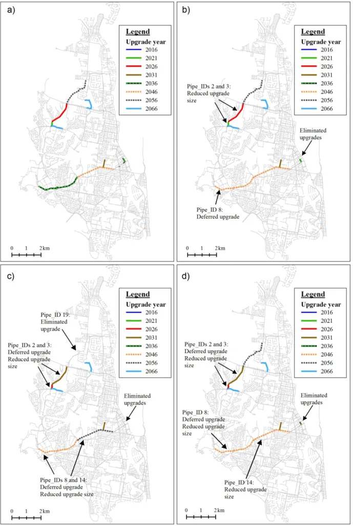
Demand curves for all of the scenarios were converted to the required units (from L/p/h to L/p/sec) and assigned to the numerous nodes in the hydraulic EPANET2 model for the city. A maximum of a three day extended-period network simulation was undertaken to fully capture the failure requirements outlined in the standards of services, and to determine the augmentation requirements for each scenario at each planning horizon. The results of the augmentation scheduling for all modelled scenarios from the model runs are illustrated in Fig. 2. The capital cost implications of the augmentation schedules for each scenario are detailed in Table 4.
As expected, the lowered peak household water demand from installing water saving measures resulted in the deferment or elimination of pipe augmentations, as well as reductions in the size of the pipe augmentations. Much of the rescheduling of the upgrades and the reduction in the pipe upgrade sizes occurred in the larger (≥500 mm) and longer water mains (i.e. trunk mains). These pipelines supply the majority of the population in both the current and future planning horizons. Hence, their scheduled augmentation arrangements are more likely to be affected by the combined reduction of peak demands from the installation of the water saving features throughout the study area. For instance, the upgrade for the pipe running easterly in the model (Pipe_ID 8), with a length of 3.1 km, was deferred by 10 years until the next planning horizon (from 2036 to 2046) for all scenarios. A 10 year deferral of upgrades (from 2046 to 2056) was also modelled for the adjoining 2.8 km pipe (Pipe_ID 14) for scenarios S3 and S4. In addition, lower peak demands reduced the sizes of both pipes from 660 mm to 525 mm for scenario S3, to 510 mm for scenario S4, and to 590 mm for scenarios S5, S6, and S7. The differences in the sizes of these two pipes are the only differences between scenarios S3 and S4, with all planned deferrals occurring at the same planning horizons. Similarly, the upgraded north easterly pipes (Pipe_IDs 2 and 3), with a total length of 2.0 km, were reduced in size from 565 mm to 500 mm for all scenarios except S2, which was sized at 510 mm. In addition, the upgrades of these two pipes were deferred by 5 years for all scenarios except S2, which had no deferrals in upgrades.
Conversely, smaller water mains serve fewer households, resulting in negligible peak demand reductions and, hence, only some augmentation deferrals are noted for these pipes. Moreover, the need to upgrade some shorter length pipes within the model, added sporadically to alleviate the high velocities and the resulting low pressures of nodes in the surrounding area, has been eliminated. The reduced peak demand from using contemporary water supplies made the pipe upgrades redundant as pipe velocities dropped and the resultant increase in node pressures reached the required range.
Fig. 2 Differences in network augmentation scheduling for scenario a) S1, b) S2, c) S3 and S4 and d) S5, S6 and S7
Table 4 Augmentation schedule and NPV costs for all scenarios S1a S2a S3a S4a S5a, b, S6 a, b, S7 a, b Pipe _ID Length (m) Diam. (mm) Upgr. year NPV Costs (AUD$c) Diam. (mm) Upgr. year NPV Costs (AUD$) Diam (mm) Upgr. year NPV Costs (AUD$) Diam (mm) Upgr. year NPV Costs (AUD$) Diam (mm) Upgr. year NPV Costs (AUD$) 1 27 200 2016 31,415 200 2016 31,415 200 2016 31,415 200 2016 31,415 200 2016 31,415 2 359 565 2021 652,337 510 2021 600,862 500 2026 517,591 500 2026 517,591 500 2026 517,591 3 1685 565 2026 2,330,055 510 2026 2,146,193 500 2031 1,848,761 500 2031 1,848,761 500 2031 1,848,761 4 12 200 2026 10,683 200 2026 10,683 200 2031 9,345 200 2031 9,345 200 2026 10,683 5 13 200 2031 10,123 200 2031 10,123 200 2046 6,775 200 2046 6,775 200 2031 10,123 6 544 200 2031 159,076 200 2031 159,076 200 2031 159,076 200 2031 159,076 200 2031 159,076 7 9 200 2036 6,130 200 2036 6,130 200 2046 4,691 200 2046 4,691 200 2036 6,130 8 3130 660 2036 5,377,823 660 2046 4,114,763 525 2046 2,388,132 510 2046 2,333,941 590 2046 2,625,450 9 114 200 2036 37,083 200 2036 37,083 - - - - - - 200 2056 21,710 10 39 200 2036 26,565 200 2036 26,565 - - - - - - 200 2036 26,565 11 61 200 2036 24,083 200 2036 24,083 - - - - - - 200 2036 24,083 12 10 200 2046 5,212 - - - - - - - - - - - - 13 55 200 2046 16,614 200 2046 16,614 200 2046 16,614 200 2046 16,614 200 2046 16,614 14 2775 660 2046 3,648,072 660 2046 3,648,072 525 2056 1,620,001 510 2056 1,583,241 590 2046 2,327,676 15 21 200 2056 8,374 200 2056 8,374 200 2056 8,374 200 2056 8,374 200 2056 8,374 16 120 200 2056 22,852 - - - - - - - - - - - - 17 131 200 2056 24,947 - - - - - - - - - - - - 18 99 200 2056 22,882 - - - - - - - - - - - - 19 2280 375 2056 914,431 375 2056 914,431 - - - - - - 375 2056 914,431 20 847 375 2066 274,857 375 2066 274,857 250 2066 120,211 200 2066 97,045 250 2066 120,211 21 32 200 2066 9,764 200 2066 9,764 200 2066 9,764 200 2066 9,764 200 2066 9,764 22 975 200 2066 111,711 200 2066 111,711 200 2066 111,711 200 2066 111,711 200 2066 111,711 23 241 200 2066 30,014 200 2066 30,014 - - - - - - - - - 24 46 200 2066 14,035 200 2066 14,035 - - - - - - - - - 25 15 200 2066 4,577 200 2066 4,577 200 2066 4,577 200 2066 4,577 200 2066 4,577 Total NPV 13,773,716 12,199,427 6,857,037 6,742,920 8,794,945
Notes: aRefer to Table 3 for description of scenarios. bS5 to S7 provided very similar reductions in mains water peak hour demand, thereby resulting in a similar network augmentation schedule. c
3.3 Financial analysis
The use of smaller sized mains and the elimination of upgrades directly reduced capital costs, while rescheduling network augmentations delayed the expenditure of capital costs when compared to the baseline scenario, thereby resulting in a lower net present cost (Table 4). Further, there was a strong correlation between peak hour demand and augmentation costs for the modelled study area. For instance, the installation of the greywater recycling (scenario S4), which produced the lowest peak demand, also resulted in the highest savings. The NPV of the pipe augmentations were reduced to AUD$6.74 million from a baseline of AUD$13.77 million; a reduction of AUD$7.03 million, which represented 51% of the original costs. The NPV of rainwater tanks use (S3) was comparable at AUD$6.86 million, with a saving of 50.2%. The lowest reductions in the peak demand was from the use of higher efficiency water appliances (S2), and produced a NPV of AUD$12.20 million, providing the lowest savings of the original costs (at 11.4%). The NPV for the scenarios incorporating the combined water saving measures (S5, S6 and S7) was AUD$8.79 million; lower than the S2 result, but higher than the S3 and S4 results, which followed a similar order to the respective peak demand. Table 5 summarises the savings and break downs of the savings for each scenario.
Table 5 NPV savings and their break downs for each scenario
Savings Break down of savings
Scenario Total NPV (AUD$a) Savings (AUD$) % of original costs
Reduced size and deferred upgr. (AUD$) % of savings Elimination of upgrades (AUD$) % of savings S1 13,773,716 - - - - S2 12,199,427 1,574,289 11.4% 1,498,396 95.2 75,893 4.8 S3 6,857,037 6,916,679 50.2% 5,794,574 83.8 1,122,104 16.2 S4 6,742,920 7,030,796 51.0% 5,908,691 84.0 1,122,104 16.0 S5, S6, S7 8,794,945 4,985,010 36.2% 4,858,829 97.6 119,942 2.4
Note: aAUD$1 = USD$0.78; June 2015.
The majority of savings was due to the deferred augmentation costs and the use of smaller sized pipes, which accounted for approximately 83.9% of the total saved costs when considering all scenarios (Table 5). Separating savings due to delayed augmentation costs and the reduced sizing costs was not possible for almost all scenarios as the deferred augmentation took place in conjunction with a reduction in pipe size for the same length of pipe, with the exception of scenario S2 (not shown in Table 5). In scenario S2, the deferred costs alone represented 80.2% of the total saved costs, while the smaller sized pipes accounted for 15% of the savings with the eliminated upgrades making up the remaining 4.8% of the saved costs.
Although the bulk of the savings came from the reduced augmented costs of the larger mains with Pipe_IDs 2, 3, 8, and 14 (Table 4), especially the latter two pipes, the results clearly demonstrate the monetary benefits of reducing peak demand within the water supply network. Also, while scenario S2 may suggest that the majority of the capital savings would occur from the deferred costs, the contributing factors for the network upgrades may differ due to the differential costs in a much smaller sized water supply network, or as a result of the differing urban expansion forms within the same area (Farmani and Butler, 2014; Marques et al., 2015). For example, the reduced pipe sizes, rather than deferred costs, may contribute towards most of the
savings. In any case, the results have demonstrated the potential for water utilities to extract considerable financial savings from the installation of mains water saving measures; even the application of water efficient appliances provided measureable capital savings.
4 Discussion
4.1 Influence of timing of peak demand on network augmentations
The timing of the peak demand for the various water saving measures is noted to affect the scheduling of network augmentations. It should be noted that since this study considered infill development over time, the majority of the households in all planning horizons consisted of baseline (Profile A) housing stock from the base planning horizon (i.e. 2011) plus 40% of the new stock, which did not include alternative water sources or high efficiency appliances. The timing of the baseline profile’s peak demand, which occurred at normal peak hours (8 am and 6 pm), were found to influence the upgrade plans of the water supply network, mainly for the trunk mains. The modelled peak flows for the rainwater tanks and greywater reuse occurred at off-peak hours; with demand at normal off-peak hours for these alternative water sources lower than their actual peak flows (refer to Fig. 1). This resulted in the upgrading of the larger mains for scenarios incorporating alternative water supplies to be influenced by this lower peak hour demand, rather than by the actual peak flow. As the peak hour demand for both alternative water sources are similar, the scheduling of their augmentations would also be comparable. For this reason, the hydraulic model run findings for scenario S3 resulted in similar levels of network upgrades to scenario S4. Furthermore, there were no differences in the augmentation scheduling observed for the scenarios comprising a combination of water saving measures (S5, S6, and S7). It is noted that only the upgrades of larger mains appear to be affected by the normal peak hour demand. For smaller pipes supplying to households in an area fitted mainly with alternative water supplies, the peak flows would still be the driving factor in the sizing of the pipes and, hence, their augmentations.
4.2 Implications of reduced peak demand on water infrastructure
This study has empirically demonstrated that a strategy for implementing mains water saving measures across a city can reduce water distribution network peak demand, which in turn leads to deferrals or the elimination of planned pipe network upgrades, ultimately reducing capital cost schedules by around half. Developers might be persuaded to install the highest efficiency appliances or rain/recycling water systems on their new projects if a rebate or infrastructure charge reduction was provided to them; a proposal on this is provided in the next section.
In addition to the capital savings shown herein, the installation of water saving measures would also reduce the utilities future operating costs with pump stations running more efficiently (i.e. less electricity to pump water during peak periods) and through the treatment and transport of lower volumes of water (Malinowski et al., 2015). For water utilities in areas where peak energy tariffs are higher than the rest of the day, the on-peak reduction of water demand could potentially reduce water systems on-peak electrical demands, and provide additional financial benefits (House and House, 2012). Furthermore, the asset life could be extended, and
pipe failures minimised, as a result of the reduced flow in the pipeline, leading to less distribution leakage and, hence, reduced maintenance costs.
4.3 Choice of diversified water supply scheme within a water supply zone
Fig. 2 illustrated similar levels of augmentations for rainwater tanks and greywater recycling, while Table 4 and Table 5 highlighted their similarities in incurred capital costs and savings. In this regard, it is worthwhile determining and comparing the financial feasibility of both of these sources of alternative water supplies. The economic viability of greywater against rainwater reuse depends on the former’s level of treatment. Greywater treated at lower levels would potentially provide shorter payback periods compared to rainwater tanks (Ghisi and Ferreira, 2007; Ghisi and Oliveira, 2007). However, in urban areas, where space is limited, higher levels of greywater treatment are required and makes their reuse more expensive (Li et al., 2010; Mourad et al., 2011). Nevertheless, both greywater and rainwater used on a larger scale are acknowledged to be more economically feasible than if used in single-residential households (Friedler and Hadari, 2006; Gurung and Sharma, 2014; Mourad et al., 2011).
With greywater reuse proving to be a more expensive option than rainwater tanks in urban areas, and as infrastructure capital savings for both alternative water sources are the same; it appears to be more economically viable to install rainwater tanks due to a potentially higher net balance (NPV of infrastructure upgrade savings minus NPV of water saving measures). Indeed, the cheapest option is to install only higher efficiency water appliances, although it also delivers the least capital savings (Table 4). Consequently, a cost benefit analysis is required to determine if these water saving measures would actually provide net positive benefits. Water utilities can then determine the relevant incentives for developers to balance the cost of installing these measures, especially in large-scale infill developments. For instance, land developers are usually charged a water infrastructure cost by water utilities to recoup the cost for providing water supply to a city. However, there could be an opportunity for water utilities to implement an alternative water infrastructure charge policy for land developers who install water efficiency or source substitution measures, with the saved capital expenditure being shared amongst the developers through reduced infrastructure charges (Gurung et al., 2015; Sharma et al., 2012).
Such a strategy would present an ideal situation as utilities, developers, and consumers benefit from a more efficient water supply system. This win-win, top-down, and bottom-up planning and costing of utility infrastructure is undoubtedly needed in the future. The evidence presented herein provides another welcome dividend (i.e. deferment of pipe network distribution infrastructure upgrades) for the water efficiency agenda, and goes beyond the already demonstrated benefits of using efficiency and potable source substitution measures for extending supply reliability and deferring the requirement for bulk water supply infrastructure such as desalination plants or dams (e.g. Sahin et al., 2015).
4.4 Smart water meters for assisting in network augmentations
Given that existing traditional building stock will be the majority in brownfield locations and will still be the major consumers of water, utilities should try to reduce the peak hour demand from these customers. Apart
from fitting current households with the highest rated water appliances, installing smart water meters provides a means of achieving this target by presenting an excellent opportunity for water utilities to implement time of use tariffs (TOUT). TOUT could either be implemented to impose penalty charges for exceeding a consumption threshold over a specific period of the day (Cole and Stewart, 2013) or to provide monthly incentives for lowering peak hour consumption (House and House, 2012). The implementation of TOUT could be further supported with the development of a real time web-portal visualisation tool which would assist and inform customers on where exactly their water is being consumed (e.g. Stewart et al., 2010). Such incentives and tools would provide added motivation for consumers to spread their water use throughout the day, enabling innovative social marketing strategies, which would promote the shifting of individual end-use peak demand to off-peak times of the day (House and House, 2012; Beal et al., 2016). The incentive based approach would encourage a higher uptake of such strategies, in the absence of which, the attitudes, beliefs and habits of customers would be a key factor in influencing the uptake of such behavioural strategies (Beal et al., 2016). These strategies, with the assistance of smart water meters, would enable consumers to proactively reduce their normal peak hour demand, and consequently enable water utilities to take advantage of the network capital savings.
In this study, smart water meter data were used as the base for modelling water demand profiles for various water saving scenarios, thus demonstrating smart water meters’ capability to be used as an updated water demand forecasting tool. This outcome can be further advanced through investigating current trends in water consumption from real-time records of smart water meter data stored in a central location. If actively utilised, it would allow for a continual adaptation of water demands and usage patterns. Additionally, such “live” data can be loaded instantaneously into water supply models allowing for a bottom-up just-in-time modelling approach to be adopted, enabling a more accurate representation of the current status of the water supply network. Essentially, smart water meter-derived forecasted consumption trends, demand values, and even the actual data itself, can be applied to hydraulic models for different planning horizons, to more accurately predict the planning of future network upgrades. However, at present, their installation requires a high upfront cost for a citywide rollout, along with considerable work on utility change management, data collection protocols and end-use classifications (Beal and Flynn, 2015). Nevertheless, this situation is fast changing with greater production of smart metering technology as well as the rapidly developing hydroinformatic applications being realised (e.g. Britton et al. 2013; Fontdecaba et al., 2013; Nguyen et al., 2014).
5 Conclusion
The study demonstrated the extent to which diversified water supply schemes can provide monetary savings in the water supply network through reduced household peak water demand; with NPV capital savings of up to 51% determined in this study. Specifically, the study empirically determined that household peak water demand had a strong correlation with costly pipe network upgrades, and that these peaks could be substantially reduced through efficiency and source substitution strategies. Modelled water demand profiles of diversified water supply schemes using intelligently gathered and analysed smart water meter data
demonstrated that outdated approaches to water demand modelling, often employed by water service providers and their consultants, is not sufficiently sophisticated in an era where water supply options have become more diversified and the associated water demand patterns more complex to estimate.
The results of the study provides added motivation for water utilities to continually promote the use of water saving measures by providing incentives (e.g. alternative water charges) for the implementation of such schemes, so that capital cost savings can be achieved. Essentially, the influence of water saving schemes on the water supply network should not be ignored and must be accurately account for in contemporary modelling practices. In this case, smart water meters offer water utilities a range of benefits, such as, up-to-date consumption data and ability to implement further peak demand reducing solutions (e.g. TOUT), making them efficient tools in the operation, management and planning of water infrastructure.
While beyond the scope of this current study, future work would undoubtedly reveal further related savings in water distribution network operational costs (e.g. pumping). Moreover, future work should consider how smart meter enabled TOUT arrangements, customer feedback applications, and sophisticated just-in-time network modelling would all contribute to the extraction of further efficiency dividends in the water distribution network. Furthermore, a similar study to that herein but focused on the under-researched commercial and industrial sectors is of future research priority, in order to understand the capital savings contributions of all segments of the water sector.
Acknowledgements
The authors are grateful to the City of Gold Coast for their financial and in-kind support, as well as the participants of the various smart metering and water end-uses studies.
References
ABS (Australian Bureau of Statistics) (2014). 6427.0 - Producer Price Indexes, Australia, Dec 2014, Available at: http://www.abs.gov.au/ausstats/[email protected]/mf/6427.0 (accessed February 2015).
Alcocer-Yamanaka, V., Tzatchkov, V., and Arreguin-Cortes, F. (2012). “Modeling of drinking water distribution networks using stochastic demand.” Water Resources Management, 26, 1779-1792. Beal, C. D., and Stewart, R. A. (2011). “South East Queensland residential end-use study: Final report.”
Urban Water Security Research Alliance Technical Report No. 47, Queensland Government, Australia.
Beal, C. D., and Stewart, R. A. (2014). “Identifying residential water end-uses underpinning peak day and peak hour demand.” Journal of Water Resources Planning and Management, 140(7), 04014008. Beal, C. D., and Flynn J. (2015). “Toward the digital water age: Case studies of Australian water utility
Beal, C. D., Gurung, T. R., and Stewart R. A. (2016). “Demand-side management for supply-side efficiency: an exploration of tailored strategies for reducing peak residential water demand.” Sustainable Production and Consumption, 26(6), 1-11.
Blokker, E. J. M., Vreeburg, J. H. G., van Dijk, J. C. (2010). “Simulating residential water demand with a stochastic end-use model.” Journal of Water Resources Planning Management, 136(1), 19-26
Britton, T. C., Stewart, R. A., O’Halloran, K. R. (2013). “Smart metering: enabler for rapid and effective post meter leakage identification and water loss management.” Journal of Cleaner Production. 54, 166-176
Carragher, B. J., Stewart, R. A., and Beal, C. D. (2012). “Quantifying the influence of residential water appliance efficiency on average day diurnal demand patterns at an end use level: A precursor to optimised water service infrastructure planning.” Resources, Conservation and Recycling, 62, 81-90. Chrisotva-Boal, D., Eden, R. E., and McFarlane, S., (1996). “An investigation into greywater reuse for urban
residential properties.” Desalination, 106, 392-397
Cole, G., and Stewart, R. A. (2013). “Smart meter enabled disaggregation of urban peak water demand: precursor to effective urban water planning.” Urban Water Journal, 10(3), 174-194.
DHPW (Department of Housing and Public Works). (2013). “MP 4.1 – Sustainable Buildings.” Queensland
Government, February 2013. Available at:
http://www.hpw.qld.gov.au/SiteCollectionDocuments/QDCMP4.1SustainableBuildingsCurrent.pdf
(accessed February 2015).
DIP (Department of Infrastructure and Planning). (2008). “Greywater guidelines for plumbers, A guide to the use of greywater in Queensland”, Queensland Government, August 2008. Available at:
http://www.hpw.qld.gov.au/SiteCollectionDocuments/greywater-guidelines-plumbers.pdf (accessed February 2015).
DTF (Department of Treasury and Finance). (2003). “Use of discount rates in the partnerships Victoria process.” Partnerships Victoria-Technical note-July 2003.
Farmani, R., and Butler, D. (2014). “Implication of urban form on water distribution systems performance.”
Water Resources Management, 28(1), 83-97.
Fontdecaba, S., Sánchez-Espigares, J. A., Marco-Almagro, L., Tort-Martorell, X., Cabrespina, F., and Zubelzu, J. (2013). “An approach to disaggregating total household water consumption into major end-uses.” Water Resources Management, 27(7), 2155-2177.
Friedler, E., and Hadari, M. (2006). “Economic feasibility of on-site greywater reuse in multi-storey buildings.” Desalination, 190(1-3), 221-234.
GCW (2009) Gold Coast Water (2009-A), “Desired Standards of Service Review 2008”, GHD Final Report Rev 3, October 2009
Ghisi, E., and Ferreira, D. F. (2007). “Potential for potable water savings by using rainwater and greywater in a multi-storey residential building in southern Brazil.” Building and Environment, 42(7), 2512-2522.
Ghisi, E., and de Oliveira, S. M. (2007). “Potential for potable water savings by combining the use of rainwater and greywater in houses in southern Brazil.” Building and Environment, 42(4), 1731-1742. Gil, H. A., and Joos, G. (2006). “On the quantification of the network capacity deferral value of distributed
generation.” IEEE Transactions on Power Systems, 21(4), 1592-1599.
Gurung, T. R., and Sharma, A. (2014). “Communal rainwater tank systems design and economies of scale.”
Journal of Cleaner Production. 67, 26-36.
Gurung, T. R., Stewart, R. A., Sharma, A. K., and Beal, C. D. (2014). “Smart meters for enhanced water supply network modelling and infrastructure planning.” Resources, Conservation and Recycling, 90, 34-50.
Gurung, T. R., Stewart, R. A., Beal, C. D., and Sharma, A. K. (2015). “Smart meter enabled water end-use demand data: platform for the enhanced infrastructure planning of contemporary urban water supply networks.” Journal of Cleaner Production, 87, 642-654.
Haque, M., Hagare. D, Rahman, A. and Kibria, G. (2014). “Quantification of water savings due to drought restrictions in water demand forecasting models.” Journal of Water Resources Planning and Management, 140(11), 04014035.
House, L. W., and House, J. D. (2012). “Shifting the timing of customer water consumption.” Journal-American Water Works Association, 104(2), E82-E92.
Li, Z., Boyle, F., and Reynolds, A. (2010). “Rainwater harvesting and greywater treatment systems for domestic application in Ireland.” Desalination, 260(1-3), 1-8.
Lucas, S. A., Coombes, P. J., and Sharma, A. K. (2010). “The impact of diurnal water use patterns, demand management and rainwater tanks on water supply network design.” Water Science & Technology: Water Supply-WSTWS, 10(1), 69-80.
Malinowski, P., Stillwell, A., Wu, J., and Schwarz, P. (2015). “Energy-water nexus: Potential energy savings and implications for sustainable integrated water management in urban areas from rainwater harvesting and gray-water reuse.” Journal of Water Resources Planning and Management, doi: 10.1061/(ASCE)WR.1943-5452.0000528, A4015003.
Marques, J., Cunha, M., and Savić, D. (2015). “Using Real Options in the Optimal Design of Water Distribution Networks.” Journal of Water Resources Planning and Management, 141(2), 04014052. Mourad, K. A., Berndtsson, J. C., and Berndtsson, R. (2011). “Potential fresh water saving using greywater
Nguyen, K. A., Stewart, R. A., and Zhang, H., (2014). “An autonomous and intelligent expert system for residential water end-use classification.” Expert Systems with Applications. 41(2), 342-356.
Piccolo, A., and Siano, P. (2009). “Evaluating the impact of network investment deferral on distributed generation expansion.” IEEE Transactions on Power Systems, 24(3), 1559-1567.
Rathnayaka, K., Malano, H., Maheepala, S., Nawarathna, B., George, B., and Arora, M. (2011). “Review of residential urban water end-use modelling.” 19th International Congress on Modelling and Simulation, Perth, Australia, December 12–16.
Rossman, L. A. (2000). “EPANET2 Users Manual.” US Environmental Protection Agency. Cincinnati, OH Sahin, O., Stewart, R. A., and Porter, G. (2015). “Water security through scarcity pricing and reverse
osmosis: a system dynamics approach.” Journal of Cleaner Production, 88, 160-171.
Savic, D. A. and Walters, G. A. (1997). “Genetic algorithms for least-cost design of water distribution networks.” Journal of Water Resources Planning and Management, 123, 67-77.
SEQ Code (South East Queensland Code). (2013). “South East Queensland water supply and sewerage
design and construction code.” Queensland. http://www.seqcode.com.au/storage/2013-07-01%20-%20SEQ%20WSS%20DC%20Code%20Design%20Criteria.pdf (accessed December 2014).
Sharma, A. K., Cook, S., Tjandraatmadja, G. and Gregory, A. (2012). “Impediments and constraints in the uptake of water sensitive urban design measures in greenfield and infill developments.” Water Science and Technology, 65(2), 340-352.
Stewart, R. A., Willis R. M., Giurco, D., Panuwatwanich, K., and Capati, B. (2010). “Web-based knowledge management system: linking smart metering to the future of urban water planning.” Australian Planner, 47(2), 66-74.
Swamee, P. K., and Sharma, A. K. (1990). “Reorganisation water distribution system.” Journal of Environmental Engineering, 116(3), 588-600.
Swamee, P. K., and Sharma, A. K. (2008). Design of Water Supply Pipe Networks, John Wiley and Sons, New Jersey, USA.
Umapathi, S., Chong, M. N., and Sharma, A. K. (2013). “Evaluation of plumbed rainwater tanks in households for sustainable water resource management: a real-time monitoring study.” Journal of Cleaner Production, 42, 204-214.
Walski, T. M., Chase, D. V., Savic, D. A., Grayman, W., Beckwith, S., and Koelle, E. (2003). Advanced Water Distribution Modeling and Management. Haestad Methods, Inc. Waterbury, CT.
Willis, R. M., Stewart, R. A., Williams, P. R., Hacker, C. H., Emmonds, S. C., and Capati, G. (2011). “Residential potable and recycled water end uses in a dual reticulated supply system.” Desalination, 272(1-3), 201-211.
Willis, R. M., Stewart, R. A., Giurco, D. P., Talebpour, M. R., and Mousavinejad, A. (2013). “End use water consumption in households: impact of socio-demographic factors and efficient devices.” Journal of Cleaner Production, 60, 107-115.
View publication stats View publication stats