Mapping directed influence over the brain using Granger causality
and fMRI
Alard Roebroeck,* Elia Formisano, and Rainer Goebel
Department of Cognitive Neuroscience, Faculty of Psychology, University of Maastricht, the Netherlands Received 4 August 2004; revised 15 October 2004; accepted 1 November 2004
Available online 12 January 2005
We propose Granger causality mapping (GCM) as an approach to explore directed influences between neuronal populations (effective connectivity) in fMRI data. The method does not rely on a priori specification of a model that contains pre-selected regions and connections between them. This distinguishes it from other fMRI effective connectivity approaches that aim at testing or contrasting specific hypotheses about neuronal interactions. Instead, GCM relies on the concept of Granger causality to define the existence and direction of influence from information in the data. Temporal precedence information is exploited to compute Granger causality maps that identify voxels that are sources or targets of directed influence for any selected region-of-interest. We investigated the method by simulations and by application to fMRI data of a complex visuomotor task. The presented exploratory approach of mapping influences between a region of interest and the rest of the brain can form a useful complement to existing models of effective connectivity.
D2004 Elsevier Inc. All rights reserved.
Keywords:Effective connectivity; fMRI; Granger causality; Autoregressive models
Introduction
Functional brain imaging has contributed substantial insights into the neural correlates of human information processing and cognitive operations. Most research with positron emission tomography (PET) and functional magnetic resonance imaging (fMRI) has focused on relevant information about where information is processed in the human brain. To improve our understanding of how the brain processes information, more knowledge about the interactions of activated brain areas, that is,
functional integration (Friston, 2002) is needed. The investigation of functional integration with PET and fMRI data has been pioneered by several researchers (Friston et al., 1993a,b; Horwitz, 1990; Horwitz et al., 1992; McIntosh et al., 1993). Their work has lead to a rapid increase in investigations of functional integration with PET and fMRI for various cognitive or sensorimotor tasks. A model-free approach to study functional integration is to investigate the correlation between measured time courses of different brain areas, which has been referred to as functional connectivity (Friston et al., 1993b). However, func-tional connectivity is ambiguous with respect to underlying directed interactions that generated the observed correlations. Effective connectivity, defined as the influence one neuronal system exerts over another (Friston, 1994; Friston et al., 1993a), attempts to resolve this ambiguity by defining explicit statistical models of directed neuronal interactions. Recently, significant methodological advances in effective connectivity modeling have been made, such as the application to neuroimaging data of covariance structural equation modeling (Buchel and Friston,
1997; McIntosh and Gonzalez-Lima, 1994), nonlinear system
identification techniques (Friston and Buchel, 2000), and Baye-sian estimation of deterministic state-space models (Friston et al., 2003). However, effective connectivity methods proposed so far all require preselection of the interacting regions and assumptions about the existence and direction of influence between any two regions. These pre-specified models are useful in specifying and testing specific hypothesis concerning interactions between brain systems. However, an implicit problem in this type of approach is that misspecification of the models (e.g., by omission of an area that mediates or initiates interactions) can lead to erroneous conclusions.
Here, we present a framework to map effective connectivity over the brain using vector autoregressive (VAR) modeling of fMRI time series in the context of Granger causality (Granger, 1969, 1980). Assuming thatx[n] andy[n] are the measured time courses of two brain regions (or voxels), Granger causality quantifies the usefulness of unique information in one of the time series in predicting values of the other. Specifically, if incorporat-ing past values ofx improves the prediction of the current value ofy, we say thatx Granger causesy. Thus, temporal precedence 1053-8119/$ - see front matterD2004 Elsevier Inc. All rights reserved.
doi:10.1016/j.neuroimage.2004.11.017
* Corresponding author. Capaciteitsgroep Neurocognitie, Faculteit der Psychologie, Postbus 616, 6200 MD Maastricht, the Netherlands. Fax: +31 43 3884125.
E-mail address: [email protected] (A. Roebroeck). Available online on ScienceDirect (www.sciencedirect.com.)
is used to identify the direction of causality from information in the data. In our framework, time-resolved fMRI measurements provide topographical as well as temporal information about the brain areas subserving a cognitive task. Temporal precedence information is exploited to compute Granger causality maps (GCMs) that identify voxels that are sources or targets of directed influence for any selected region-of-interest. Thus, the method is exploratory in nature and does not require the specification of a directed graph model.
Granger causality analysis has been previously applied to electrophysiological animal data, specifically Local Field Poten-tials (LFPs) to detect influences at the neuronal population level (Baccala and Sameshima, 2001; Bernasconi and Konig, 1999; Bernasconi et al., 2000; Brovelli et al., 2004; Freiwald et al., 1999). More recently, Granger causality and related frequency domain measures have also been applied to human EEG data (Hesse et al., 2003; Kaminski et al., 2001). Furthermore, multivariate autoregressive models have recently also been applied to human fMRI data to model effective connectivity between preselected regions based on temporal order (Harrison et al., 2003), thus making implicit use of the concept of Granger causality. We have previously reported initial investigations of the application of Granger causality to fMRI data (Goebel et al., 2003, 2004). However, there are two potential obstacles for the successful application of Granger causality to fMRI signals. First, fMRI only provides indirect access to the neuronal responses and information on dynamic interactions between neuronal popula-tions may be irremediably lost or distorted by hemodynamic blurring of the neuronal responses. Second, the applicability of Granger causality may also be limited because of the relatively low temporal resolution of data acquisition techniques conven-tionally employed. In order to investigate the constraints posed by hemodynamics and temporal sampling, we performed a series of simulation studies. Our simulations show that it is possible to recover directed neuronal influences from the fMRI signal if short volume repetition times (TRs) are used. After describing the simulation studies, we describe an application of Granger causality mapping to fMRI data for a dynamic visuomotor mapping task. To assess significance of the obtained GCMs, we developed thresholding methods based on bootstrapping techni-ques (Efron and Tibshirani, 1993) and the control of the false discovery rate for voxelwise tests (Genovese et al., 2002). The method identified directed interactions between inferotemporal, parietal, and premotor areas that underlie the performance of a complex visuomotor task.
Theory
The discrete zero-mean vector time-series x[n] = (x1[n], . . .,
xM[n])Tcan be modeled as a vector autoregressive (VAR) process
of orderp(e.g.,Kay, 1988):
x½ ¼ n X p
i¼1
A½ ix½ni þu½ n
where u[n] is (multivariate) white noise. The matrices A[i] are called the autoregression (AR) coefficients because they regress
x[n] onto its own past. The VAR model can be thought of as a linear prediction model that predicts the current value ofx[n] based on a linear combination of the most recent past p values. Consequently, the current value of a componentxi[n] is predicted
based on a linear combination of its own past values and the past values of the other components. This shows the value of the VAR model in quantifying Granger causality between (groups of) components.
Granger causality uses temporal precedence to identify the direction of causality from information in the data. Thus, given two time series x[n] and y[n], we can independently identify both influence fromx toy, and influence in the reverse direction with suitable models.Geweke (1982)has proposed a measure of linear dependenceFx,ybetweenx[n] andy[n] which implements Granger
causality in terms of vector autoregressive models (see Appendix A for details).Fx,yis the sum of three components:
Fx;y¼FxYyþFyYxþFxSy
the four measures take their values in the interval [0,l), that is, they are by construction nonnegative. Fx,y is a measure of the
total linear dependence between the seriesx andy. If nothing of the value at a given instant of one can be explained by a linear model containing all the values (past, present, and future) of the other, Fx,y will evaluate to zero. FxYy is a measure of linear
directed influence from x to y. If past values of x improve the prediction of the current value of y, then FxYy N 0. A similar interpretation holds, of course, for FyYx. Thus, the two directed
components,FxYy andFyYx, use the arrow of time to decide on
the direction of influence. However, the total linear dependence between x and y does not often consist fully of these directed components. Much of the total linear dependence can be contained in the undirected instantaneous influenceFxdy between
them. Essentially, Fxdy quantifies the improvement in the
prediction of the current value of x (or y) by including the current value ofy(orx) in a linear model already containing the past values of x and y. From this symmetry it can be seen that Fxdy indeed contains no directional information at all. It
represents residual correlations in the data that cannot be assigned to causally directed influence based on the information in the data. In practice, nonzero values of Fxdy can be caused by
directed influence betweenxandy at a finer time-scale than that at which x and y are observed (Granger, 1969, 1980). We investigated the usefulness and validity of these measures in investigating effective connectivity in fMRI data, both by simulations and by application to real fMRI data.
Simulations
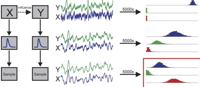
Based on the observed high correlation between Local Field Potentials (LFPs) and the Blood Oxygenation Level Dependent (BOLD) response (Logothetis et al., 2001), we can approximate fMRI signals with a low-pass filtered and sub-sampled version of LFPs. Previous invasive electrophysiological studies have shown that statistical techniques based on VAR-modeling and Granger causality are capable of detecting directed interactions between neuronal populations as reflected in the dynamic structure of LFP signals (Bernasconi and Konig, 1999; Bernasconi et al., 2000; Brovelli et al., 2004; Freiwald et al., 1999). We used simulations to investigate whether and to what extent this capability is preserved with fMRI measurements. We assumed neuronal interactions to occur at the level of LFP signals and quantified the effects of 1) hemodynamics (i.e., filtering) and 2) fMRI image collection (i.e., temporal sampling of BOLD responses) on computed Granger causality measures (seeFig. 1).
The signals x[n] and y[n] of two interacting neuronal populations X and Y were generated as a realization of a bi-dimensional first-order VAR process with:
A½ ¼1 0:9 0 I 0:9 ;¼ 1 0 0 1
this model has the benefit of being simple while still allowing achievement of the desired dynamic characteristics. The model was specified to have the following properties: First, it embodies an influence fromX(its first channel, the influencing brain region) to Y (its second channel, the brain region being influenced) of a predetermined strengthI (ranging from 0.0, no influence, to 0.5, strong influence). Second, by construction, there is no influence in the reverse direction from Y to X, rendering the modeled interaction strictly unidirectional. Third, the influence from X to Ywas manipulated to have an additional delayD(ranging from 0 to 100 ms) representing the time that passes before the population dynamics in X has an influence on Y’s dynamics. Fourth, instantaneous dependence betweenX’s signalx[n] andY’s signal
y[n] was also absent by construction (i.e., the off-diagonal terms in are zero). Fifth, the auto-regressive coefficients on the diagonal (i.e., connectingx[n] andy[n] to their own respective pasts) were set such that all of their spectral power is contained in the lower frequency ranges. Thus, the influence X exerts on Y was constructed to take place in the lower frequency ranges. This is in line with the expectation that high-frequency dependencies between x[n] and y[n] are not detectable after passing through hemodynamics (essentially a low-pass filter) and being down-sampled in the data acquisition. This would in turn transfer to the interpretation that the directed influences detected in real fMRI data would depend on low-frequency signal fluctuations, perhaps caused by the experimental design.
The time-step of the simulation was taken to be 10 ms. In every simulation, the model was simulated for 10,000 time-steps (100 s), where additionally an initial 2000 + D time-steps were simulated and later discarded to allow the system to enter a steady state, to introduce the delay D and to avoid boundary effects in subsequent filtering. After simulation and introduction of addi-tional delay, the channels were individually filtered by convolu-tion with a linear model of the Hemodynamic Response Funcconvolu-tion (HRF) based on a gamma function (Boynton et al., 1996). The tau parameter in this model, controlling the width of the HRF, was set to 0.5, corresponding to short (0.5 s) stimulus durations (Liu and Gao, 2000), relevant for fast event-related designs. After individually normalizing the channels to zero mean and unit variance, 20% of white Gaussian noise was added, representing physiological noise in the BOLD response. Subsequently, these simulated BOLD response signals were sampled every S time-steps to simulate signal acquisition by the scanner with a whole volume TR of S/100 s. After renormalizing the signals, another 20% of white Gaussian noise was added to represent measure-ment error and noise in the acquisition. Note, that noise enters the simulated system at three independent points. First, in the form of the innovation u[n] that drives the dynamics of the VAR model that generates the simulated LFPs. Second, noise is added at the level of the hemodynamics, mimicking imperfections in the transfer of neuronal signals to hemodynamic signals. Third, noise is added at the level of sampling by the MR-scanner, simulating additive instrumental noise. The resulting signals were used to compute influence measuresFxYy,FyYx, andFxdy. The order p
of the estimated autoregressive models was set to that which minimized the Schwartz Criterion (SC), an order selection criterion, designed to trade-off the reduction in error-variance against the increase in the number of parameters (Luetkepohl, 1991).
Fig. 1. A schematic illustration of the procedure to generate simulated time series (in the leftmost column), examples of the generated series at various stages (in the middle column), and of resulting distributions of computed influence values for 5000 simulations (in the rightmost column). The top row depicts the generation of simulated local field potential (LFP) signals ofXandYat high temporal resolution. The simulation model implements a temporally directed influence fromXtoY. The middle row represents the filtering of the LFP signals through a canonical hemodynamic response model to obtain simulated blood oxygenation level dependent (BOLD) signals. The bottom row shows how a temporal down-sampling of the BOLD signals then gives the simulated fMRI signal. Influence measuresFxYy,FyYx, andFxdycan be computed from the generated time series at all three stages. If the simulation is repeated many times
(e.g., 5000), distributions of the influence measures can be obtained. These are shown in the rightmost column, where the distributions ofFxYyvalues is shown
in blue,FyYxdistributions are shown in green andFxdydistributions are shown in red. The set of distributions for the simulated fMRI signal (in the red box) is
Simulations were performed for systematic combinations of the levels of crucial parameters in the model: the strength of influence (I= {0.0, 0.1, 0.2, 0.3, 0.4, 0.5}), the delay of influence (D= {0, 1, 2, 3, 4, 5, 6, 7, 8, 9, 10}), and the temporal sampling (S= {10, 20, 30, 40, 50, 60, 70, 80, 90, 100}). For each of the 660 possible combinations of these parameters, a set of 5000 simulations was performed and influence measures FxYy, FyYx, and Fxdy were
computed on the simulated sampled signals. Inference was performed in the context of the bootstrap (Efron and Tibshirani, 1993), which is based on empirically obtained null distributions (See Appendix B for details). Significance thresholds can be obtained both within the classical framework, controlling for Type I error (quantified by the proportion of false positives within all tests), and with methods controlling for the false discovery rate (FDR, the expected proportion of false positives within all tests with a positive result) and which are more appropriate in the context of mapping effects over an imaging volume (Genovese et al., 2002). An empirical null distribution for the simulations was formed by computing the influence measures on pairs of signals
x[n] and y[n] from different simulations in the same set. Any dependence between two channels from different realizations of
the model can only exist purely by chance and thus characterize the null hypothesis of no influence.
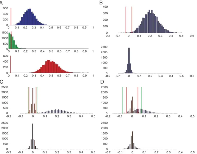
Fig. 2A shows the distributions of values obtained for FxYy,
FyYx, and Fxdy in an exemplary set of simulations. Two
observations can be made from these distributions. First, the values found forFxYyare, on average larger than those found for
FyYx, reflecting the true influences present at the LFP level.
Second, the values found for Fxdy are markedly different from
zero, pointing to instantaneous influence between X and Y not actually present at the LFP level. This finding is not surprising because we are applying Granger causality to time-series sampled at a courser interval than that at which interactions take place (Granger, 1969, 1980). The instantaneous influence term essen-tially quantifies partial correlation (functional connectivity) that cannot be assigned to influence in a certain direction purely from temporal information in the data. As a general pattern over all simulations, the levels of instantaneous influence found were large and increased with increasing sample interval. Since our interest is mainly in directed influences, the finding of instantaneous influences need not be a conceptual difficulty. When found in absence of additional directed influence, it merely points to the
Fig. 2. Distributions of influence measures resulting from 5000 simulations. In (A) histograms are shown forFxYyvalues in blue in the upper panel, forFyYx
values in green in the middle panel, and forFxdyvalues in red in the lower panel for 5000 simulations withI= 0.3,D= 50 ms, andS= 0.5 s. The
influence-difference terms for the same simulation set are shown in the upper panel of (B), along with the associated empirical null distribution in the lower panel. The same distribution of difference terms is shown again in blue in the upper panel of (C) along with its null distribution in blue in the lower panel. Superimposed in red is the difference distribution of 5000 simulations withI= 0.0 (andDandSas before) with its associated null distribution in red in the lower panel. In (D), the same distributions are shown withS= 100 (1.0 s). Vertical red lines indicate classical significance thresholds ata= 0.05, and vertical green lines indicate FDR-based thresholds atq= 0.05, based on the empirical null distributions. Thresholds in C and D were computed from the joined set of values forI= 0.3 and I= 0.0.
necessity to incorporate further assumptions (such as those in structural equation models (McIntosh and Gonzalez-Lima, 1994) or dynamic causal models (Friston et al., 2003)) when inference on effective connectivity is needed.
Thus, we turn to inference on FxYy and FyYx. Classical
significance thresholds for a = 0.05 are shown in Fig. 2A. All FxYy values are above threshold, suggesting that there is good
sensitivity in detecting influence from X to Y even after interference of hemodynamics and temporal down-sampling. However, a much larger proportion of FyYx values are above
threshold than the nominal 0.05, showing that, in the context of fMRI data, inferences on directed influences based on the simple terms introduced above may be biased. Conceptually, the problem of unidirectional influence turning into bi-directional interaction (Wei, 1990) is due to the unavoidable loss of dynamic stochastic information in both channels of the system arising from low-pass filtering and down-sampling of the signals. In other words, some part of the variance inx[n] that could previously be explained byX’s past, is now explained byY’s past, since the relevant information in X’s past is lost. This leads to an inflation of theFyYxmeasure.
A possible solution to this inference problem, suggested by the observed distributions ofFxYy and FyYx is to perform inference
not on their individual values, but on their difference (FxYy
FyYx). Positive values of this influence difference term would
point to influence from X to Y, whereas negative values would indicate influence in the reverse direction. The distribution of (FxYyFyYx) for the same set of simulations as before is shown
inFig. 2B, together with its empirical null distribution. It can be seen from the significance thresholds for a two-sided test for non-zero values that inference on the difference term behaves very well. A very large proportion of values (N0.99) is significantly positive, again indicating very good sensitivity. Moreover, only a very small proportion (much smaller than 0.05) of values is significantly negative, indicating good specificity. The observation of a smaller than the nominal proportion of false positives was in fact repeated over the full range of values ofI,D, andS. It should be noted that the regained robustness in inference on unidirectional influences comes at the cost of a lack of sensitivity to true bi-directional interactions (see Discussion).
Because the main goal of our approach is to map directed influences over the whole brain, sensitivity and specificity were investigated further within the framework of FDR-based hypoth-esis testing (see Appendix B). In this testing framework, methods are employed that control the FDR (the expected proportion of false positives within all tests with a positive result) even over a large number of tests, thus presenting an approach to the multiple comparison problem (Genovese et al., 2002). To evaluate perform-ance of FDR-based inference on the influence difference terms, FDR-based thresholds were computed for sets of 10,000 simu-lations ofx[n] andy[n]. In half of the cases there existed influence fromXto Y (with given strengthI and delayD), whereas in the other half there was no influence between the simulated signals (i.e.,I= 0.0). This forms a more realistic inference situation where cases of true influence must be detected within a larger set (e.g., an imaging volume) of dynamically varying signals. To quantify performance of the inference on the influence-difference terms, the empirical power (as a measure of sensitivity) was computed, for a given threshold, as the proportion of true positives within all tests, that is, the proportion of values that were above threshold for the set with non-zeroI. The empirical fdr (as a measure of specificity) for FDR-based thresholds was obtained as the proportion of false
positives within all tests with a positive result. Fig. 2C (upper panel) again shows the distribution of influence difference values obtained for the set of 5000 interacting signals with superimposed the distribution of values obtained for the 5000 signals without influence. FDR-based thresholds were computed for the full set of 10,000 simulations based on its empirical null distribution (shown in the lower panel of Fig. 2C). Classical thresholds were also computed for comparison. The same distributions are shown in
Fig. 2D for simulations with a larger sampling interval. Both the probability of type I error, for classical thresholds, and the empirical fdr, for FDR-based thresholds, are well under control. Again, this degree of specificity was observed over the full range of simulations. The FDR-based inference methods seem to adapt well to the data, since the threshold automatically adjusts to trade-off control over FDR against sensitivity, lowering when signal-noise separation is good (when sampling faster as inFig. 2C), and increasing to more critical levels when separation is low (at the lower sampling rate inFig. 2D).
The estimated optimal orders for the simulations, as defined by the order selection criterion (see Appendix A), showed an interesting pattern. In general, the order for an autoregressive model needed to capture the dynamics of the simulated fMRI signal was not always equal to the order of the model used to generate the LFPs (which was of order 1). Rather, the estimated optimal order for simulated fMRI time-series was dependent on the sample rate S. The distributions of optimal orders estimated for series with fast sampling were mostly relatively high (e.g., peaking at about 5, and ranging from 2 to 8, for the set of simulations with I = 0.3, D = 5, and S = 10, that is, TR = 100 ms). As the sampling interval increases, the observed optimal orders decreased (e.g., peaking at 2 for the simulations inFig. 2C, where TR = 500 ms, and showing almost exclusively an optimal order of 1 for the simulations in Fig. 2D, where TR = 1000 ms). Thus, the order selection criterion tends to select more complex models to capture the dynamics that remain at high sampling rates, even more complex than the original models because the original dynamics are distorted in the hemodynamic filtering and temporal down-sampling. The selected models at low sample rates are less complex, since a lot of the dynamics is lost in the hemodynamics and sampling. At the more realistic sample-rates for whole-brain fMRI that were simulated (towards 1 s), the optimal order was almost exclusively 1.
A summary of the simulations is given in Fig. 3, which plots sensitivity (computed as empirical power, the proportion of true positives), as a function of a range of values forI,D, andS. Three main observations can be made. First, an increase in the strength of influence, at given levels of influence delay and sampling interval, leads to a steady increase in the influence difference measure and, consequently, in the power to detect that influence. Second, increasing the delay of influence, when keeping influence strength and sampling interval constant, also has the effect of increasing the influence measure. The conjoint effects of strength and delay of influence seem to be roughly additive. Third, an increase in power also results from decreasing the sampling interval for influence of given strength and delay, where most power can be gained in the current simulations by decreasing the sampling interval from 1 to 0.5 s. Overall, these simulations support a few important conclusions. First, naRve computation of Granger causality over fMRI signals as a measure of effective connectivity between neuronal populations can be misleading. The influence difference term, suggested here, proves to be a much more robust estimator of
influence, on filtered and down-sampled signals, similar to the fMRI signal, at least in the case of unidirectional influence. Second, the proposed method is able to detect influence between neuronal populations in the fMRI signal even if the time scale and delay of the influence is smaller than the interval at which the data is sampled. However, the sensitivity to such interactions decreases rapidly with increasing sampling interval. Finally, the strength and the delay of influence have an additive effect on the computed influence difference term, making the interpretation of the absolute value somewhat ambiguous. A high computed influence difference term can arise through a strong influence, or one with a large delay, or both.
fMRI data
We applied GCM analysis to fMRI data obtained with a rapid event-related design for a complex cognitive task. Two subjects performed a visuomotor mapping task in which two stimulus categories had to be mapped to two responses (bleftQ orbrightQ). The mapping of the two stimulus categories (bhousesQandbfacesQ) to the responses alternated periodically between the two possible mappings. A remapping cue indicated a change in the required stimulus–response mapping (S–R mapping) for the following trials. In addition to the face stimuli and house stimuli, pictures of objects appeared that required no response. This task was explicitly designed to engage sensory and motor-related processes and executive control functions. The stimulus categories used are known to activate specific inferotemporal areas, the fusiform face area (FFA) for face stimuli (Kanwisher et al., 1997) and the parahippocampal place area (PPA) for house stimuli (Epstein and Kanwisher, 1998). Likewise, left and right hand button responses are known to be initiated in specific parts of right and left motor cortex. Importantly, correct performance on the task requires extensive interactions between different specialized systems in the brain at two distinct levels and temporal scales. First, within every single trial, a relatively fast transition of information has to take place from sensory areas involved in the identification of a
stimulus to motor areas controlling the response hand. Probably, the link between sensory and motor areas is not direct and additional systems intervene in the relay of information. Further-more, performance of the correct response requires contextual information about the currently valid S–R mapping. Second, a change in the S–R mapping at the remapping cue requires executive control processes that must operate to change and then maintain representations of the contextual information. The systems involved in these control processes must continually influence areas involved in the trial-to-trial responses to a given stimulus. Therefore, they are expected to operate on a time scale larger than that of a single trial. The GCM analysis was focused on the identification of the areas and interactions involved in these executive control processes, since their detection would probably require less extreme sample rates.
Materials and methods
The two participating subjects were right handed, had normal or corrected-to-normal vision. Subjects gave informed written con-sent. Images were acquired using a 3 T scanner (bTrioQ, Siemens, Erlangen, Germany). Functional images were acquired with a T2* weighted echo planar sequence (echo time (TE) 28 ms, volume repetition time (TR) 1000 ms, field of view 224224 mm, 64
64 matrix, giving 3.53.5 mm in-plane resolution). The images consisted of 18 oblique transverse slices (interleaved acquisition), 5 mm thick with a 1-mm inter slice gap. Both the fast-switching (FS) condition and slow-switching (SS) condition comprised a full acquisition run, each of which were performed twice by both subjects. For the SS runs, 540 volumes were acquired; for the FS runs, 500 volumes were scanned. Structural images were acquired using a T1 MPRAGE sequence (echo time 4 ms, 256256192 matrix, 111 mm3voxels). Stimulus presentation, response registration, and synchronization to the scanner acquisition were performed using the software program Presentation (Neurobeha-vioral systems, San Francisco, CA). In the FS condition, the S–R Fig. 3. Graphical summary of simulation results. Three surface plots of Power (proportion of true influence cases that were above threshold), forI= 0.1 (lower surface),I= 0.3 (middle surface), andI= 0.5 (upper surface), as a function of the sample intervalS(in seconds), and the influence delayD(in milliseconds).
mapping changed 24 times (every 2 to 6 trials), while in the SS condition, the S–R mapping changed 8 times (every 15 trials). The mapping cue consisted of a 500 ms change in color of the fixation-cross (magenta for mapping 1, cyan for mapping 2). Trial stimuli (5 face-pictures, 5 house-pictures, 5 object-pictures) were shown for 120 ms with a stimulus onset asynchrony (SOA) of 2–6 s, synchronized to the volume acquisition of the scanner. The fast-switching runs contained 30 trials, each of faces, houses, and objects, balanced over the five different instances and pseudo-randomized with respect to the preceding SOA. The slow– switching runs contained 40 trials of each of the trial-stimuli. In both FS runs and SS runs, trial-stimuli were balanced over the two S–R mappings giving 30 required left and right hand responses in the FS runs and 40 required left and right hand responses on the SS runs. Feedback on the correctness of responses was given at every trial (500 ms change to a green fixation cross for a correct response; red fixation cross for an incorrect response). Each of the two subjects perfumed two runs of each of the SS condition and the FS condition.
Imaging data were analyzed using BrainVoyager 2000 (Brain Innovation, Maastricht, The Netherlands). The anatomical volume was transformed to the Talairach coordinate system (Talairach and Tournoux, 1988). The cortical surface was reconstructed (Kriegeskorte and Goebel, 2001) and inflated for visualization of results. The time courses of activation of individual voxels were constructed from the functional images and corrected for the temporal difference in acquisition of different slices (slice scan time correction) using sinc interpolation. Subsequently, linear trends and low frequency components (up to and including four cycles in the time course) were removed prior to any analysis. Voxel time courses were then coregistered to the structural volume and transformed into Talairach space with a resolution of 3 3 3 mm using trilinear interpolation. No spatial or temporal smoothing was applied to the functional time courses.
Regional activations were analyzed using single subject General Linear Models (GLM) computed over multiple runs (fixed-effects analysis). Predictor functions for the mapping cue, the control stimulus, the face stimulus and the house stimulus, were constructed as box-car functions (value one at the single scan where the relevant event took place, value zero otherwise) filtered through a linear model of the BOLD response (Boynton et al., 1996). Regions of interest (ROI) were selected as activated regions in F-maps for the contribution of the mapping cue predictor in the fast runs, or in thet maps for the contrast of faces against houses computed overall runs (fast switching and slow switching). Granger Causality Maps (GCM) were computed for a given reference (ROI) by computing the influence measuresFxYy,FyYx, andFxdy, for every voxel, from
the average time-course of the voxels in the ROI (as x) and the voxel time-course (asy). In accordance with the results from the simulations, the influence difference term (FxYyFyYx) was then
computed for every voxel to form the difference-GCM (dGCM), mapping influence to and from the ROI over the brain. The order of the autoregressive models used for computation of the influence measures was set to 1, based on observed optimal orders in the simulations for a corresponding TR of 1 s, and on exploratory analyses with the order selection criterion of these data and similar data sets with the same TR. Before further inference and visual-ization of the difference GCMs they were masked with the thresholded (at 0.02) instantaneous GCM (Fxdy) as a simple first
approach to remove some of the observed vessel effects. The reasoning is that vessels often have a large contribution to the
directed GCMs whereas their contribution to the instantaneous GCMs is considerably more modest, probably because influence from regions to large draining vessels happens at larger time lags. In contrast, cortical contributions to the directed GCMs always seem to be observed in conjunction with a large contribution to the instantaneous GCM. The GCMs were computed as pooled estimates separately over the two FS runs and the two SS runs for each subject. Thresholds on the map were computed using the bootstrap method and the false discovery rate, as explained above and in Appendix B. Empirical null distributions were obtained by recomputing the GCMs with a simple version of a d block-randomizedT reference time-course. The reference time-course was split in two and the two halves were interchanged. Since influence from observations of the reference ROI in the first half of the run to other voxels in the last half of the run (or vice versa) can only be due to chance, the resulting distribution of values in the computed difference GCM characterizes the null hypothesis of FxYyFyYx = 0.
Event-related BOLD responses were estimated by a deconvo-lution technique that can be formulated as a General Linear Model. Delta-function predictors are formed for every peri-stimulus scan for all relevant stimuli. Provided that the experimental design is suitable (properly randomized stimulus order with an SOA randomized in multiples of the volume TR), and the assumption of linearity of the BOLD response is not heavily violated, the resulting regression coefficients characterize the event-related BOLD response.
Results
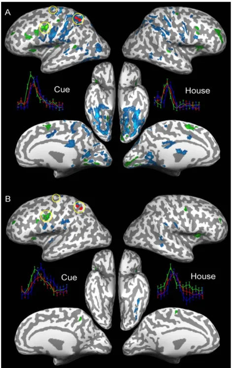
Figs. 4A and B show the dGCMs for a face-selective region in the left infero-temporal cortex, identified by location and selectivity as the fusiform face area (FFA), for subjects 1 and 2, respectively. Regions shown in green have significantly negative influence difference terms and are thus indicated to be sources of influence to the reference ROI. Regions shown in blue have significantly positive influence difference terms and are thus indicated to be targets of influence from the reference ROI. The dGCMs show qualitatively similar patterns of influence from and to the left FFA in the two subjects. A strong influence on the left FFA from early visual areas including the calcarine sulcus can be seen in both subjects. Lateral premotor areas and medial supplementary and pre-supplementary motor areas also show a strong influence on the left FFA. The left FFA itself exerts its influence mainly on other parts of the bilateral infero-temporal cortex and on regions in bilateral posterior parietal cortex (PPC). To aid in the interpretation of the maps, a post hoc deconvolution analysis was performed on the time-courses of selected foci in the maps. Event-related averages are shown for selected regions including the reference ROI, synchronized to the occurrence of the remapping cue and the face stimulus. This post hoc analysis provides valuable insight into the interpretation of the GCMs. It shows that the signal of influence sources in the maps rises and peaks before the signal of the reference region. The signal-rise and signal-peak of the reference region, in turn, precedes those of the influence targets. This observation indicates an agreement between fMRI mental chronometry (Formisano and Goebel, 2003; Menon et al., 1998) and GCM to the extent that the temporal precedence in stimulus-locked signal variation appears to be a contributing factor to the GCMs. It should be noted that GCMs also reflect the
contributions from stochastic signal dependencies that are not strictly stimulus-locked, since they are computed over large time-segments within an experimental run.
An important issue that should be addressed when relying on temporal precedence between fMRI signals from different sites in the brain is the variability of the hemodynamics over the brain (Formisano and Goebel, 2003; Saad et al., 2001). More precisely, one should rule out the possibility that influence found from one area to another based on temporal difference in signal variation is
due to a systematic difference in the hemodynamic lag at the two areas. A possible approach to exclude this confound is to show that the measured influence varies with experimental condition or cognitive context. The reasoning is that structural differences in hemodynamics persist over different conditions or contexts, so that any observed systematic variation with condition or context, should be due to changes in the neuronal population interactions. Thus, in the presence of such experimentally modulated influence, one can more reliably conclude that the measured influences reflect Fig. 4. Thresholded difference GCMs for a face-selective region in the left fusiform gyrus for subject 1 in (A) and subject 2 in (B). The FDR-based threshold was set toq= 0.05. The reference region is shown in red. Green areas have a significant negative difference term and are sources of influence to the reference region. Blue areas have a significant positive difference term and are targets of influence from the reference region. Event-related BOLD responses are shown for the circled areas in the calcarine sulcus (in green), the fusiform gyrus (the reference area, in red) and the intra-parietal sulcus (in blue) for both the Cue stimulus and the Face stimulus. Vertical bars indicate estimated standard errors.
true neuronal interactions. To this end, we investigated differences between the dGCMs found in the fast switching (FS) condition and the slow switching (SS) condition. FS runs were of a similar length as the SS runs and contained a similar number of face, house, and control stimuli. However, the number of switches in the S–R mapping in the FS runs was three times that in the SS runs. Thus, although the stimuli, responses, and the general task were the same in both conditions, the FS runs created a much more engaging context, in which the subjects were required to exert a higher
degree of executive control in order to switch the S–R mapping every few trials. Thus, it was hypothesized that this difference in task requirements and the ensuing cognitive context would be reflected in a difference in interactions between areas that coordinate the required executive control. Figs. 5A and B show, for the FS runs and the SS runs, respectively, the dGCMs for subject 1 for a region in left posterior parietal cortex (PPC), thresholded at the same level. The reference region in left PPC was found to be highly activated at remapping cues, together with
Fig. 5. Thresholded difference GCMs for a region in the left intraparietal sulcus for subject 1 for the fast-switching runs in (A) and the slow-switching runs in (B) as inFig. 4. The FDR-based threshold was set to q = 0.05 for both A and B. Event-related BOLD responses are shown for the circled areas in the inferior part of the left precentral sulcus (in green), the left PPC (the reference area, in red) and the superior part of the left precentral sulcus (in blue) for both the Cue stimulus and the House stimulus.
lateral premotor and prefrontal regions, medial supplementary motor regions and other parietal areas. Overall, the dGCMs for FS runs and SS runs look qualitatively very similar but differ in intensity, suggesting that the degree of interaction of the left PPC with other sites in the brain is different. In the FS runs, the left PPC is seen to be influenced mainly by premotor and prefrontal regions and presupplementary motor regions (left more strongly than right). There is also influence from bilateral insula regions and small clusters around the calcarine sulcus. The left PPC region itself exerts its influence mainly on large parts of the inferotem-poral cortex, lateral motor, and premotor areas and inferior and superior parietal areas. In the SS runs, the influence from some of the premotor, prefrontal, and insula regions remains, though mostly at a lower intensity. The influence from the reference region on some of inferior parietal and inferotemporal regions also remain in the SS runs at a lowered level. Overall, it can be seen that the change in cognitive context strongly modulates the intensity of the maps.Fig. 5A shows the event-related responses for the remapping cue and the house stimulus in the FS runs. These responses reflect the temporal order relations implied by the GCM. InFig. 5B, the lower intensity of the maps in the SS runs is reflected in a less clearly structured relationship between the event-related averages.
Discussion
We have proposed Granger causality mapping (GCM) as an approach to explore directed influences between neuronal populations in fMRI data. The method does not rely on a priori specification of adstructuralTordanatomicalTmodel that contains pre-selected regions and connections between them. This distin-guishes it from other effective connectivity approaches, such as covariance structural equation modeling (McIntosh and Gonzalez-Lima, 1994) and dynamic causal modeling (Friston et al., 2003), that aim at testing or contrasting specific hypotheses about neuronal interactions. Instead, GCM relies on the concept of Granger causality to define the existence and direction of influence between two stochastic time-series purely on the basis of temporal precedence in their interdependency. Granger causality can be formalized and tested using vector autoregressive (VAR) models that capture the joint temporal dynamics of several time-series. Effective connectivity approaches that are based on instantaneous regression equations relating only concurrent values, such as psychophysiological interactions (Friston et al., 1997) and struc-tural equation modeling, discard possibly important temporal information in the data. It has been shown (Lahaye et al., 2003) that even in the context of functional connectivity, incorporating lagged values increases the sensitivity to detect relationships between typical fMRI time-series. Many of the more recent effective connectivity approaches are based on stochastic or deterministic dynamic models, capable of capturing temporal structure. The Volterra series representation (Friston and Buchel, 2000) characterizes interactions in a nonlinear convolution model relating multiple inputs to a single output. Thus dynamic nonlinear influences on a single region can be characterized. In the multivariate context, the vector autoregressive models used by
Harrison et al. (2003)can quantify directed influences between all regions included in the model. Although temporal information is used to give direction to the influences, the set of interacting regions must be chosen beforehand. The same holds for dynamic causal models (Friston et al., 2003) that use deterministic
state-space models to represent neuronal dynamics and interactions augmented with forward models of the regional hemodynamic response. Pre-specified models are very useful, even necessary, when a specific hypothesis about neuronal interactions must be tested. Furthermore, most methods making use of a predefined anatomical model, capture the dynamics of all included regions simultaneously in a full multivariate model. This allows them to characterize and infer on indirect influences and other more complicated influence pattern than the canonical done-to-manyT pattern inherent to the (bivariate) Granger Causality Mapping approach presented here. However, inference on a hypothesis concerning part of the specified network is very sensitive to misspecification of the model. Especially, the omission of areas or structures that mediate influences or form an additional source of influence can lead to spurious interactions. Furthermore, in early stages of investigation, specific hypotheses about the exact network underlying performance of a cognitive task might not be readily available. As an exploratory method, Granger causality mapping can form an important complement to these hypothesis-driven methods in helping to formulate directed graph models of regions and their interactions.
The fMRI signal is influenced by the intervention of hemodynamics and a relatively low temporal resolution with respect to the interactions of neuronal populations. Simulations showed that these intervening operations of low-pass filtering and down-sampling can introduce bias in inference on ordinary granger causality based statistics. However, it was shown that robust detection of unidirectional influence from one neuronal population to another is possible in the fMRI signal using the proposed influence-difference term. Interestingly, with sufficiently high sample rates high sensitivity could be obtained even for influences with moderate strength and delay, suggesting that in practice considerable power could be gained with faster acquisition schemes. In resolving unidirectional influences based on temporal precedences in signal fluctuations, Granger causality mapping relates to the approach of fMRI mental chronometry (Formisano and Goebel, 2003; Menon et al., 1998). In fMRI mental chronometry, the onset latency of BOLD responses is used to resolve a sequence of processing stages. Granger causality mapping forms an extension to this method, in principle using temporal precedence not only in the stimulus locked onset of the BOLD response but also in the ongoing signal fluctuations. Indeed, we observed that the latency of trial-based BOLD responses largely agreed with the directionality discovered by the GCMs. An interesting question arising from these observa-tions is to what amount the influences found are driven more by strictly stimulus-locked deterministic signal fluctuations or by ongoing stochastic fluctuations, perhaps more indirectly induced by the experimental design. By its very nature, an autoregressive model does not distinguish between these two sources of signal fluctuations. The dynamics of the signal-fluctuations in an autoregressive model are driven by the random error process
u[n], which is therefore often called the innovation process. The causes of the fluctuations in the innovation-process itself are not explicitly modeled and, therefore, remain unclear after the fitting of an autoregressive model to given data. Thus, it is only by the post hoc deconvolution analysis that we could ascertain that stimulus-locked signal changes, as characterized by an event-related average, seem to be an important source of temporally delayed signal fluctuations captured by the autoregressive models. More generally, autoregressive models estimated on the fMRI
signal do not allow adblind deconvolutionT that reconstructs an estimate of neuronal population dynamics (e.g., LFPs) from the observed fMRI signal. This would require more complex models with physiologically feasible state-variables and parameters, and an invertible observation model that characterizes local hemo-dynamics (Friston et al., 2003; Riera et al., 2004).
A question that remains is how influence difference terms can be interpreted in the context of more complicated bi-directional interactions, such as top-down feedback. Consider, for instance, a cortical area that sends bottom-up influence to a down-stream region and simultaneously receives top-down modulation from that same area. In this case, a dGCM likely shows only the dominant direction of influence, and only has the capacity to detect changes in the dominant direction of information flow between tasks or conditions. However, in a slightly different case where the source of bottom-up influence and the target of top-down modulation are different but anatomically very close, the exploratory mapping approach can prove to be very useful. With sufficient spatial resolution, a dGCM can identify and distinguish these functionally different parts of the network that might otherwise have been lumped together.
An important consideration in any method that relies on temporal precedence in fMRI data is to discount systematic differences in the lag of the BOLD response as a cause of the results. Of primary concern here is the possibility of a systematic difference in the lag of the hemodynamic response between different brain structures. Such a systematic difference could yield spurious influences. We examined the modulation of influence by experimental demands and cognitive context as a way to rule out hemodynamics as a cause of the results. The pattern of influences for a left posterior parietal region was indeed shown to be modulated by a change to an experimental context that required less cognitive effort. Perhaps, explicit modeling of these modu-lations as psychophysiological interactions in a dynamic context (Friston and Buchel, 2000; Harrison et al., 2003) can form a useful extension to the current approach. A possible further improvement in the applicability of the method is its combination with approaches that try to identify and remove the effects of large draining vessels in fMRI data. Large vessels could often be observed in the GCMs, especially before projection onto the cortical surface. There is certainly an influence from the hemodynamic signal measured in a cortical area to that of the vessels that drain it. However, since in neuroimaging studies it is generally the interactions between neuronal populations that are of interest, strategies to remove vessel-related effects from the GCMs would be a useful addition. One should consider that in the current implementation of GCM, one cannot be absolutely certain that a detected influence between two areas is a direct influence. This means that the influence shown between two cortical regions in a dGCM could run via a third region. However, in this case, the third region would also be expected to show up in the same map. In addition, computation of an additional dGCM with this region as the reference could reveal its intervening role, being a target of influence from one of the areas, and a source of influence to the other. Similar considerations apply for other situations with additional influence from areas not taken into account, such as cases of common input. Computing conditional GCMs based on conditional influence measures (Geweke, 1984), which include the activity of a third area into the VAR models to partial out its influences, is a possible further approach towards handling these cases.
In summary, we think the exploratory approach of mapping influences between a region of interest and the rest of the brain will form a very useful addition to existing models of effective connectivity. The absence of structural assumptions in the form of an anatomical model makes it a useful tool in exploring possible alternative anatomical models underlying performance of cognitive and sensorimotor tasks. Because of its reliance only on assump-tions incorporated in the concept of Granger causality, it can clarify which interactions are supported by temporal precedence informa-tion in the acquired data, and which other interacinforma-tions, highlighted only by instantaneous correlations, require explicit directional modeling. Especially in early phases of investigation and data analysis, our method can help formulate explicit hypotheses about functional networks that can later be tested with more hypothesis-driven approaches.
Acknowledgment
This work was supported by the Human Frontiers Science Program.
Appendix A. Computation of the influence measures
Geweke’s dependence measure Fx,y (Geweke, 1982) can be
defined using the (zero-lag) autocorrelation matrices of the residuals of the following three VAR models involving the K-dimensional seriesx[n] and L-dimensional seriesy[n]:
x½ ¼ n X p i¼1 Ax½ ix½ni þu½ n varðu½ nÞ ¼1 y½ ¼ n X p i¼1 Ay½ iy½ni þv½ n varðv½ nÞ ¼T1 and withq½ ¼n x½ n y½ n : q½ ¼ n X p i¼1 Aq½ iq½ni þw½ n varðw½ nÞ ¼Y¼ 2 C CT T 2
whereq[n] isO-dimensional (withO=K+L),1and2areK
byK,T1andT2areLbyL, andYisObyO. Although bothx[n]
andy[n] can both be vector time series, they were both scalar time series in these investigations, that is, K = L = 1. The residual correlation matrices1,2, andY, quantify how well we are able
(using linear AR models) to predict current values ofxandyfrom their past values. The measures of total linear dependence between xandy, linear influence fromxtoy, linear influence fromytox, and instantaneous influence between x and y are defined to be, respectively (Geweke, 1982):
Fx;y¼lnðj1jdjT1j=jYjÞ
FxYy¼lnðjT1j=jT2jÞ
FyYx¼lnðj1j=j2jÞ
where || is the determinant of. From these definitions, it can be seen that it holds that:
Fx;y¼FxYyþFyYxþFxSy
Here, we are assuming that the finite order AR-models are valid descriptions of the time-series x[n], y[n], and q[n], which also implies the assumption thatq[n] is wide sense stationary (WSS) and thus thatx[n] andy[n] are jointly WSS. Since it holds that |T2|V|T1|,FxYywill always be nonnegative. As we can interpret
the determinant of a correlation or covariance matrix as a measure of generalized variance, |T1| is the generalized variance of the
mean squared error in predictingy[n] by a linear projection on its own past values {y[n1],y[n2], . . .}. Therefore,FxYyquantifies
the reduction in this generalized variance obtained by adding past values ofxto the projection set. A similar interpretation holds for FyYx .Fxdy essentially quantifies the deviation of the residual
correlation matrixYof the joint VAR model from being block-diagonal, and thus the extent to which there is residual instanta-neous correlation betweenx[n] andy[n].
VAR models were estimated from simulated or experimental data using a version of the multivariate fast orthogonal algorithm specialized for the estimation of VAR models with the possibility for non-linear terms and time-varying coefficients (Bagarinao and Sato, 2002). To specify the orderpof the autoregressive models to be estimated, the Schwarz Criterion (SC) was used, which is an order selection criterion, constructed in a Bayesian context that trades off reduction in error-variance against increased model complexity, that is, number of parameters (Luetkepohl, 1991). The SC for a given VAR model fit is a function of model orderp, model dimensionD, the residual correlation matrix, and the number of observations N, and is given as SC pð Þ ¼lnðjjÞ þlnð ÞN
N pD
2
(Luetkepohl, 1991), where djjT denotes the determinant of . Evaluating SC(p) for a large range of orders, the optimal order is selected as that for which SC(p) is minimal.
Appendix B. Statistical inference
Parametric inference was developed for the influence measures FxYy,FyYx, andFxdy (Geweke, 1982). However, such inference
does not extend to more general conditional measures of influence (Geweke, 1984), and is not valid when dealing with sampled or aggregated time-series (Wei, 1990). Thus, inference on computed influence measures was performed within the framework of the bootstrap methodology (Efron and Tibshirani, 1993). A large number M of surrogate time-series are generated that are sufficiently dlikeT the original in their dynamic and statistical properties and that satisfy the null hypothesis of no influence. Computation of the influence measures over these surrogates gives a bootstrap empirical distribution of values that characterizes the null hypothesis. The empirical P value or achieved significance level (ASL) for a given influence statistic obtained from real data can be taken as the proportion of values in the empirical null distribution more extreme than this value. Inference can then proceed either within the classical framework, controlling for probability of type I error a or, alternatively, with methods controlling for the False Discovery Rate (FDR). A classical test for an influence term being larger than zero is performed by setting the significance threshold at the value in the empirical null distribution that separates thea*M largest values from the rest. A two-sided
test for an influence difference termFxYyFyYx(see text) being
non-zero corresponds to setting a lower threshold at the value in the empirical null distribution of difference terms that separates the (a/2)*Msmallest values from the rest, and a upper threshold at the separation of the (a/2)*Mlargest values.
When performing a large numberVof simultaneous statistical tests (e.g., over a large number of voxels in a statistical parametric map), one can alternatively employ methods that control for the FDR, the expected proportion of false positives among all tests for which the null hypothesis is rejected (Genovese et al., 2002). This has the advantage of dealing with multiple comparison problem, while retaining considerable power in the detection of effects and adapting to the noise level in the data. The FDR-based thresholds corresponding to a two-sided test for the influence difference term being non-zero at an accepted FDR levelqare obtained from the set of empirical P values of the obtained statistics over all voxels. EmpiricalPvalues for the influence difference terms were pooled for positive and negative terms by taking absolute values of both the true statistic distribution and the null distribution. The empiricalP value for a given (absolute) difference term was then obtained as the proportion of larger values in the (absolute) empirical null distribution. Subsequently, the FDR-based threshold is obtained from thePvalues as follows. In the ordered collection ofPvalues, let r be the largestifor which P[i]V(i/V) * (q/c(V)), then the threshold is set at the value corresponding to thePvalue P[r]. The value of the constant c(V) is determined by assumptions on the joint distribution ofPvalues over all voxels. Here, it was set toc(V) = 1, which applies when thePvalues at different voxels are independent and when noise is Gaussian with nonnegative correlation across voxels. Alternatively, it can be set to c Vð Þ ¼V
i¼11=i; which
applies for any distribution ofPvalues over voxels.
References
Baccala, L.A., Sameshima, K., 2001. Partial directed coherence: a new concept in neural structure determination. Biol. Cybern. 84, 463 – 474. Bagarinao, E., Sato, S., 2002. Algorithm for vector autoregressive model parameter estimation using an orthogonalization procedure. Ann. Biomed. Eng. 30, 260 – 271.
Bernasconi, C., Konig, P., 1999. On the directionality of cortical interactions studied by structural analysis of electrophysiological recordings. Biol. Cybern. 81, 199 – 210.
Bernasconi, C., von Stein, A., Chiang, C., Koenig, P., 2000. Bi-directional interactions between visual areas in the awake behaving cat. Neuro-Report 11, 689 – 692.
Boynton, G.M., Engel, S.A., Glover, G.H., Heeger, D.J., 1996. Linear systems analysis of functional magnetic resonance imaging in human V1. J. Neurosci. 16, 4207 – 4221.
Brovelli, A., Ding, M., Ledberg, A., Chen, Y., Nakamura, R., Bressler, S.L., 2004. Beta oscillations in a large-scale sensorimotor cortical network: directional influences revealed by Granger causality. Proc. Natl. Acad. Sci. U. S. A. 101, 9849 – 9854.
Buchel, C., Friston, K.J., 1997. Modulation of connectivity in visual pathways by attention: cortical interactions evaluated with structural equation modelling and fMRI. Cereb. Cortex 7, 768 – 778.
Efron, B., Tibshirani, R.J., 1993. An Introduction to the Bootstrap. Chapman and Hall, New York.
Epstein, R., Kanwisher, N., 1998. A cortical representation of the local visual environment. Nature 392, 598 – 601.
Formisano, E., Goebel, R., 2003. Tracking cognitive processes with functional MRI mental chronometry. Curr. Opin. Neurobiol. 13, 174 – 181.
Freiwald, W.A., Valdes, P., Bosch, J., Biscay, R., Jimenez, J.C., Rodriguez, L.M., Rodriguez, V., Kreiter, A.K., Singer, W., 1999. Testing non-linearity and directedness of interactions between neural groups in the macaque inferotemporal cortex. J. Neurosci. Methods 94, 105 – 119.
Friston, K., 1994. Functional and effective connectivity in neuroimaging: a synthesis. Hum. Brain Mapp. 2, 56 – 78.
Friston, K., 2002. Beyond phrenology: what can neuroimaging tell us about distributed circuitry? Annu. Rev. Neurosci. 25, 221 – 250.
Friston, K.J., Buchel, C., 2000. Attentional modulation of effective connectivity from V2 to V5/MT in humans. Proc. Natl. Acad. Sci. U. S. A. 97, 7591 – 7596.
Friston, K.J., Frith, C.D., Frackowiak, R.S.J., 1993a. Time-dependent changes in effective connectivity measured with PET. Hum. Brain Mapp. 1, 69 – 79.
Friston, K.J., Frith, C.D., Liddle, P.F., Frackowiak, R.S.J., 1993b. Func-tional connectivity: the principle component analysis of large (PET) data sets. J. Cereb. Blood Flow Metab. 13, 5 – 14.
Friston, K.J., Buechel, C., Fink, G.R., Morris, J., Rolls, E., Dolan, R.J., 1997. Psychophysiological and modulatory interactions in neuroimag-ing. NeuroImage 6, 218 – 229.
Friston, K.J., Harrison, L., Penny, W., 2003. Dynamic causal modelling. NeuroImage 19, 1273 – 1302.
Genovese, C.R., Lazar, N.A., Nichols, T., 2002. Thresholding of statistical maps in functional neuroimaging using the false discovery rate. NeuroImage 15, 870 – 878.
Geweke, J.F., 1982. Measurement of linear dependence and feedback between multiple time series. J. Am. Stat. Assoc. 77, 304 – 324. Geweke, J.F., 1984. Measures of conditional linear dependence and
feedback between time series. J. Am. Stat. Assoc. 79, 907 – 915. Goebel, R., Roebroeck, A., Kim, D.S., Formisano, E., 2003. Investigating
directed cortical interactions in time-resolved fMRI data using vector autoregressive modeling and Granger causality mapping. Magn. Reson. Imaging 21, 1251 – 1261.
Goebel, R., Roebroeck, A., Kim, D.S., Formisano, E., 2004. Directed cortical interactions during dynamic sensory-motor mapping. In: Duncan, J. (Ed.), Attention and Performance XX. Oxford University Press, New York, pp. 439 – 462.
Granger, C.W.J., 1969. Investigating causal relations by econometric models and cross-spectral methods. Econometrica 37, 424 – 438. Granger, C.W.J., 1980. Testing for causality: a personal viewpoint. J. Econ.
Dyn. Control 2, 329 – 352.
Harrison, L., Penny, W.D., Friston, K., 2003. Multivariate autoregressive modeling of fMRI time series. NeuroImage 19, 1477 – 1491. Hesse, W., Moller, E., Arnold, M., Schack, B., 2003. The use of
time-variant EEG Granger causality for inspecting directed inter-dependencies of neural assemblies. J. Neurosci. Methods 124, 27 – 44.
Horwitz, B., 1990. Simulating functional interactions in the brain: a model
for examining correlations between regional cerebral metabolic rates. Int. J. Biomed. Comput. 26, 149 – 170.
Horwitz, B., Grady, C.L., Haxby, J.V., Ungerleider, L.G., Schapiro, M.B., Mishkin, M., Rapoport, S.I., 1992. Functional associations among human posterior extrastriate brain regions during object and spatial vision. J. Cogn. Neurosci. 4, 311 – 322.
Kaminski, M., Ding, M., Truccolo, W.A., Bressler, S.L., 2001. Evaluating causal relations in neural systems: granger causality, directed transfer function and statistical assessment of significance. Biol. Cybern. 85, 145 – 157.
Kanwisher, N., McDermott, J., Chun, M.M., 1997. The fusiform face area: a module in human extrastriate cortex specialized for face perception. J. Neurosci. 17, 4302 – 4311.
Kay, S.M., 1988. Modern Spectral Estimation: Theory and Application. Prentice Hall, Englewood Cliffs, NJ.
Kriegeskorte, N., Goebel, R., 2001. An efficient algorithm for topologically correct segmentation of the cortical sheet in anatomical mr volumes. NeuroImage 14, 329 – 346.
Lahaye, P.J., Poline, J.B., Flandin, G., Dodel, S., Garnero, L., 2003. Functional connectivity: studying nonlinear, delayed interactions between BOLD signals. NeuroImage 20, 962 – 974.
Liu, H., Gao, J., 2000. An investigation of the impulse functions for the nonlinear BOLD response in functional MRI. Magn. Reson. Imaging 18, 931 – 938.
Logothetis, N.K., Pauls, J., Augath, M., Trinath, T., Oeltermann, A., 2001. Neurophysiological investigation of the basis of the fMRI signal. Nature 412, 150 – 157.
Luetkepohl, H., 1991. Introduction to Multiple Time Series Analysis. Springer-Verlag, Heidelberg.
McIntosh, A.R., Gonzalez-Lima, F., 1994. Structural equation modeling and its application to network analysis in functional brain imaging. Hum. Brain Mapp. 2, 2 – 22.
McIntosh, A.R., Grady, C.L., Ungerleider, L.G., Haxby, J.V., Rapoport, S.I., Horwitz, B., 1993. Network analysis of cortical visual pathways mapped with PET. J. Neurosci. 14, 655 – 666.
Menon, R.S., Luknowsky, D.C., Gati, J.S., 1998. Mental chronometry using latency-resolved functional MRI. Proc. Natl. Acad. Sci. U. S. A. 95, 10902 – 10907.
Riera, J.J., Watanabe, J., Kazuki, I., Naoki, M., Aubert, E., Ozaki, T., Kawashima, R., 2004. A state-space model of the hemodyna-mic approach: nonlinear filtering of BOLD signals. NeuroImage 21, 547 – 567.
Saad, Z.S., Ropella, K.M., Cox, R.W., DeYoe, E.A., 2001. Analysis and use of fMRI response delays. Hum. Brain Mapp. 13, 74 – 93. Talairach, J., Tournoux, P., 1988. Co-planar Stereotaxic Atlas of the Human
Brain: 3-Dimensional Proportional System, an Approach to Cerebral Imaging. Thieme, Stuttgart.
Wei, W.W.S., 1990. Time Series Analysis: Univariate and Multivariate Methods. Addison-Wesley, Redwood City.