AN INVESTIGATION INTO THE HEDONIC PRICE ANALYSIS OF THE STRUCTURAL CHARACTERISTICS OF RESIDENTIAL PROPERTY IN THE
WEST RAND
ROBERT SCOTT DODDS
A research report submitted to the Faculty of Engineering and the Built Environment, University of the Witwatersrand, in fulfillment of the requirements of the degree of Master of Science in Building.
ABSTRACT
A vast amount of literature on hedonic price modelling has been formulated on overseas property markets. Very little currently exists in South Africa and this poses a risk for sellers and estate agents of a residential property when listing it on the open market, as this could result in an extended list period, reducing the original asking price. This paper seeks to examine Gauteng’s West Rand residential property market and formulate a multi-variate regression model to best predict property prices, determined by a property’s structural characteristic. The research tracks residential sales from 1996 to 2009, a
thirteen-year sample period from which a composite property index, to account for inflation and real house price growth, has been formalised. Correlation and regression analysis was used to interpret the data at the relevant significance level. In order to account for locational attributes present in property values, the data set was divided into locational quadrants and run as dummy variables. A further regression was run on a screened data set to create an ordinary least squares equation that could be used to show the relationship between property values and structural characteristics. The results indicated a good fit with an R2 of 69.5%. This regression was then applied practically to predict property prices for houses that have transacted in the West Rand property market, and plotted along a value/price graph using the 45-degree true value frontier line. The relevant results were then interpreted, and recommendations given.
DECLARATION
I declare that this research report is my own unaided work. It has been submitted for the Degree of Master of Science in Building in the University of the Witwatersrand,
Johannesburg. It has not been submitted before for any degree or examination in any other University.
_________________________ (Signature of Candidate)
TABLE OF CONTENTS
ABSTRACT ... i
TABLE OF CONTENTS ... iii
LIST OF FIGURES ... v
LIST OF TABLES ... vi
1. INTRODUCTION... 1
1.1. Background to the study ... 2
1.2. Research Question... 4
1.3. Statement of the problem ... 4
1.4. Statement of thesis ... 5
1.5. Sub problems ... 5
1.6. Significance of the study ... 6
1.7. Scope and delimination of work ... 7
1.8. Assumptions ... 7
1.9. Structure of the report ... 8
2. LITERATURE REVIEW ... 9
2.1. Introduction ... 9
2.3.1. Advantages and disadvantages ... 20
2.3.2. Present day hedonic price modelling ... 22
2.4. Conclusion ... 26 3. RESEARCH METHODOLOGY ... 28 3.1. Types of research ... 28 3.1.1. Structured research ... 28 3.1.2. Unstructured research ... 29 3.2. Sample frame ... 31 3.3. Correlation analysis... 33 3.4. Regression analysis ... 34 3.5 Regression application ... 38
4. RESEARCH DATA, EMPERICAL RESULTS AND ANALYSIS ... 39
4.1. Data capture ... 39 4.2. Data adjustment... 39 4.3. Descriptive statistics ... 44 4.3.1. Quantitative variables ... 44 4.3.2. Qualitative variables ... 45 4.4. Correlation analysis... 46 4.5. Regression analysis ... 49
4.5.1. Structural attributes on the full data set... 49
4.5.2. Structural variables and area groupings ... 62
4.5.3. Structural attributes for selected pocket of suburbs ... 65
4.6. Application of the model for the entire West Rand region ... 69
5. CONCLUSION ... 72
6. RECOMMENDATIONS ... 74
7. REFERENCES ... 75
LIST OF FIGURES Figure 4.1 Average house price growth for the West Rand ...42
Figure 4.2 Heteroscedasticity for data set Table 4.8 ...54
Figure 4.3 Histogram of residual error for data set Table 4.8 ...55
Figure 4.4 Normal Probability Plot of residual error for data set Table 4.8 ...56
Figure 4.5 Heteroscedasticity for data set Table 4.8 ...59
Figure 4.6 Histogram of residual error for data set Table 4.8 ...60
LIST OF TABLES
Table 4.1 Summary of West Rand house growth data ...41
Table 4.2 Summary statistics of regression variables ...44
Table 4.3 Number of observations for each region comprising the West Rand ...45
Table 4.4 Number of observations for each qualitative factor ...45
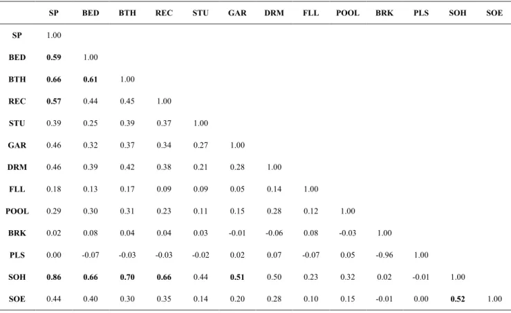
Table 4.5 Correlation matrix of structural variables for West Rand ...46
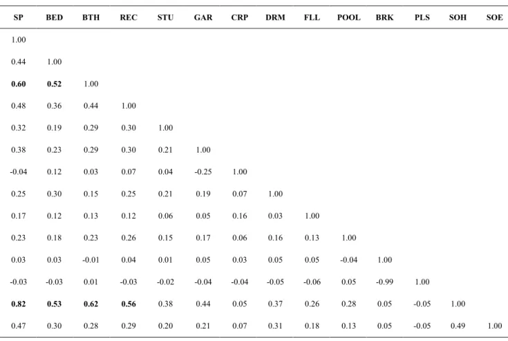
Table 4.6 Correlation matrix of structural variables for pocket suburbs ...48
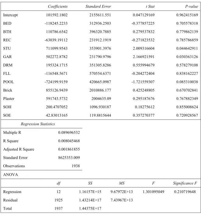
Table 4.7 Regression output: included observations = 1 938 ...50
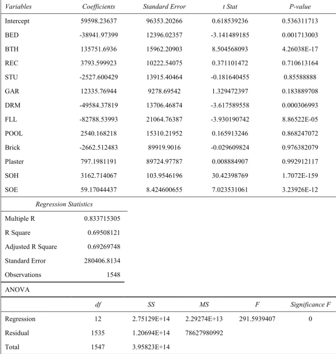
Table 4.8 Regression output: included observations = 1 548 ...52
Table 4.9 Regression output: Log of Adjusted SP included observations = 1 548………….…...58
Table 4.10Regression output: included observations = 1 548 ...63
Table 4.11Regression output: Included observations = 1 548 ...64
1. INTRODUCTION
South Africa has experienced a massive growth rate in prices of housing over the past several years. Understanding these price changes is important for several reasons. Residential housing serves as a big source of an individual’s wealth and any changes in the underlying value of a house dramatically affects one’s consumer spending and savings decisions. This, in turn, has an overall affect on economic activity. It is therefore important to have an accurate measure of aggregate housing prices (Rappaport, 2007). The sale of a residential house involves strategic interaction between a seller and a set of potential buyers. When a house is listed on the market, the seller advertises a certain listing price (usually through a property agent) and awaits a potential offer from a buyer. The listing price will influence the arrival of offers, which will determine the date on which the sale is concluded. As the time the property is on the market increases, the arrival rate of potential buyers decreases, and the probability of the listing price changing increases.
If the original asking price is high, the sale price is usually relatively high, but also experiences a longer time on the market (Ortalo-Magne, 2002). Taking the above into account, the pricing of a house sale is important.
This research analyses the structural determinants of residential property in Gauteng’s West Rand, and develops a hedonic pricing model with statistical significance that could reasonably explain the open market value of a residential house, given a set of structural variables.
1.1. Background to the study
According to Hill and Melser (2008), who conducted research in Sydney Australia, using housing data for 14 regions over six years, existing house price indices usually measure the average or median price of houses sold during a given period of time. The problem with this method is that the mix of houses sold could change dramatically over time. For a price index to be useful, it must compare the sales of equivalent houses from one period to the next.
When interviewed on 20 June 2009, Mrs. N. Vergotine-Dube1 confirmed that, in South Africa, several property house price indices are available. One of the most popular indices used amongst property valuers and bankers is that of the South African Property Transfer Guide (SAPTG). This is an online property sales registry that records all
transactions registered in the South African Deeds Office. This information is useful as it illustrates sales volume and house price trends over a given period.
Other indices used in the business world to monitor house price growth, according to Mrs. N. Vergotine-Dube during an interview held on 20 June 2009, include the African Bank South Africa (ABSA), First National Bank (FNB), and Standard Bank of South Africa (SBSA), property indices. These indices use either the mode, median or mean to calculate the average increase in property prices, and would include repeat sales of an equivalent nature.
Previous models tried to overcome this problem by only dealing with repeat sales
1
occurring during the specific time set. This method was seen as an improvement on the average price approach but was still littered with problems (Hill and Melser, 2008). (Hill and Melser, 2008) listed the following problems with the repeat sales method:
• It cannot account for spatial price indices as the same house could not sell twice during a given period in a different place;
• the maximum use of available data is not utilized as houses that do not sell twice during a period are omitted;
• data captured earlier on needs to be updated as new data is forever being created;
• the possibility of a property’s condition being the same when it is sold for the second time during a particular period, several years since the initial sale, is difficult to guarantee as the model does not account for depreciation; and
• repeat sales data may tend to differ from single sale data as they may not follow the same sale path (e.g. flats could take longer to sell than houses) and different sales classes’ (flats verses house) prices may tend to grow at different rates, resulting in the index becoming biased.
According to Hill and Melser (2008) a hedonic approach to house price construction has the potential to resolve the issues highlighted above and significantly improve the quality of house price valuation. The essence behind such an approach is to regress the price of the house in terms of its characteristics. This method has emerged as the general one used within the property industry for measuring the housing market.
According to Keng (1997), who conducted studies on the Malaysian property market from 1988 to 1997 using correlation and regression analyses to create a housing price index, no two houses are alike due to their heterogeneity, and house prices differ
Keng (1997) mentions that in order to indicate the price variations in the individual attributes from one house to the next, the price measure must be segregated. Multiple regression analysis (MRA) enables the estimation of changes in average price from one time period to another on a standardised basis, and hence forms the hedonic function.
1.2. Research Question
The research has asked: What statistically significant structural characteristics of a residential house will determine the open market value? The research examined the sales recorded by estate agents in relation to each property’s structural characteristic, and found a solution to this question.
1.3. Statement of the problem
The problem statement to be addressed in this research study may be stated as:
Do the structural characteristics of a residential house determine its open market value, and if so, are they statistically significant?
Further, the research will also probe into the potential effects location will have on the selling price of a house.
The reason the above problem statement is being researched is for the investigation into an alternative method of property valuation that can replace the need for a physical inspection by a property valuer. This is because before a bank will bond and grant a loan on a property, it must assess the property’s market value.
Under normal banking circumstances, a bank will acquire the expertise of a professional property valuer to conduct a physical property inspection of the property in question and write a report on its perceived market value.
Besides the time required for a property valuer to inspect and write up the report, which wastes valuable time for the bank and purchaser, a cost is attached to the creation of the property valuation report.
The West Rand is one of the more established residential areas in Johannesburg where property price ranges are not extreme, and property characteristics are fairly
homogenous. The West Rand is one of Johannesburg’s largest residential areas and would therefore comprise a big portion of any banks loan book. Bearing this in mind, it is seen as prudent that a hedonic model is created for banks to utilise when valuing property in the West Rand, to cut down on costs, and reduce turnaround times when allocating bonds.
1.4. Statement of thesis
The structural characteristics of a residential property will influence its open market value, and a basic multi-variate linear regression model can be used to estimate a property’s value within certain bounds, given a set of statistically significant structural variables.
1.5. Sub problems
Sub problems were created in order to break the main research question down into constituent parts, for which workable solutions could be formulated. The following sub-problems were researched:
• Does the stand size of a property affect the open market value?
• Does the dwelling size of a property affect the open market value?
• Does the number of recreational rooms affect the open market value?
• Does the number of study rooms affect the open market value?
• Does a garage affect the open market value?
• Does the wall type of the property affect the open market value?
• Does the location of the property affect the open market value?
1.6. Significance of the study
When interviewed on 20 June 2009, Mrs. N. Vergotine-Dube confirmed that there is awareness amongst professionals within the property environment, that automated
valuation reports generated for a residential property, rely on insignificant sales data. This poses a risk for sellers and estate agents of a residential property when listing it on the open market as this could result in an extended list period, reducing the original asking price.
Mrs. N. Vergotine-Dube further commented that risks are also extended to banks during a bond grant as the underlying security of the asset, calculated by the automated valuation report, is not always representative of the property’s true open market value, and hence, the bank is under-or-over secured on the property. The spin-offs from this are that the client’s loan to value, exposure and facility are calculated incorrectly, creating
unnecessary risk for both parties.
This study investigates which structural characteristics of a residential property have a significant impact on the open market value, and develops a theoretical marginal value for each of the variables.
Once this is created, the model can be applied to properties currently on the market and help banks to hedge their risk further by identifying over or under capitalised market property transactions.
1.7. Scope and delimination of work
The property industry consists of many different types of transactions, mainly including residential, commercial, retail and industrial. Furthermore, these types can be broken up into different zoning categories which stipulate the certified rights attached to the property. This study focuses mainly on single residential property sales that have ‘residential one’ zoning. The study focuses initially on residential sales that have taken place in Gauteng’s West Rand.
1.8. Assumptions
In a telephonic discussion held with Christo Wiid (16 March 2009)2, Wiid reported that the following assumptions are well researched.
• That Property24.com’s database is accurate.
• That Property24.com’s reporting is in line with the rest of the property industry.
• That the database only contains data for single residential property zoned residential one.
According to Wiid, only data relating to actual sales of single residential properties within the West Rand are recorded in the excel database. Property estate agents responsible for the sale capture the information recorded. Wiid’s final comments were that all empty fields within the spreadsheet can be treated as zeros (or are non-existent characteristics of the property in question).
1.9. Structure of the report
Following the above introduction, a review of past and present literature relating to hedonic price modelling is discussed.
The literature review will summarise some of the first multi-variate experiments carried out on the structural attributes and their affects on property prices, followed by the latest hedonic price analyses of the effects that schools, pollution and greenbelts have on property values.
After the theoretical background has been concluded, an in-depth outline of the methodology to be utilised for the purposes of this thesis is explained, which include correlation and regression analysis. The regression and correlation analysis employed for the purposes of testing the data included four separate statistical tests.
The final regression, which resulted in the highest regression (R2), was then used to formulate the value/price chart to test the data against the 45-degree true value frontier. Upper and lower bounds were included to account for the standard error present in the model.
Finally, concluding remarks regarding the findings are summarised, and recommendations to improve further hedonic price analysis are given.
2. LITERATURE REVIEW
2.1. Introduction
After analysing studies carried out by Ball (1973), Bover and Velilla (2002) and Hill and Melser (2008) the last forty years has seen extensive research into property valuation methods using statistical models.
The initial studies employed techniques such as multiple regression, R² for best fit equation, ordinary least squares (OLS), and certain log equations used to estimate house prices. Since then, general views regarding residential property values have been
formulated relating to location, micro-economy (demand and supply), general macro-economic climate, accessibility and environmental issues.
To date, research within a South African property context is sparse. The journals and sources researched in order to find data on hedonic models and regressions analysis’s, proved fruitless. The main search engines included the following: Sabinet, Emerald, EBSCOhost Web, J Stor and Google Scholar.
Research of existing literature and the study of a hedonic price analysis of the structural characteristics of residential property in Gauteng, is considered value add for the model’s potential use, amongst individuals and companies within the property industry. The following pages delve into previous research, and the lessons learnt for hedonic price modelling.
The only information on hedonic data sourced within a South African context was a study conducted by Van Rensburg et al (2004). The objective of the study was to provide a
One of the issues highlighted in the paper is that the price of something is what you pay, and the value is what you get.
The paper based the regression on the premise that an informed consumer would 1) measure, and 2) maximise the value obtained for each unit of money spent. This was graphically depicted on a graph in their conclusion using a value frontier for red wines farmed in the Western Cape to illustrate wines that were either over priced, or under priced (Van Rensburg et al, 2004). Van Rensburg et al (2004) used price as the dependent variable and regressed it against the independent variables wine type, quality, area of origin, percentage of red wine made by estate, type of wine-firm structure and size of farm. The independent variables or explanatory variables included in the regression were only included if they were perceived to add value to the
consumer.
The term “hedonics” is derived from the Greek word hedonikos, which simply means pleasure. In an economic sense, it refers to the utility or satisfaction one derives through the consumption of goods and services (Leong, 2002).
According to Kathleen et al (2006), it is presumed that humans locate properties that have desirable characteristics (this would include land services), and go on to purchase the property with the most desirable set of structural characteristics. Further comments indicate that the variation in purchase prices and housing characteristics allows for a person’s estimation of the price placed on individual characteristics.
According to Kathleen et al (2006), hedonic models are based on Lancaster’s 1966 theory of consumer demand, where the price of a house is a function of a multitude of attributes. The application of a hedonic price model would therefore estimate the value placed on the different attributes present in a house, and then calculate the property’s overall value.
According to Kathleen et al (2006) the property selected by an individual is a result of the satisfaction they would derive from it. Satisfaction would relate to the use a person could get out of the property.
In economics, satisfaction is known as ‘utilisation’ (Wikipedia, 2009). Therefore, as the number of bedrooms and bathrooms within a property increases, so would the utilisation an individual could gain from the property.
Furthermore, it is common property knowledge that as the number of bedrooms and bathrooms within a property increases, so does the price. Therefore, in order for an individual to gain maximum utility from a property, they would have to balance the satisfaction they expect to gain from it alongside the money they expect to pay.
2.2. History, theory and construction of hedonic price modelling
From the majority of the readings researched, Griliches is mentioned as being the pioneer in hedonic pricing techniques and research. His 1971 work is referenced most frequently. Gressel et al (1984) refers to Griliches being responsible for the initial formulation of the hedonic pricing model.
Goodman (1978) mentions that hedonic price approaches, as noted by Griliches, are based on the premise that a large number of models of a particular heterogeneous commodity can explained by a smaller number of attributes. The equation described is illustrated as follows:
P = f (C) where,
The equation above sets out a very standard MRA. Mark (1988) highlights that an assumption of the above equation is that none of the independent variables are perfectly correlated with the dependant variable.
In a study carried out by Garrod and Willis (1992) on the environmental economic impact of woodland in Britain, they broke down the formation of a hedonic model into six
specific stages. They mentioned that the hedonic model is used to estimate the implicit prices of a set of characteristics which differentiate between similar products in a particular product class.
Therefore, in order to apply this model to the property market, a set of structural and locational characteristics which define a house, and possibly influence its selling price, must be identified.
Dummy variables, or free variables as described by Garrod and Willis (1992), are variables that are known to affect property values, but are of no special interest to the study.
In the study carried out by Garrod and Willis (1992), only a few dummy variables were included in the regression model (such as socio-economic and locational factors). It was highlighted that the omission of such variables in the regression analysis did not affect the results sufficiently enough to warrant their inclusion.
Brown (2004) wrote a paper on hedonic regression models for the Bureau of Labour Statistics in the United States of America to help them meet their current and future needs in terms of the ever-evolving consumer price index. When deciding on the
representatives of the data, Brown (2004) mentions that it is best to split the data into two issues.
The first issue is to decide on whether the data is representative of the market. It is mentioned however that if the representatives selected are not exactly the same but fairly similar, the cross data can be used, as the effects on the regression are not significant. This study focuses on free standing residential houses as opposed to sectional title units, where although the underlying asset is similar in nature (i.e. residential dwellings), the various characteristics attached to each type of house, is expected to impact its value differently (i.e. size of sectional title unit is expected to have a massive impact on value proportionally compared to the size of house which is expected to have a smaller impact on value).
Brown (2004) mentions that the second issue in relation to the variables would be with where the data has been collected. Data collected from different sources could potentially affect the type of variables and prices. It is therefore deemed beneficial to collect the data from one source as its reliability and accuracy is improved.
One of the negatives attached to this approach is that it allows bias to creep into the data, as certain sales/types of houses could be excluded or prices deflated/inflated to suite the sale. This results in skewed sales data for the selected area, and diminishes the quality of the data.
In the study carried out by Brown (2004), data was collected from specific stores, indicating outlet name, business classification code, size and region category of the city in which the quote was collected.
The information collected for the study carried out by Brown (2004) was then converted into variables that control the effects different types of business practices and geographic locations may have on the product mix and type. This robust technique helped minimise the variation in parameter estimates for the price-determining characteristics in the
The data collected for this study came from one area, one source, and indicated universal sale prices depending on the structural attributes concerning the property. This is thought to have minimised the variation in the price-determining values of the various structural attributes.
Another reservation Brown (2004) had about the data collected was with regards to the quality of characteristic data used. It was stressed that well-defined data, leads to a reliable model, and this can only be achieved if considerable time is spent preparing and cleaning the data used for modelling.
The last concern Brown (2004) had relating to the data used, was its age. This study concerns sales that have taken place between 1996 and 2009, nearly a ten year period, and the market has definitely changed during this time frame.
This would be highlighted in the price paid for a 3 bedroom 1 bathroom house 10 years ago, compared to a 3 bedroom 1 bathroom unit in today’s terms.
Roughly 10 years ago, the number of bathrooms present in a house would not have been a massive factor in determining the value of a house. This is compared to current market trends in which the number of bathrooms in a house is expected to match bedrooms accordingly, and if this situation is out of kilter, the house value is expected to drop. This would therefore effect the coefficients of the variables, as they would look substantially different if created from current data as opposed to dated data.
Brown (2004) mentions that a hedonic model is created from the variables found in the data collected. Once the variables are created, a functional form for the regression is selected based on a priori of assumptions about price-influencing characteristics. The functional form utilised most often is the semilogarithmic form. This form usually fits the data well and the coefficient estimates calculated, are interpreted as being the proportion of a good’s price that is directly comparable to the respective characteristic of that good.
This semilogarithmic form is indicated by the equation below: lnPi = b0 + b1X1 + b1X2 + ….. + bnXm + ei
where lnPi is the natural logarithim of the price of each good, b0 is the value of the base
good, b1 is the coefficient of the characteristic variableX1, and ei is the residual error.
In a paper written by Meese et.al (1997), they discuss the construction of hedonic price indices and regressions models. They described two methods to control for variation in the types of homes sold over time. They are the hedonic regression and repeat sales approach.
The construction of a housing price index in a hedonic regression approach follows a two step process in which one needs to estimate a regression of house sales price on a set of house attributes, and a constant term for each period. The examples given for house attributes included the size under roof of a house, and the number of bathrooms, very similar to the independent variables selected for the regressions run in this paper. Intercepts chosen above would account for any trend in housing prices over the selected sample period, whilst the hedonic attributes would control the types of homes sold during any given time period.
Secondly, estimates of the implicit attribute of prices need to be used to construct a housing price index. This is very similar to housing price index formulated later on in the paper to estimate current house prices.
Meese et al (1997) describes the following disadvantages of the hedonic price analysis approach:
1. Ignorance of the functional form of the relation, and of the appropriate set of house characteristics to include in the analysis, resulting in inconsistent estimates of the implicit prices of the characteristics. Meese et al (1997) commented that other researchers have overcome this problem by using either flexible or ideal parameters of dependent variables.
2. Consistent estimates of implicit hedonic prices will rely on a big assumption that all omitted variables are uncorrelated to those included in the analysis.
The second method analysed in this paper was the repeat sales method. Meese et al
(1997) mentioned that researchers can control hedonic characteristics by looking only at the properties that have sold more than once during the sample period, without any change in a house’s characteristics between sales.
When using this method, any sales that are identified as being repeat sales are run as dummy variables using the OLS regression. This creates a logarithmic price change on the defined dummy variable resulting in a consistent estimate of average house price changes for the sample period.
Two factors that must be taken into account when using the repeat sales method is that the subsample of homes sold twice is representative of all homes sold during that period. The second is that the implicit attribute prices are constant over time so that the attribute prices cancel in the construction of the housing price index.
Meese et.al (1997) describes the following disadvantages of the repeat sales approach: 1. The regression is based on a smaller data set when compared to the hedonic
regression approach.
2. The sensitivity associated with any repeat sales data from a single period compared to repeat sales on average from a particular period (this would cause the index to jump up by the average sales for that unusual period)
During the early 1970’s, research into the determinants of residential property prices got underway. Wilkinson (1971) used MRA that incorporated the general structural attributes of a residential house, locational factors that included the proximity to the central
business district (CBD), population and schools density in the area. The study illustrated that locational factors explained 45% of the house price variance in the model.
Wilkinson (1971) described a set of assumptions that need to be considered during the creation of a hedonic model. They included the nature of the housing market and the behavior of consumers, as well as the specification and internal structure of the utility function. Furthermore, it was considered that the housing market contains numerous imperfections, where choice is constrained by the operation of organisations, and the flow of information to purchasers is usually incomplete.
In this study, it was found that the squares of the independent data, represented by the portion of the unit variance of each variate, and the sum of the squares of these numbers became known as the “communality”, and gave rise to the R2 in the MRA.
Ball (1973) conducted studies on three research papers, analysing the determinants of relative house prices.
The first paper calculated the OLS regression equation for a sample of houses within the London Metropolitan Region, with house price as the dependent variable, and housing attributes as the explanatory variables.
House attributes were divided into two categories: location and house type. Location variables for this category were divided into accessibility, environment and greenbelts. House type variables were split into floor area, age of house, garage and central heating. The results indicated that all variables from the house type showed significance at the 5% level.
The second study conducted by Ball (1973) researched the house price distance
relationship, and the third looked at the housing demand situation. The study concluded that there was a high degree of fit for R² in all the studies, even though there were many different explanatory variables. Further comments related to the results in that they were suspiciously high, and a reason for this could have been either the variables have been accurately verified, or that the researchers selected samples that held certain variables constant.
Another problem highlighted by Ball (1973) was with the house price variable used, as it comprised average prices and not individual prices. The latter is preferred as averaging could easily obscure important variations.
Hedonic price methods use information on the changes in product characteristics to break down price variations into those attributable to changes in characteristics, and those that take place for given characteristics. Hedonic price methods also rely on considerable data collection, as information is not only related to product prices, but also on their related characteristics (Bover and Velilla, 2002).
Gressel et al (1984) explains that hedonic pricing models, as with most applications of economic theory, do not provide a complete quantitative characteristic of real land markets. Gressel et al (1984) further suggests that the researcher is expected to specify the hedonic relationship, select the appropriate variables and choose the proper functional form.
2.3. Approach of hedonic price model
Lancaster’s 1966 consumer theory and Rosen’s 1974 model set the platform for hedonic price modelling. The two approaches aimed to impute prices of attributes based on the relationships between the observed prices of differentiated products, and the number of attributes associated with these products (Leong, 2002).
Lancaster’s model assumed a linear relationship between the price of goods and the characteristics of those goods. In the model, it was presumed that goods are members of a group and that some or all of the goods in that group are consumed in combinations, subject to the consumer’s budget (Leong, 2002).
The above thoughts are very similar to those of Kathleen et al (2006) who mentioned that in order for an individual to gain maximum utility from a property, they would have to balance the satisfaction they would expect to gain from it alongside the money they expect to pay.
Rosen’s model had two distinct stages. The initial stage served as an estimate of the marginal price for the attribute of interests by regressing the price of a commodity or good on its attributes. The first stage creates a measure of the price, but does not reveal the inverse demand function. The second stage estimates the inverse demand curve or marginal willingness to pay function (Leong, 2002).
In line with the above, the identification of the inverse demand function poses some problems as it depends on the assumptions made about the supply side of the implicit market for the attribute.
This means that if the supply side of an attribute is fixed, the marginal price of an attribute becomes exogenous in the estimation of the inverse demand function (Leong, 2002).
This was however seen to not be a problem, as the hedonic estimation problem is caused by the endogeneity of both prices and quantities of attributes in the context of a non-linear budget constraint. Hence, there is no necessity to model the supply side of the market (Leong, 2002).
2.3.1. Advantages and disadvantages
The following advantages and disadvantages are present in a hedonic property valuation method, as highlighted by Kathleen et al (2006):
Advantages:
• The data used in a hedonic model is based on actual sales.
• The change in zoning or use of a property can be incorporated into the model at any time.
Disadvantages:
• Any change in the zoning or use of the property will most likely affect the property’s value. This will make statistical analysis of the values associated with the zoning and use difficult.
• Any change in the zoning or use of the property could create new market values that have not been experienced or reached in the market before. This will make it difficult to ascertain a current sales value that pertains to properties for which the analysis is needed.
• The impact of zoning and change of use is not limited to surrounding properties.
• The most desirable properties of the sample area will sell first, creating a sample selection bias. Therefore, only properties that have already traded within the sample area will be used during the regression analysis, leaving out all unsold properties.
Mark (1988) describes the following advantages and disadvantages of a MRA: Advantages:
• Once the data collection is complete, the model can be used frequently allowing an infinite amount of assessment.
• The above allows revaluation of property at low cost.
• A close relationship between market values and the interpreted value of a property are formed. This is also made possible during booming or declining markets. Further, the relationship at hand, MRA can be more accurate than a physical valuation.
Disadvantages:
• The initial set up costs of a MRA model in terms of the data collection and computer software can be expensive. Continuous training for staff operating the program also poses potential costs an problems.
• Substantial errors exist in MRA, even though it is possible to to calculate the size of the errors.
Another advantage highlighted by Leong (2002) is that a hedonic approach only needs to have certain information such as the property price, the differing housing attributes, and the functional relationship between the two.
From this position, only the coefficients of the estimated hedonic regression are needed to indicate the structure, and no information about the individual characteristics or personal particulars of the house, buyers or the suppliers are required.
2.3.2. Present day hedonic price modelling
Today’s hedonic price modelling is not limited to statistical research, but applied practically. Banks are using hedonic models in the form of computer aided generated valuations for property valuations before passing bonds, and estate agents are using them to determine the listing price of a property.
In a study carried out by Abelson et al (2005), they explained the change in real house prices in Australia from 1970-2003. Within this study, they made it clear that
After analysing past literature, their reasoning for not including it was that maintenance costs did not vary much year from year, and that depreciation is subsumed in the expected real house price.
Further analyses were provided and the reasoning given was that, in the short run, the prices of new houses are determined by the value of the existing housing stock. The costs of a new house can only affect the price of existing housing if new house supply
significantly affects the size of the housing stock.
In other circumstances, for example, changes in the cost of new houses (be it taxes on developers or increases in construction costs), reduces the value of land for new housing, and does not affect the price of new houses.
Another assumption made, given that the sample range of data is over a long time period, was that in the long run, real house prices adapt to economic fundamentals and establish equilibrium. The importance of such an assumption was due to the many boom and bust observations experienced in the market. The existence of co-integration between some of the variables studied by Abelson et al (2005), implied that they move together through time, tracing a long-run path from which they are disturbed by temporary shocks, but in which they continually readjust.
Fletcher et al (2000) examined heteroscedasticity in hedonic house price models during their 1994 study of property sales in Stoke-on-Trent England. Their study included 1 286 observations which, according to them, allowed extensive modelling of the housing variables.
According to Fletcher et al (2000) heteroscedasticity is where the variances of the disturbance term of the model are unequal. An example would be where the variance of the disturbance term differed between types of properties (detached, multi-story, terraced)
A simple example of heteroscedasticity would include the analysis of income to
expenditure on meals. If an individual’s income increases, so would the choice of food he has to purchase. A poor person’s choice of food would stay relatively constant and most likely be spent on fast food. A wealthy person may occasionally spend their money on fast food but also on very expensive meals. Therefore, individual’s with a higher income, display more variability in their food selection, and when there is a large difference amongst the sizes of the observations, heteroscedasticity exists (Wikipedia 2009).
There are numerous tests for heteroscedasticity as noted on Wikipedia (2009), but the most noticeable are Park, White, Cook-Weisberg, Spearman Rank Correlation Coefficient and the Harrison McCabe tests. Current day statistical packages include the tests for
heteroscedasticity, and the effects of these on the multiple regressions run will be tested. Two potential processes highlighted by Wikipedia (2009) to fix heteroscedasticity include viewing logging the data or applying different sets of variables. When viewing the logged data, information that is seen to be growing exponentially usually have increasing variability over time. However, the variability in percentages may be miniscule and have less of an effect on the regression. Using a different set of independent variables can also help reduce the heteroscedasticity by minimising the potential for vast variance (i.e. including number of garages as opposed to size of erf). Flectcher et al (2000) explain that the variances calculated by standard OLS procedures are biased and this implies that the standard tests (t and F statistics) are unreliable. Usually, the variance is underestimated and this leads to larger than normal t – statistics. Fik et al (2003) delved into absolute location and studied the inclusion of {x,y}
coordinates within hedonic price modelling. They expected that the inclusion of such coordinates, known as dummy variables, would have a significant impact on a model’s ability to explain house price variation.
To measure the effect the locational dummies would have on the model, they concluded several studies. Firstly, they created an “aspatial model” which would serve as the benchmark for all subsequent models, and then ran various regressions that included lot size, age and dwelling size as quantitative variables.
They found that the use of absolute location in hedonic price modelling is important when the researcher does not have adequate prior information on the boundaries of neighbourhoods within a city. Furthermore, they explained that discrete definitions of neighbourhoods could possibly create significant value discontinuities. For example, a property backing onto a green belt or park may fetch a much higher price than a property several metres away, having unobstructed views of overhead power lines. These positive and negative externalities are averaged out when locational dummy variables are used. In the conclusion given by Fik et al (2003), each property within an area can be thought of as having a unique location value signature in relation to the sum total of all
externalities, which affects a given property/location.
Further findings suggested that the degree to which any one or more externalities affects real estate values is highly variable over space, and any hedonic models that do not directly incorporate absolute location will most likely fall short of explaining the true impact that location has on market price.
Boyle and Kiel(2001) looked into the impact that environmental externalities had on house prices and what potential consumers were willing to pay for them. The externalities studied include the likes of air quality, water quality and distance to toxic and non-toxic locations.
The coefficients of air quality proved to be statistically insignificant, but their coefficients were sensitive to other variables. Given that the results indicated correlation amongst
Water was found to be statistically significant with the correct coefficient signs and, in conclusion, environmental externalities were found to affect property prices.
In the study carried out by Keng (1997), only six predictors were used. The reason for this was parsimony. A parsimonious model includes the least number of explanatory variables that permits a good representation of the dependent variable (price), and is less likely to be affected by the problem of multi-collinearity. Further, multi-collinearity exists in almost all multiple regression models and finding two completely uncorrelated variables is rare.
Hedonic analysis can be viewed as being preemptive, as multi-variate regression analysis includes data that is thought to account for property values. The research papers
mentioned herein all include ‘ordinary least squares multiple regression’ and ‘correlation matrices’ models in their methodology.
The methodology employed in this research therefore also makes use of these tried and trusted techniques; given the accessibility to modern technology, these can be performed relatively easily on most laptops and computers, utilising statistical software.
2.4. Conclusion
The research papers reviewed from 1968 to 2002 have mostly used cross-sectional data over a period of one year that is in contrast to this study, incorporating sales over a thirteen-year period. The biggest problems highlighted by most of the authors are the poor quality of data used, spatial correlation, a lack of selling prices and multi-collinearity ((Abelson et al (2005), Boyle and Kiel (2001), Fik et al (2003), Hill and Melser (2008), Keng (1997), Li and Brown (1980)).
Another point of interest regarding the literature collected was that the majority of the regressions created included a multivariable approach that comprised three variable types. They were namely ‘location’, ‘house-related’ and ‘environmental’. Not all of studies analysed made use of the three variables, as some opted to use just two.
This study makes use of house related variables only, as multivariable data within South Africa is simply not available, or very limited. A complete model will make use of all variables, but where possible, a certain degree of effort to avoid bias has been placed on locational attributes.
Specific notice should be placed on the simple valuation technique employed to kick out extreme outliers, where the selling rate/m2 does not align with the sample data’s average. There are many possible reasons for the existence of such extreme outliers but that does not form part of this research. The literature covered, surprisingly, does not include this technique and it is presumed to be unique within a South African context.
Purchasers commonly have to make quick decisions vis-à-vis whether they want to buy, and they are likely to vary the importance they attached to individual attributes and their evaluation thereof. The important assumption from this analysis is that purchasers will try to be rational.
Taking the above into account, this study seeks to identify the important structural characteristics that contribute to the selling price of a house in the West Rand.
3. RESEARCH METHODOLOGY
Previous residential sales from Gauteng’s West Rand, captured in the database by Property24.com, were used as the foundation of the study. Sub questions for the study from available fields in Property24.com’s database were formulated. A hedonic pricing model was then used to analyse the data.
3.1. Types of research
There are two types of data, namely quantitative and qualitative, that can potentially be researched and then analysed. These two types of data can be approached in either a structured or unstructured manner respectively.
Kumar (2005) says that the choice of a structured or unstructured approach should
depend on the aim of the inquiry (exploration, confirmation or quantification) and the use of the findings (policy formulation or process understanding).
3.1.1. Structured research
Structured research makes use of the quantitative approach, whereby everything that constitutes the research process, from objectives, design, sample and the questions intended for the respondents, is predetermined. Therefore it is more appropriate to use this method of research when exploring the subject matter’s nature (Kumar, 2005). Quantitative data examines hypotheses that are composed of variables that are usually analysed individually or as a whole. The results of the analysis of the hypotheses are expressed numerically, and usually through the means of statistics (Creswell, 2003). According to Yin (2003) quantitative research is considered to be data-driven, outcome-orientated and scientific.
The numerical data that is going to be sorted and analysed is housed within a data spreadsheet, namely Microsoft Excel. The results of the analysis of the hypothesis are therefore expressed numerically with statistical inferences, as stated earlier by Creswell (2003). The hedonic price analysis of the structural characteristics of residential property in the West Rand takes the form of quantitative research, and the variables used are described further on.
3.1.2. Unstructured research
According to Kumar (2005) unstructured research makes use of the qualitative approach. The qualitative approach allows flexibility in all aspects of structured research. It is more appropriate to use this approach when determining the extent of a problem, issue or phenomenon.
Creswell (2003) suggests that qualitative research is fundamentally interpretive, which would result in the researcher making interpretations of the data. This would mean making a description of an individual or setting, analysing the data for themes and/or categories, and finally making an interpretation or drawing conclusions about its meaning.
Kumar (2005) says that a study is classified as qualitative if the purpose of the study is primarily to describe the above where the information is gathered through the use of variables measured on nominal or ordinal scales.
Kumar (2005) further adds that a qualitative approach can be used if an analysis is to be done to establish the variation in a situation, phenomenon or problem without quantifying it.
According to Yin (2003) qualitative data cannot be readily converted to numerical values. Data of this nature can be represented by categorical data, by perceptual and attitudinal dimensions (e.g. colour perception) and by real-life events.
Neuman (2003) describes a qualitative researcher as someone who builds theory by making comparisons after observing an event, and as someone who immediately ponders questions and looks for similarities and differences in that event. Table 3.1, extracted from Neuman (2003), shows the differences between quantitative research and qualitative research:
Table 3.1 Quantitative versus qualitative research
3.2. Sample frame
Numerous estate agencies operate in Gauteng’s West Rand. The database constructed by
QUANTITATIVE RESEARCH QUALITATIVE RESEARCH
Test hypothesis that the researcher begins with.
Capture and discover meaning once the researcher becomes immersed in the data. Concepts are in the form of distinct
variables.
Concepts are in the form of themes, motifs, generalisations and taxonomies.
Measures are systematically created before data collection and are standardised.
Measures are created in an ad hoc manner and are often specific to the individual setting or researcher.
Data is in the form of numbers from precise measurement.
Data is in the form of words and images from documents, observations and transcripts. Theory is largely causal and is
deductive.
Theory can be causal or non-causal and is often inductive.
Procedures are standard and replication is assumed.
Research procedures are particular and replication is very rare.
Analysis proceeds by using statistics, tables or charts and discussing how what they show relates to hypothesis.
Analysis proceeds by extracting themes or generalisations from evidence and organising data to present a coherent, consistent picture.
entire West Rand region, dating from 01 January 1996 to 31 January 2008.
All sales registered in the database with the required fields completed, are incorporated into the study.
The following candidate variables have been identified as possible characteristics of open market value for residential properties in the West Rand:
Quantitative variables
• Stand size (m²)
• Dwelling size (m²)
• Number of bedrooms
• Number of bathrooms
• Number of recreational rooms
• Number of study rooms
• Number of garages
• Number of flatlets
• Number of dining rooms Qualitative variables
• Swimming pool (Yes/No)
• Type of house construction, i.e. brick, plaster or both
• Suburbs (Allens Neck, Constantia Kloof, Wilropark, Florida Park, Strubensvallei and Krugersdorp)
The characteristics that determine the open market value of property in the West Rand with regard to qualitative and quantitative variables are highlighted by means of a hedonic price model.
3.3. Correlation analysis
Hanke and Reitsch (1994) indicate that in MRA, the first step is to identify the dependent and predictor variables to be included in the prediction model. A random sample is then taken, and all the variables are recorded for each sampled item. The third step is to identify the relationships between the dependent and predictor variables, and also among the predictor variables. It is mentioned that this analysis can be done using a computer program that produces a correlation matrix for the variables.
Therefore, when examining the regression model created, it is important to measure the relationship between the structural variables (independent) and the dependent variable (house price) through the use of a correlation matrix. This tool will help analyse the direction and strength of the linear relationship using an upper and lower limit of –1 to 1. If the coefficient of correlation equals 1, then a positive linear relationship exists, and if it equals –1, a negative relationship exists. If a relationship is established, multi-variate regression can be applied for further analysis.
This approach was also employed in the study conducted by Keng (1997) to better recognise the direction and the bond of the co-movements of the dependent and
independent variables. A further point highlighted by Keng (1997) was that one needs to be aware of the correlation between two variables as the relationship between them may not be casual, and that the r-value just gives the direction and strength of the
According to Hanke and Reitsch (1994), if any two-predictor variables in a MRA are too highly correlated, they will interfere with each other by explaining the same variance in the dependent variable. This is known as multi-collinearity suggesting that the predictor variables are not independent.
3.4. Regression analysis
When the regression analysis on the data is run, only structurally significant characteristics at the 5% level is used to formulate the model. All insignificant characteristics are excluded to prevent weakening the models explanatory power in determining the open market value of a house.
The OLS multi-variate regression approach has been selected to determine the
statistically significant characteristics of the above mentioned candidate variables on the selling price of a single residential house in the West Rand.
The regression therefore determines the expected selling price based on the significant candidate variables identified. Keller and Warrack (2003) summarises this method as a means of producing a straight line drawn through the points so that the sum of the squared deviations between the points and the line is minimised.
The statistically significant variables were identified using the P-stat. According to Keller and Warrack (2003), the P-stat of a regression is the probability of observing a test statistic at least as extreme as the one computed, given that the null hypothesis is true. In other words, it therefore measures the amount of statistical evidence that supports the alternative hypothesis.
Table 3.2 P-Stat level of significance
When interviewed on 14 October 2009, Mr O. Adetunji3, confirmed that the P-stat shows randomness, and when the P-stat is high, the t-Stat is low, and vice-versa. He further commented that a low P-stat means a good fit for the structural variable under analysis. The OLS regression statistically equates to the following:
P-STAT FINDINGS P-STAT OUTCOME
If P-stat is less than 1%: Overwhelming evidence to infer that the alternative hypothesis is true, i.e. highly significant.
If P-stat lies between 1% and 5%: Strong evidence to infer that the alternative hypothesis is true, i.e. result is significant. If P-stat lies between 5% and 10%: Weak evidence to infer that the alternative
hypothesis is true, i.e. result is not statistically significant.
If the P-stat is greater than 10%: No evidence to infer that the alternative hypothesis is true.
SP= α + β1 X1 + β2 X2 +β3 X3
where:
SP is the expected selling price
α is the intercept determining the regression
β is the variable coefficient as determined by the regression
X is the significant candidate variables
ε is the residual error term
The above model cannot accurately predict the selling price of the observations under review and a residual error is therefore created. The residual error is based on the sample mean and is used as an estimate of the population mean. The residual exists as an
unexplained value that relates to other factors not included in the model (Wikipedia, 2009).
According to O. Adetunji (2009) the residual error, denoted byεi can be traced to ‘white
noise’. He mentioned that if the residual error is low, then the model fits well, but if the residual error is high, then the model unfortunately does not capture reality. Therefore, if a multiple regression indicates a high R2 (i.e. indicating a very good fit) but the residual error is also high, the independent variables individually do not explain the relationship between x and y very well, but together fit the model well.
The actual selling price is therefore given by:
With this theoretical background, the study followed a multifaceted regression approach, where certain variables were isolated in different regressions to best display the structural relationships with the selling price of a residential house. The following regressions were run:
1. A general multi-variated regression, including all observations and structural variables as independent variables, was run. This was done to observe the relationships (or lack thereof) existing amongst the structural independent variables and house price.
2. Firstly, all the extreme observations were removed from the data set to allow for a more accurate regression. Statistical and valuation techniques were employed to highlight and delete the outliers.
3. Secondly, the individual suburbs comprising the West Rand were grouped into four areas (NW, NE, SE and SW) to allow for the elimination of explanatory noise if all suburbs were to be included as individual dummy variables. The four larger areas were then run against selling prices to determine the statistical explanatory power of areas on prices. Thirdly, in order to generate a more complete model for the explanation of structural and locational effects on house prices, another regression was run to include all structural variables and suburb groupings (dummy variables) as independent variables.
4. Finally, an isolated regression was run on the structural variables and house prices for a bunched group of suburbs in the West Rand alone, as these suburbs held the most observations (largest sample). This was also deemed necessary to try to eliminate the statistical noise of locational variables in the regression.
3.5 Regression application
Given the limited quantity of sales data currently available for the West Rand, a
regression application on the selected pocket of suburbs was unfortunately not possible. It was therefore decided to apply the practical regression analysis on all 203 properties that Property24 currently had for sale in the West Rand, by computing their structural
variables into the model to observe their predicted house price.
These predicted house prices were then observed alongside their listed price and the relevant conclusions drawn as to whether or not the property was ‘overpriced’, ‘under priced’, or ‘well priced’. If any obscurities were to be noticed, could they be explained by means not accounted for by the hedonic price model?
4. RESEARCH DATA, EMPERICAL RESULTS AND ANALYSIS
4.1. Data capture
The data from the hedonic price model was coded and then analysed using a structured medium in the form of Microsoft Excel and Number Crunching Statistical System (NCSS). This allows the data to be analysed using quantitative methods. After the data had been analysed, through the use of statistical inferences, namely a multi-variate linear regression model and correlation matrix, it was interpreted, the results assessed and a composite, statistically significant valuation profile formulated for future use.
4.2. Data adjustment
The original data provided included sales from January 1996 to January 2009 for all suburbs comprising the West Rand. To account for inflation and general increases in housing prices over the 13-year sample period, the selling prices were adjusted
accordingly to 2009 property prices, using a property index calculated from the data. As highlighted by Ball (1973), it is better to include individual house prices that have been escalated accordingly, as opposed to calculated averages.
The data presented in Addendum 2 does follow a logical format except for Table 4.7. This table illustrates the rough data and the clumsiness surrounding the format and layout. This table was used to run the first regression.
Table 4.8 is the cleaned data set. This table has been presented in alphabetical order by suburb, with the adjusted selling price listed alongside the original selling price.
The data in Table 4.9 is presented by each properties location with respect to the four quadrants comprising the West Rand. The table begins with the North East Region and ends with the South West Region. The adjusted selling price is listed alongside the original selling price.
Table 4.8 presents the data making up a selected pocket of suburbs. The sales have been grouped by suburb with the adjusted selling price alongside the original selling price. Table 4.1 gives a summary of the total sales value and volume for each year, along with each year’s particular property index in relation to the 2009 base year for the original data set.
Table 4.1 Summary of West Rand house growth data
Year Sum Count Average Percentile
1996 R 8,366,200 37 R 226,114 5.10 1997 R 15,836,929 62 R 255,434 4.52 1998 R 25,215,554 86 R 293,204 3.94 1999 R 51,970,342 168 R 309,347 3.73 2000 R 74,940,580 198 R 378,488 3.05 2001 R 89,808,645 210 R 427,660 2.70 2002 R 97,325,281 169 R 575,889 2.00 2003 R 135,831,000 200 R 679,155 1.70 2004 R 205,807,807 245 R 840,032 1.37 2005 R 192,648,155 178 R 1,082,293 1.07 2006 R 228,426,738 177 R 1,290,547 0.89 2007 R 183,087,275 129 R 1,419,281 0.81 2008 R 90,478,999 73 R 1,239,438 0.93 2009 R 15,004,000 13 R 1,154,154 1.00
Authors own calculations using data from Property24.com
Of particular interest is the gradual increase in the count of property transactions and average sales value that occurred towards the end of the property boom, which came to an end during 2007. After this period, a sharp decline in the sales count and average sales value (marred by the credit crunch) is noticeable.
Figure 4.1 illustrates the gradual increase and sharp decline in property values over the thirteen-year sample period.
Figure 4.1 Average house price growth for the West Rand
Average House Price Growth
R 0 R 200,000 R 400,000 R 600,000 R 800,000 R 1,000,000 R 1,200,000 R 1,400,000 R 1,600,000 1996 1997 1998 1999 2000 2001 2002 2003 2004 2005 2006 2007 2008 2009 Year R a n d V a lu e
Authors own calculations using data from Property24.com
In order to account for general inflation and real house price growth over the thirteen-year sample, a composite property index was formed. The leveling out of house values from the base year helps align the sample data for more accurate results when running the correlation and regression analysis.
This echoes the sentiments described by Hill and Melser (2008), who commented that in order for a price index to be significant, it must compare the sales of equivalent houses from one period to the next.
According to many property experts, South Africa has probably experienced its biggest property boom for many years to come. This is evident in Figure 4.1 above which
indicates a constant increase in property values from 1996 to about 2007. This period was considered the height of the property market, and when this ‘property bubble burst’, bank lending tightened and individuals struggled to keep up with mortgage bond repayments. This, amongst many other economic and financial factors, helped contribute to the sharp decline in property values as evident in Figure 4.1 post 2007.
To help limit skewed or biased data pertaining to property locations, only suburbs pertaining to the West Rand were selected for the final analysis. The data was also adjusted to exclude any vacant land, commercial, farming and retail sales, as the study focuses purely on single residential sales.
The original data set included 1965 observations, and many numerous outliers existed. The following adjustments were made to the outliers:
• Sales outside the range R340 000 – R4 500 000 were excluded.
• Sales of any erven where the size was smaller than 250m², and bigger than 10 000m².
• Any records that had no entry pertaining to ‘erf size’ or ‘house size’.
• In order to ensure that each recorded sale was a residential house, all entries that did not have a bedroom were excluded.
4.3. Descriptive statistics
The total number of useable observations was 1 548.
4.3.1. Quantitative variables
Table 4.2 gives a summary of the descriptive statistics performed on the candidate variables of the regression.
Table 4.2 Summary statistics of regression variables
Mean Min Max Std dev
SP R 1,044,865 R 352,015 R 4,478,867 R 501,862 BED 3.00 1.00 8.00 0.70 BTH 2.00 1.00 8.00 0.60 REC 3.00 0.00 7.00 0.85 STU 0.00 0.00 4.00 0.56 GAR 2.00 0.00 8.00 0.86 DRM 1.00 0.00 6.00 0.57 FLL 0.00 0.00 1.00 0.36 POOL 1.00 0.00 1.00 0.50 Brick 0.00 0.00 1.00 0.49 Plaster 1.00 0.00 1.00 0.49 SOH 250 100 900 114.68 SOE 1144 250 10000 898.89
Authors own calculations using data from Property24.com
SP = subject property BED = bedroom BTH = bathroom REC = recreational room STU = study GAR = garage CRP = carport DRM = dining room FLL = flatlet POOL = pool BRK = brick PLS = plaster SOH = size of