Application of Homotopy Analysis Method to
Option Pricing Under Levy Processes
著者
Sakuma Takayuki, Yamada Yuji
journal or
publication title
Asia-Pacific financial markets
volume
21
number
1
page range
1-14
year
2014-03
権利
(C) Springer Japan 2013
The final publication is available at Springer
via
http://dx.doi.org/10.1007/s10690-013-9175-2
URL
http://hdl.handle.net/2241/00146100
Application of homotopy analysis method to
option pricing under L´
evy processes
Takayuki Sakuma and Yuji Yamada
Graduate School of Business Sciences, University of Tsukuba 3-29-1 Otsuka, Bunkyo-ku, Tokyo 112-0012, Japan
Abstract
Option pricing under the L´evy process has been considered an important research direction in the field of financial engineering, where a closed-form expression for the standard European option is available due to the existence of analytically tractable characteristic function according to the L´evy-Khinchin representation. However this approach cannot be applied to exotic derivatives (such as barrier options) directly, although a large volume of exotic derivatives are actively traded in the current op-tions market. An alternative approach is to solve the corresponding partial integro-differential equation (PIDE) numerically, which is, in fact, time-consuming and is not computationally tractable in general.
In this paper, we apply the so-called homotopy analysis method (HAM) to solve the corresponding PIDE in asemi analytic form, being obtained from the following three steps: (1) Apply the Fourier transform to convert the PIDE to an ordinal differential equitation (ODE), and construct a differential system of ODEs. (2) Solve the system of ODEs, where each differential equation is shown to have an analytical solution. (3) Express the option price using the sum of infinite series, where each term may be expressed analytically and derived by applying Steps (1) and (2) recursively. To illustrate our technique more precisely, we take the variance gamma model as an example and provide the semi-analytic form. Numerical examples demonstrate a fast convergence of our proposed method to the prices of European and down-and-out call options with a few number of terms. Note that this method is easy to implement and can be applied to other types of options under general L´evy processes.
Keywords: Barrier options, Homotopy analysis method, L´evy processes, Variance gamma model.
1
Introduction
One of the main objectives in financial engineering is to build fast yet accurate method-ology for pricing financial derivatives. Although the Black-Scholes model [2] has been popular among many financial industries, such a standard pricing model may not de-scribe some important behaviors of skew and smile effects in empirical options market. To incorporate these behaviors, option pricing under L´evy process has been considered an important research direction in financial engineering. For computing European type options under L´evy processes, the Fast Fourier Transform (FFT) method introduced by Carr and Madan [4] may be used, where analytic expression is available according to the L´evy-Khinchin representation [14]. However, the application to exotic derivatives with general L´evy processes may still be difficult, in spite of the fact that a large volume of exotic derivatives (such as barrier options) are actively traded in current options mar-ket. A typical approach under the L´evy case involves to solve partial integro-differential equations (PIDEs) or the Monte-Carlo simulations, although those methods are generally time-consuming.
In this paper, we apply a new approach by applying the so-called homotopy analysis method to option pricing under L´evy processes. The HAM is a general framework initially proposed by Ortega and Rheinboldt [13], and has widely been applied to solving non-linear differential equations (e.g., [1] and [11]). In the field of financial engineering, it was first applied in [16] for American options under the standard Black-Scholes assumptions. Then, Zhao and Wong [15] extended to the case where the volatility of the underlying is a function of time and showed a faster convergence of option prices by using the Pad´e approximation. But to best of our knowledge, no one has applied for general L´evy processes yet, where our approach may involve an extension to Barrier options. Moreover, we demonstrate that a convenient series expansion formula may be derived under the Variance Gamma (VG) model [12] and that the individual terms of the expansion are represented analytically.
This paper is organized as follows. In section 2 we introduce the underlying stock model as a one dimensional L´evy processes. In section 3, we demosntrate the HAM. In section 4, we apply the HAM to European option under VG model. In section 5, we extend our method to barrier options. Section 6 provides numerical examples. Section 7 offers some concluding remark.
2
Underlying stock price dynamics
We assume that the underlying stock price process asSt=S0eX(t) under the risk-neutral
measure, whereX(t) is a one-dimensional L´evy process expressed by the following L´evy-Ito decomposition [14]: X(t) = µt+σW(t) + ∫ t 0 ∫ |y|≥1 y h(dy×ds) + lim ϵ→0 ∫ t 0 ∫ ϵ≤|y|<1 y[h(dy×ds)−ν(dy×ds)], where W(t) is the standard Brownian motion, h(dyds) is the Poisson random measure and ν(dyds) is its compensator. Denoting the value of an option at time t as vt =
EtQ[e−r(T−t)φ], where φis pay-off at maturity one can show thater(T−t)v
t satisfies PIDE [5]: ∂τv+Lv= 0, Lv :=µ ∂v ∂x + 1 2σ 2∂2v ∂x2 + ∫ R[v(x+y)−v(x)−y ∂v ∂x1|y|<1]ν(dy). (1) LetF be the Fourier transform operator s.t.
Fv=
∫ +∞
−∞ e
Then by applying the Fourier transform for (1) we have the following ordinal differential equitation (ODE) ∂tˆv+ Φ(ω)·vˆ= 0, (2) where ˆ v(ω, t) :=Fv, φ(ω) :=ˆ Fφ,
and Φ(ω) is the characteristic exponent of the L´evy process. Note that an analytical expression of Φ(ω) is available for most L´evy processes.
In this paper, we apply the homotopy analysis method (HAM) based on the Fourier transform formulations of PIDE (1). To explain our approach, we next introduce the HAM in the following section.
3
Homotopy Analysis Method
The HAM is a general framework initially proposed by Ortega and Rheinboldt [13], and has widely been applied to solving non-linear differential equations (e.g., [1] and [11]). The basic idea comes from the Topology, and the objective is to built a deformation process such that a simple initial function chosen at parameter p= 0 gradually approaches to an unknown solution (that we want to obtain) at p= 1. The final solution derived at p= 1 is given as an infinite series of functions which can be calculated analytically.
Suppose that we would like to find a function V such that
A(V(x, t)) = 0 (3)
with a given differential operator A. To solve this equation, letA0 be another differential
operator and ¯V0(x, t) be a function. Then consider a function ¯V(x, t, p) satisfying the
following differential systems,
(1−p)[A0( ¯V(x, t, p))−A0( ¯V0(x, t))] =−p·A( ¯V(x, t, p)). (4)
Pluggingp= 0 gives
A0( ¯V(x, t,0))−A0( ¯V0(x, t)) = 0
and it is obvious that
¯
V(x, t,0) = ¯V0(x, t)
holds. On the other hand, pluggingp= 1 gives A( ¯V(x, t,1)) = 0
which provides the solution to the original differential equation (3) of , i.e., V(x, t) = ¯
V(x, t,1). Next we consider the following Taylor’s expansion of V(x, t) = ¯V(x, t,1) with respect top as ¯ V(x, t, p) =V0(x, t) +V1(x, t)p+ 1 2V2(x, t)p 2+· · ·= ∞ ∑ n=0 Vn(x, t) n! p n, where Vn(x, t) = ∂ n
∂pnV¯(x, t, p)|p=0. We want to compute each term of the expansion.
Differentiation of both sides of equation (4) with respect to pyields
−[A0( ¯V(x, t, p))−A0( ¯V0(x, t))]+(1−p) ∂ ∂pA0( ¯V(x, t, p))+A( ¯V(x, t, p))+p· ∂ ∂pA( ¯V(x, t, p)) = 0. Pluggingp= 0 gives A0(V1(x, t)) + [A(V0(x, t))−A0(V0(x, t))] = 0. (5)
In (5), we typically choose initial conditions such that A0( ¯V0(x, t)) = 0 is satisfied.
Simi-larly, it can be confirmed that
A0(Vn(x, t)) +n·[A(Vn−1(x, t))−A0(Vn−1(x, t))] = 0
holds for the general case of n≥1. We see that each Taylor coefficient,Vn(x, t), n≥1,
is a solution of a differential equation that may be solved recursively for given Vn−1(x, t).
Notice that we can choose any initial operatorA0 and initial functionV0, although a poor
choice may lead to a slower convergence of the Taylor expansion.
4
Applying the HAM for European options
Now, we apply the HAM to derive semi-analytical formula of a European call, where the underlying stock is assumed to follow a VG model [12]. Note that our methodology may be easily applied to other L´evy models, although we omit to explain the detail for brevity.
Let ΦV G(ω) :=γiω− 1 κln ( 1−iµκω+σ 2κω2 2 )
and ˆA:=∂t+ ΦV G(ω). We will solve the following differential equation
ˆ
A(ω)·v(ω, t) = 0ˆ (6)
under the VG model with the terminal condition ˆv(ω, t=T) = ˆφ(ω), where
ˆ φ(ω) = ∫ +∞ −∞ e −iωx[S 0ex−K]+dx.
Because the payoff function [S0ex−K]+is notL1-integrable, we use the idea explained
in [4], where we first specify α such that the Fourier transform of eαxv(x, t) exists and modifye−αx afterward so that
v(x, t) =e−αxF−1[F[eαxv(x, t)]]
holds. Noting that, in the Fourier-domain, the operation of v(x, t) → eαxv(x, t) corre-sponds to ˆv(ω, t)→v(ωˆ +αi, t), (6) can be rewritten as
ˆ
A(ω+αi)·ˆvS(ω, t) = 0, vˆS(ω, T) = ˆφ(ω+αi),
where ˆvSn(ω, t) = ˆvn(ω+αi, t) and ˆφ(ω+αi) =K
( K S0 )α e−iωln K S0
(−iω+α+1)(−iω+α) withα <−1.
Notice that the solution is just ˆ vS(ω, t) =e−Φ(ω+αi)(T−t)φ(ωˆ +αi) and v(x, t) = e −r(T−t)e−αx 2π ∫ +∞ −∞ e
iωxeΦV G(ω+αi)(T−t)φ(ωˆ +αi)dω. (7)
We use the HAM to derive the approximation formula of (7). Let ˆA0 and ˆvS0(ω, t) be
a given linear operator and a initial function satisfying ˆ
A0(ω+αi)·vˆS0(ω, t) = 0, vˆS0(ω, T) = ˆφ(ω+αi).
Then we construct the following differential system for a parameterp∈[0, 1]:
(1−p)[ ˆA0(ω+αi)·V¯S(ω, t, p)−Aˆ0(ω+αi)·V¯S0(ω, t)] =−p·Aˆ0(ω+αi)·V¯S(ω, t, p)
¯
where ¯VS(ω, t, p) is a function satisfying ¯ VS(ω, t,0) = ˆvS0(ω, t), V¯S(ω, t,1) = ˆvS(ω, t) and ¯ vS(x, t, p) :=F−1V¯S(ω, t, p).
By applying the HAM, we get the following recursive formula forn≥1: ˆ
A0(ω+αi)·ˆvSn(ω, t) =n·[ ˆA(ω+αi)−Aˆ0(ω+αi)]·vˆSn−1(ω, t) (8)
ˆ vSn(ω, T) = 0 where ˆ vn(ω, t) := ∂nV¯ ∂pn p=0 , vn(x, t) := ∂nv¯ ∂pn p=0 .
To solve the above system of equations, we need to choose ˆA0(ω+αi) so that we can
derive analytical solutions for eachn. Since the Taylor expansion of
ln ( 1−iµκ(ω+αi) +σ 2κ(ω+αi)2 2 ) = ln [( 1 +µκα−σ 2κα2 2 ) + [σ2κα−µκ]ωi+ σ 2κω2 2 ] := ln(z0+z1ωi+z2ω2) atω= 0 is given by lnz0+zz10ωi+12 ( 2z0z2+z21 z2 0 ) ω2+· · ·,ΦV G may be rewritten as ΦV G(ω+αi) = γ(ω+αi)i− 1 κ [ lnz0+ z1 z0 ωi+1 2 ( 2z0z2+z12 z2 0 ) ω2+· · · ] = −γα− 1 κlnz0+ ( γ− z1 κz0 ) ωi− 1 2κ ( 2z0z2+z12 z02 ) ω2+· · · := Z0+Z1ωi+Z2ω2+· · · .
Noting that the analytical formula for the price of European call under the Black-Scholes model is available by solving the corresponding diffusion equation, we choose a diffusion approximation of ΦV G(ω+αi) as
ˆ A0(ω+αi) =∂t+ (Z0+Z1ωi+Z2ω2). Furthermore because Z0+Z1ωi+Z2ω2 =Z2 ( ω+ Z1 2Z2 i )2 +Z1 2 4Z2 +Z0 :=A1(ω+A2i)2+A3,
we solve the following differential system by defining ˆvSnc (ω, t′) :=eA3t′ˆv
Sn(ω−A2i, t′) and
t′ =T−t,
[∂t′ −A1ω2]·ˆvcS0(ω, t′) = 0, vˆSc0(ω,0) = ˆφ(ω+αi−A2i).
The solution is obtained as ˆ
vS0(ω, t) =eA1ω
2t′
ˆ
φ(ω+αi−A2i),
where the inverse Fourier transform provides v0(x, t) =eA2xeA3t e−αx 2π ∫ +∞ −∞ e A1ω2·t′φ(ωˆ +αi−A 2i)dω. (9)
Similarly for n≥1,
[∂t′ −A1ω2]·ˆvSnc (ω, t′) =n·[Gc(ω−A2i)]·vˆSnc −1(ω, t′),vˆSnc (ω,0) = 0,
withGc(ω−A2i) := ΦV G(ω+αi−A2i)−A1ω2.The solution is obtained as
ˆ vSnc (ω, t′) =n· ∫ t′ 0 eA1ω2(t′−τ)Gc(ω−A 2i)ˆvSnc −1(ω, τ)dτ. (10)
By solving the above equation recursively, we have ˆ
vcSn(ω, t′) =n·t′neA1ω2(t′−τ)[Gc(ω−A
2i)]nφ(ωˆ +αi−A2i)
forn≥2. Finally the value of European call with maturity T att= 0 is attained as by
∑∞ n=0e−rT v n(x,0) n! , where vn(x,0) =n· eA2x+A3T−αx 2π ∫ +∞ −∞ e A1ω2T ·TnGc(ω−A 2i)nφ(ωˆ +αi−A2i)dω (11) and x= ln(S/S0).
5
Applying the HAM for Barrier Options
In this section we apply the HAM for barrier option under VG model. For simplicity we only consider the down-and-out call whose barrier priceB is less than the strike priceK; this method can be easily extended to other type of barrier options.
Adding the corresponding boundary condition to European case in the previous section, the differential system to solve is
[∂t′ −A1ω2]·ˆvcS0(ω, t′) = 0,vˆSc0(ω,0) = ˆφ(ω+αi−A2i), vS0(x≤b, t′) = 0,
whereb:=ln(SB
0) and forn≥1,
[∂t′−A1ω2]·vˆSnc (ω, t′) =n·Gc(ω−A2i)·ˆvcSn−1(ω, t′),vˆcSn(ω,0) = 0, vcSn(x≤b, t′) = 0.
Now we solve the system of equations for each n. For the casen= 0, with the reflection principle the solution is given byvSc0(x, t′) =vEc0(x, t′)−vEc0(2b−x, t′) for x≥b, where
vEc0(x, t′) = 1 2π ∫ ∞ −∞e iωxeA1ω2t′φ(ωˆ +αi−A 2i)dω, (12) vEc0(2b−x, t′) = 1 2π ∫ ∞ −∞e
iω(−x)e2iωbeA1ω2t′φ(ωˆ +αi−A
2i)dω. (13)
vEc0(x, t′) is the solution of the same equation with no boundary condition. Then we get
v0(x, t′) = eA2xeA3t e−αx 2π ∫ ∞ −∞e iωxeA1ω2t′φ(ωˆ +αi−A 2i)dω −eA2xeA3te −α(−x) 2π ∫ ∞ −∞e
iω(−x)e2iωbeA1ω2t′φ(ωˆ +αi−A
2i)dω.
Next for the case n= 1, we solve the following
[∂t′ −A1ω2]ˆvSc1(ω, t′) =Gc(ω−A2i)·F[1(b,∞)·vSc0(x, t′)], (14)
ˆ vc
The equation (14) has a form of
[∂t′−A1ω2] ˆf(ω, t′) = ˆh(ω, t′),fˆ(ω,0) = 0, f(x≤b, t′) = 0 (15)
and the solution is given by the Duhamel Principle (see [8] for example) as follows ˆ f(ω, t′) = ∫ t′ 0 ˆ ψ(ω, t′;τ)dτ, (16) where ˆψ(ω, t′;τ) satisfies [∂t′−A1ω2] ˆψ(ω, t′;τ) = 0, (17) ˆ ψ(ω, τ;τ) = ˆh(ω, τ), ψ(x≤b, t′, τ) = 0 fort′ ≥τ. Therefore ˆ vcS1(ω, t′) = Gc(ω−A2i) ∫ t′ 0 eA1ω2(t′−τ)F[1 (b,∞)·vSc0(x, τ)]dτ −e−2iωbGc(−ω−A2i) ∫ t′ 0 eA1ω2(t′−τ)F[1 (b,∞)·vSc0(x, τ)]dτ
and finally we get v1(x, t′) = eA2xeA3t e−αx 2π ∫ ∞ −∞e iωxGc(ω−A 2i)eA1ω 2t′ [ ∫ t′ 0 e−A1ω2τF[1 (b,∞)·vSc0(x, τ)]dτ]dω −eA2xeA3te −α(−x) 2π ∫ ∞ −∞e iω(−x)Gc(ω−A 2i)eA1ω 2t′ [ ∫ t′ 0 e−A1ω2τF[1 (b,∞)·vcS0(x, τ)]dτ]dω.
Repeating the same argument, the value of down-and-out call with maturityT att= 0 is approximated as ∑∞n=0e−rT vn(x,0) n! , where v0(x,0) = eA2x+A3T[ e−αx 2π ∫ ∞ −∞e iωxeA1ω2Tφ(ωˆ +αi−A 2i)dω −eαx 2π ∫ ∞ −∞e
iω(−x)e2iωbeA1ω2Tφ(ωˆ +αi−A
2i)dω], (18) vn(x,0) = n·eA2x+A3T[ e−αx 2π ∫ ∞ −∞e iωxGc(ω−A 2i)eA1ω 2T ∫ T 0 e−A1ω2τF[1 (b,∞)·vSnc −1(x, τ)]dτ dω −eαx 2π ∫ ∞ −∞e iω(−x)Gc(ω−A 2i)eA1ω 2T ∫ T 0 e−A1ω2τF[1 (b,∞)·vSnc −1(x, τ)]dτ dω]. (19)
In addition, the following formula (see [9] for derivation) can be applied to expressF[1(b,∞)·
vSnc −1(x, τ)] analytically; for example givenf(x),
F[1(b,∞)·f(x)] =
1
2fˆ(ω)− i 2e
−iωbH(eiηbfˆ(η))(ω) (20)
where the Hilbert transformH( ˆf(η))(ω) is defined as
H( ˆf(η))(ω) := 1 πP.V. ∫ ∞ −∞ ˆ f(η) ω−ηdη.
But in this case we need to compute the Hilbert transform numerically. Therefore for simplicity, we compute the Fourier transformF[1(b,∞)·vc
Sn−1(x, τ)] directly in the following
Remark 1 Furthermore we can apply the approximated expansion in case of the
down-and-out call to compute the credit default swaps (CDS) under the L´evy model. If we assume
St as a firm’s value, the fair spread C of Credit Default Swaps (CDS) under structural
model is given in [3] as C= (1−R) ( BDOB(B, T) ∫T 0 BDOB(B, t)dt −r ) , (21)
whereBDOB(B, T)is price of binary down-and-out option with maturityT, r is the
risk-free rate, R is the recovery rate and B is the barrier (the default is assumed to occur if
St ≤ B). Cariboni and Schoutens [3] applied a finite-difference method to to compute
each term in (21). On the other hand, the analytical approximation is directly available
by integrating our analytical approximation with respect toT.
Remark 2 Theoretically barrier and lookback options can be expressed in terms of
Wiener-Hopf factors under L´evy models. However, as pointed out in [5], the factors themselves are
not available explicitly in most case and the pricing algorithm may require the inversions of the Laplace and the Fourier transforms, which may not be so tractable. Jeannin and Pistorius [9] derived an analytical formula of barrier option prices in terms of the Laplace transform as an example of this method, although the densities must be approximated by
hyper-exponential L´evy densities and the parameters have to be computed via root mean
squares minimizations.
6
Numerical Examples
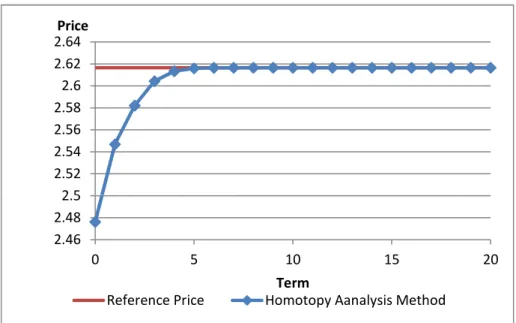
This section gives numerical examples to examine the efficiency of pricing options by the HAM. We compare our formula (11) with a reference price computed by analytical ex-pressions of Carr and Madan [4] for a European call. We use the following parameter set given in [10] : σ = 0.19071, κ = 0.49083, µ =−0.28113 and other parameters are set as S = 100,K = 100, r= 0.0549, q = 0.011, T = 0.1,α =−12.8. Figure 1 is the numerical result. The horizontal axis in the top figure represents the number of terms to approximate the infinite Taylor expansion in HAM and the vertical line represents option prices. The horizontal axis in the bottom figure represents the number of terms to approximate the infinite Taylor expansion in HAM and the vertical axis represents the difference between option price computed by HAM and the reference price. Both figures indicate that only the first five terms seem to give sufficient approximation.
The second case is down-and-out call price and we compare our formula with a refer-ence price computed by the finite differrefer-ence method [7] where the price at a grid point S = 100.01116 is chosen for comparison. For simplicity, the integral∫0T e−A1ω2τF[1
(b,∞)·
vSnc −1(x, τ)]dτ is approximated by the following simple trapezoid rule: T 2[F[1(b,∞)·v c Sn−1(x,0)] +e−A1ω 2T F[1(b,∞)·vSnc −1(x, T)]].
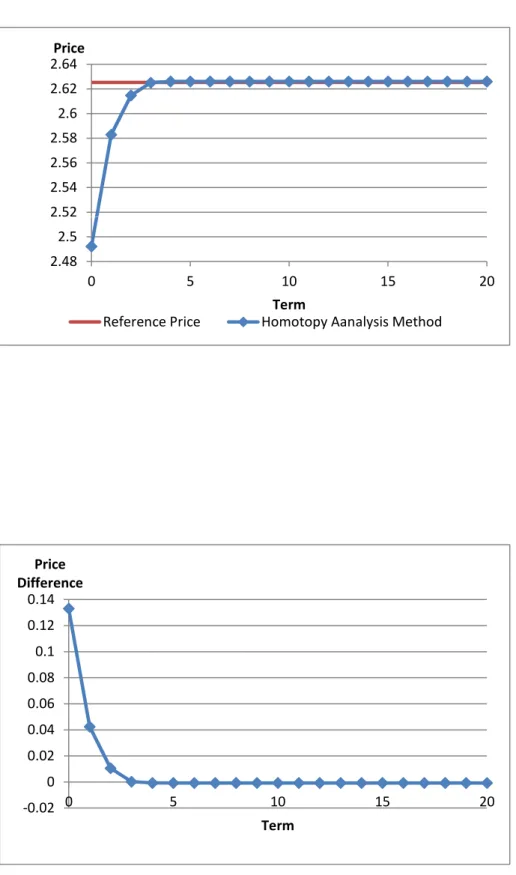
We use the same parameter set as that for the above example except α = −12.87 and B = 85 for the barrier. Figure 2 shows an numerical result. The horizontal axis in the top figure represents the number of terms to approximate the infinite Taylor expansion in HAM and the vertical axis represents option prices. The horizontal axis in the bottom figure represents the number of terms to approximate the infinite Taylor expansion in HAM and the vertical axis represents the difference between option price computed by HAM and the reference price. Similar to the case of European call option, both figures indicate that only the first five terms seem to provide a sufficient approximation. Therefore we conclude that Figure 1 and 2 demonstrate the efficiency of HAM in pricing these options.
7
Conclusion
In this paper, we present general methodology of applying the homotopy analysis method to European and barrier options under L´evy processes, and derive the sum of infinite series whose individual term may be calculated analytically. As an example of L´evy processes whose characteristic functions are available analytically, we used the Variance Gamma model. Our numerical examples demonstrates that HAM gives a sufficient approximation of original option price with the low orders of Taylor coefficients. Therefore HAM is efficient and applicable in practice. Moreover each term in the infinite series is expressed in terms of Fourier transform so the method of Fast Fourier transform can be used to achieve faster computation of each term. Once the price is computed, we can calculate option sensitivities such as delta and gamma easily as well. The method is easy to understand and can be applied to other type of options.
References
[1] S. Abbasbandy, The application of homotopy analysis method to solve a generalized Hirota-Satsuma coupled KdV equation,Physics Letters A 361 (2007) 478–483. [2] F. Black and M. Scholes, The pricing of options and corporate liabilities,The Journal
of Political Economy81(1973) 637–654.
[3] J. Cariboni and W. Schoutens, Pricing Credit Default Swaps under L´evy Models,
Journal of Computational Finance10(2007) 1–21.
[4] P. Carr and D. Madan, Option valuation using the fast Fourier transform,Journal of
Computational Finance2(1998) 61–73.
[5] R. Cont and P. Tankov, Financial modeling with jump processes(Chapman and Hall / CRC Press, London, 2004).
[6] L. Fen and V. Linetsky, Pricing discretely monitored barrier options and defaultable bonds in Levy process models: A Fast Hilbert transform approach, Mathematical
Finance18(2008) 337–384.
[7] F. Fiorani, Option pricing under the Variance Gamma Process (PhD thesis, Univer-sity of Trieste, 2004).
[8] L.C. Evans, Partial Differential Equations (American Mathematical Society, Provi-dence, 1998).
[9] M. Jeannin and M. Pistorius, A transform approach to calculate prices and greeks of barrier options driven by a class of Levy processes, Quantitative Finance10 (2010) 629–644.
[10] A. Hirsa and D. Madan, Pricing American options under variance Gamma, Journal
of Computational Finance7 (2004) 63–80.
[11] S. Liao, Numerically solving non-linear problems by the homotopy analysis method,
Computational Mechanics 20(1997) 530–540.
[12] D. Madan, P. Carr E. and Chang, The variance gamma process and option pricing,
European Finance Review2 (1998) 79–105.
[13] J.M. Ortega and W.C. Rheinboldt,Iterative solution of Nonlinear Equations in
[14] K. Sato,L´evy Processes and Infinitely Divisible Distributions (Cambridge University Press, Cambridge, 1999).
[15] J. Zhao and H.Y. Wong, A Closed-form Solution to American Options under General Diffusions,Quantitative Finance (2010) forthcoming.
[16] S. Zhu, An exact and explicit solution for the valuation of American put options,
2.5 2.52 2.54 2.56 2.58 2.6 2.62 2.64 Price 2.46 2.48 2.5 0 5 10 15 20 Term
Reference Price Homotopy Aanalysis Method
0.06 0.08 0.1 0.12 0.14 0.16 Price Difference 0 0.02 0.04 0.06 0 5 10 15 20 Term
2.52 2.54 2.56 2.58 2.6 2.62 2.64 Price 2.48 2.5 2.52 0 5 10 15 20 Term
Reference Price Homotopy Aanalysis Method
0.04 0.06 0.08 0.1 0.12 0.14 Price Difference -0.02 0 0.02 0.04 0 5 10 15 20 Term