SFB 649 Discussion Paper 2006-059
Discounted Optimal
Stopping for Maxima of
some Jump-Diffusion
Processes
Pavel V. Gapeev*
* Weierstrass Institute for Applied Analysis and Stochastics, Berlin, Germany
and
Russian Academy of Sciences, Institute of Control Sciences, Moscow, Russia
This research was supported by the Deutsche
Forschungsgemeinschaft through the SFB 649 "Economic Risk". http://sfb649.wiwi.hu-berlin.de ISSN 1860-5664 SFB 649, Humboldt-Universität zu Berlin
S
FB
6
4
9
E
C
O
N
O
M
I
C
R
I
S
K
B
E
R
L
I
N
Discounted optimal stopping for maxima
of some jump-diffusion processes
∗
Pavel V. Gapeev
We present solutions to some discounted optimal stopping problems for the maximum process in a model driven by a Brownian motion and a compound Poisson process with exponential jumps. The method of proof is based on reducing the initial problems to integro-differential free-boundary problems where the normal reflection and smooth fit may break down and the latter then be replaced by the continuous fit. The results can be interpreted as pricing perpetual American lookback options with fixed and floating strikes in a jump-diffusion model.
1. Introduction
The main aim of this paper is to present solutions to the discounted optimal stopping problems (2.4) and (5.1) for the maximum associated with the process X defined in (2.1) that solves the stochastic differential equation (2.2) driven by a Brownian motion and a compound Poisson process with exponentially distributed jumps. These problems are related to the option pricing theory in mathematical finance, where the process X can describe the price of a risky asset (e.g., a stock) on a financial market. In that case the values (2.4) and (5.1) can be formally interpreted asfair prices ofperpetual lookback options of American type withfixed and floating strikes in a jump-diffusion market model, respectively. For a continuous model the problems (2.4) and (5.1) were solved by Pedersen [21], Guo and Shepp [13], and Beibel and Lerche [4].
Observe that when K = 0 the problems (2.4) and (5.1) turn into the classical Russian option problem introduced and explicitly solved by Shepp and Shiryaev [30] by means of reducing the initial problem to an optimal stopping problem for a (continuous) two-dimensional Markov process and solving the latter problem using the smooth-fit and normal-reflection conditions. It was further observed in [31] that the change-of-measure theorem allows to reduce the Russian option problem to a one-dimensional optimal stopping problem that explained the simplicity of the solution in [30]. Building on the optimal stopping analysis of Shepp and Shiryaev [30]-[31], Duffie and Harrison [7] derived a rational economic value for the Russian option and
∗This research was supported by Deutsche Forschungsgemeinschaft through the SFB 649 Economic Risk. Mathematics Subject Classification 2000: Primary 60G40, 34K10, 91B70. Secondary 60J60, 60J75, 91B28.
Journal of Economic Literature Classification: G13.
Key words and phrases: Discounted optimal stopping problem, Brownian motion, compound Poisson pro-cess, maximum propro-cess, integro-differential free-boundary problem, continuous and smooth fit, normal reflection, a change-of-variable formula with local time on surfaces, perpetual lookback American options.
then extended their arbitrage arguments to perpetual lookback options. More recently, Shepp, Shiryaev and Sulem [32] proposed a barrier version of the Russian option where the decision about stopping should be taken before the price process reaches a ’dangerous’ positive level. Peskir [24] presented a solution to the Russian option problem in the finite horizon case (see also [8] for a numeric algorithm for solving the corresponding free-boundary problem and [10] for a study of asymptotic behavior of the optimal stopping boundary near expiration).
In the recent years, the Russian option problem in models with jumps was studied quite extensively. Gerber, Michaud and Shiu [12] and then Mordecki and Moreira [20] obtained closed form solutions to the perpetual Russian option problems for diffusions with negative exponential jumps. Asmussen, Avram and Pistorius [2] derived explicit expressions for the prices of perpetual Russian options in the dense class of L´evy processes with phase-type jumps in both directions by reducing the initial problem to the first passage time problem and solving the latter by martingale stopping and Wiener-Hopf factorization. Avram, Kyprianou and Pistorius [3] studied exit problems for spectrally negative L´evy processes and applied the results to solving optimal stopping problems associated with perpetual Russian and American put options.
In contrast to the Russian option problem, the problem (2.4) is necessarilytwo-dimensional
in the sense that it cannot be reduced to an optimal stopping problem for a one-dimensional (time-homogeneous) Markov process. Some other two-dimensional optimal stopping problems for continuous processes were earlier considered in [6] and [22]. The main feature of the optimal stopping problems for the maximum process in continuous models is that the normal-reflection condition at the diagonal holds and the optimal boundary can be characterized as a unique so-lution of a (first-order) nonlinear ordinary differential equation (see, e.g., [6], [30]-[31], [22], [21] and [13]). The key point in solving optimal stopping problems for jump processes established in [25]-[26] is that the smooth fit at the optimal boundary may break down and then be replaced by the continuous fit (see also [1] for necessary and sufficient conditions for the occurrence of smooth-fit condition and references to the related literature and [27] for an extensive overview). In the present paper we derive solutions to the problems (2.4) and (5.1) in a jump-diffusion model driven by a Brownian motion and a compound Poisson process with exponential jumps. Such model was considered in [18]-[19], [15]-[17] and [11] where the optimal stopping problems related to pricing American call and put options and convertible bonds were solved, respectively. We show that under some relationships on the parameters of the model the optimal stopping boundary can be uniquely determined as a component of a two-dimensional system of (first-order) nonlinear ordinary differential equations.
The paper is organized as follows. In Section 2, we formulate the optimal stopping problem for a two-dimensional Markov process related to the perpetual American fixed-strike lookback option problem and reduce it to an equivalent integro-differential free-boundary problem. In Section 3, we present a solution to the free-boundary problem and derive (first-order) nonlinear ordinary differential equations for the optimal stopping boundary under different relationships on the parameters of the model as well as specify the asymptotic behavior of the boundary. In Section 4, we verify that the solution of the free-boundary problem turns out to be a solution of the initial optimal stopping problem. In Section 5, we give some concluding remarks as well as present an explicit solutionto the optimal stopping problem related to the perpetual American
floating-strikelookback option problem. The main results of the paper are stated in Theorems 4.1 and 5.1.
2. Formulation of the problem
In this section we introduce the setting and notation of the two-dimensional optimal stopping problem which is related to the perpetual American fixed-strike lookback option problem and formulate an equivalent integro-differential free-boundary problem.
2.1. For a precise formulation of the problem let us consider a probability space (Ω,F, P) with a standard Brownian motion B = (Bt)t≥0 and a jump process J = (Jt)t≥0 defined by
Jt = PNi=1t Yi, where N = (Nt)t≥0 is a Poisson process of the intensity λ and (Yi)i∈N is a
sequence of independent random variables exponentially distributed with parameter 1 (B, N
and (Yi)i∈N are supposed to be independent). Assume that there exists a process X = (Xt)t≥0 given by: Xt=x exp r−σ2/2−λθ/(1−θ)t+σ Bt+θ Jt (2.1) and hence solving the stochastic differential equation:
dXt=rXt−dt+σXt−dBt+Xt−
Z ∞
0
eθy−1(µ(dt, dy)−ν(dt, dy)) (X0 =x) (2.2) where µ(dt, dy) is the measure of jumps of the process J with the compensator ν(dt, dy) =
λdtI(y > 0)e−ydy, and x > 0 is given and fixed. It can be assumed that the process X
describes a stock price on a financial market, where r >0 is the interest rate, and σ ≥0 and
θ < 1, θ 6= 0, are the volatilities of continuous and jump part, respectively. Note that the assumption θ < 1 guarantees that the jumps of X are integrable and that is not a restriction. With the process X let us associate the maximum process S = (St)t≥0 defined by:
St = max 0≤u≤tXu ∨s (2.3)
for an arbitrary s ≥ x > 0. The main purpose of the present paper is to derive a solution to the optimal stopping problem for the time-homogeneous (strong) Markov process (X, S) = (Xt, St)t≥0 given by: V∗(x, s) = sup τ Ex,s e−(r+δ)τ(Sτ −K)+ (2.4) where the supremum is taken over all stopping times τ of the process X (i.e., stopping times with respect to the natural filtration of X), and Px,s is a probability measure under which
the (two-dimensional) process (X, S) defined in (2.1)-(2.3) starts at (x, s) ∈ E. Here by
E = {(x, s) | 0 < x ≤ s} we denote the state space of the process (X, S). The value (2.4) coincides with an arbitrage-free priceof a fixed-strike lookback American option with the strike price K >0 and the discounting rate δ >0 (see, e.g., [34]). Note that in the continuous case
σ > 0 and θ = 0 the problem (2.4) was solved in [21] and [13]. It is also seen that if σ = 0 and 0 < θ <1 with r−λθ/(1−θ)≥0, then the optimal stopping time in (2.4) is infinite.
2.2. Let us first determine the structure of the optimal stopping time in the problem (2.4). Applying the arguments from [6; Subsection 3.2] and [22; Proposition 2.1] to the optimal stopping problem (2.4) we see that it is never optimal to stop when Xt = St for t ≥ 0 (this
fact will be also proved independently below). It follows directly from the structure of (2.4) that it is never optimal to stop when St ≤ K for t ≥ 0. In other words, this shows that all
points (x, s) from the set:
C0 ={(x, s)∈E |0< x≤s≤K} (2.5)
and from the diagonal {(x, s)∈E |x=s} belong to the continuation region:
C∗ ={(x, s)∈E |V∗(x, s)>(s−K)+}. (2.6) Let us fix (x, s) ∈ C∗ and let τ∗ = τ∗(x, s) denote the optimal stopping time in (2.4). Then, taking some point (y, s) such that 0 < y ≤ s, by virtue of the structure of optimal stopping problem (2.4) and (2.3) with (2.1) we get:
V∗(y, s)≥Ey,s e−λτ∗(S τ∗ −K) + ≥Ex,s e−λτ∗(S τ∗−K) + =V∗(x, s)>(s−K)+. (2.7) These arguments together with the comments in [6; Subsection 3.3] and [22; Subsection 3.3] as well as the assumption that V∗(x, s) is continuous show that there exists a function g∗(s) for
s > K such that the continuation region (2.6) is an open set consisting of (2.5) and of the set:
C∗00={(x, s)∈E |g∗(s)< x≤s, s > K} (2.8)
while the stopping region is the closure of the set:
D∗ ={(x, s)∈E |0< x < g∗(s), s > K}. (2.9)
Let us now show that in (2.8)-(2.9) the function g∗(s) is increasing on (K,∞) (this fact will be also proved independently below). Since in (2.4) the function s−K is linear in s on (K,∞), by means of standard arguments it is shown that V∗(x, s)− (s −K) is decreasing in s on (K,∞). Hence, if for given (x, s) ∈ C∗00 we take s0 such that K < s0 < s, then
V∗(x, s0)−(s0−K)≥V∗(x, s)−(s−K)>0 so that (x, s0)∈C∗00, and thus the desired assertion follows.
Let us denote by W∗(x, s) and a∗s the value function and the boundary of the optimal stopping problem related to the Russian option problem. It is easily seen that in case K = 0 the function W∗(x, s) coincides with (2.4) and (5.1), while under different relationships on the parameters of the model a∗ < 1 can be uniquely determined by (5.11), (5.13), (5.15) and (5.17), respectively. Suppose that g∗(s)> a∗s for some s > K. Then for any x∈ (a∗s, g∗(s)) given and fixed we have W∗(x, s)−K > s−K =V∗(x, s) contradicting the obvious fact that
W∗(x, s)−K ≤ V∗(x, s) for all (x, s) ∈ E with s > K as it is clearly seen from (2.4). Thus, we may conclude that g∗(s)≤a∗s < s for all s > K.
2.3. Standard arguments imply that in this case the infinitesimal operator L of the process (X, S) acts on a function F ∈C2,1(E) (or F ∈C1,1(E) when σ= 0) according to the rule:
(LF)(x, s) = (r+ζ)x Fx(x, s)+ σ2 2 x 2 Fxx(x, s)+ Z ∞ 0
F xeθy, xeθy∨s−F(x, s)λe−ydy (2.10) for all 0 < x < s with ζ = −λθ/(1−θ). Using standard arguments based on the strong Markov property it follows that V∗ ∈ C2,1(C∗ ≡ C0 ∪C∗00) (or V∗ ∈ C1,1(C∗ ≡ C0∪C∗00) when
(2.4) and the unknown boundary g∗(s) from (2.8)-(2.9) using the results of general theory of optimal stopping problems for Markov processes (see, e.g., [33; Chapter III, Section 8]) we can formulate the following integro-differential free-boundary problem:
(LV)(x, s) = (r+δ)V(x, s) for (x, s)∈C≡C0∪C00 (2.11)
V(x, s)
x=g(s)+=s−K (continuous fit) (2.12)
V(x, s) = (s−K)+ for (x, s)∈D (2.13)
V(x, s)>(s−K)+ for (x, s)∈C (2.14) where C00 and D are defined as C∗00 and D∗ in (2.8) and (2.9) with g(s) instead of g∗(s), respectively, and (2.12) playing the role of instantaneous-stopping condition is satisfied for all
s > K. Observe that the superharmonic characterization of the value function (see [9] and
[33]) implies that V∗(x, s) is the smallest function satisfying (2.11)-(2.13) with the boundary
g∗(s). Moreover, under some relationships on the parameters of the model which are specified below, the following conditions can be satisfied or break down:
Vx(x, s) x=g(s)+= 0 (smooth fit) (2.15) Vs(x, s) x=s− = 0 (normal reflection) (2.16) for all s > K. Note that in the case σ > 0 and θ= 0 the free-boundary problem (2.11)-(2.16) was solved in [21] and [13].
2.4. In order to specify the boundary g∗(s) as a solution of the free-boundary problem (2.11)-(2.14) and (2.15)-(2.16), for further considerations we need to observe that from (2.4) it follows that the inequalities:
0≤sup τ Ex,s e−(r+δ)τSτ −K ≤sup τ Ex,s e−(r+δ)τ(Sτ −K)+ ≤sup τ Ex,s e−(r+δ)τSτ (2.17) which are equivalent to:
0≤W∗(x, s)−K ≤V∗(x, s)≤W∗(x, s) (2.18) hold for all (x, s)∈E with s > K. Thus, setting x=s in (2.18) we get:
0≤ W∗(s, s) s − K s ≤ V∗(s, s) s ≤ W∗(s, s) s (2.19)
for all s > K so that letting s go to infinity in (2.19) we obtain: lim inf s→∞ V∗(s, s) s = lim sups→∞ V∗(s, s) s = lims→∞ W∗(s, s) s . (2.20)
3
Solution of the free-boundary problem
In this section we obtain solutions to the free-boundary problem (2.11)-(2.16) and derive ordinary differential equations for the optimal boundary under different relationships on the parameters of the model (2.1)-(2.2).
3.1. By means of straightforward calculations we reduce equation (2.11) to the form: (r+ζ)x Vx(x, s) + σ2 2 x 2V xx(x, s)−αλxαG(x, s) = (r+δ+λ)V(x, s) (3.1)
with α = 1/θ and ζ =−λθ/(1−θ), where taking into account conditions (2.12)-(2.13) we set:
G(x, s) =− Z s x V(z, s) dz zα+1 − Z ∞ s V(z, z) dz zα+1 if α= 1/θ >1 (3.2) G(x, s) = Z x g(s) V(z, s) dz zα+1 − s−K αg(s)α if α = 1/θ <0 (3.3)
for all 0 < x < g(s) and s > K. Then from (3.1) and (3.2)-(3.3) it follows that the function
G(x, s) solves the following (third-order) ordinary differential equation:
σ2 2 x 3G xxx(x, s) + σ2(α+ 1) +r+ζx2Gxx(x, s) (3.4) + (α+ 1) σ2α 2 +r+ζ −(r+δ+λ) x Gx(x, s)−αλ G(x, s) = 0
for 0< x < g(s) and s > K, which has the following general solution:
G(x, s) =C1(s) xβ1 β1 +C2(s) xβ2 β2 +C3(s) xβ3 β3 (3.5) where C1(s), C2(s) and C3(s) are some arbitrary functions and β3 < β2 < β1 are the real roots of the corresponding (characteristic) equation:
σ2 2 β 3+ σ2 α− 1 2 +r+ζ β2+ α σ2(α−1) 2 +r+ζ −(r+δ+λ) β−αλ= 0. (3.6) Therefore, differentiating both sides of the formulas (3.2)-(3.3) we get that the integro-differential equation (3.1) has the general solution:
V(x, s) = C1(s)xγ1 +C2(s)xγ2 +C3(s)xγ3 (3.7) where we set γi = βi +α for i = 1,2,3. Further we assume that the functions C1(s), C2(s) and C3(s) as well as the boundary g(s) are continuously differentiable for s > K. Observe that if σ= 0 and r+ζ <0 then it is seen that (3.4) degenerates into a second-order ordinary differential equation, and in that case we can set C3(s) ≡ 0 in (3.5) as well as in (3.7), while the roots of equation (3.6) are explicitly given by:
βi = r+δ+λ 2(r+ζ) − α 2 −(−1) i s r+δ+λ 2(r+ζ) − α 2 2 + αλ r+ζ (3.8) for i= 1,2.
3.2. Let us first determine the boundary g∗(s) for the case σ >0 and α= 1/θ < 0. Then we have β3 <0< β2 <−α <1−α < β1 so that γ3 < α < γ2 <0<1< γ1 with γi =βi+α,
where βi fori= 1,2,3 are the roots of equation (3.6). Since in this case the process X can leave
the part of continuation region g∗(s) < x ≤ s and hits the diagonal {(x, s)∈ E|x =s} only continuously, we may assume that both the smooth-fit and normal-reflection conditions (2.15) and (2.16) are satisfied. Hence, applying conditions (3.3), (2.12) and (2.15) to the functions (3.5) and (3.7), we get that the following equalities hold:
C1(s) g(s)γ1 β1 +C2(s) g(s)γ2 β2 +C3(s) g(s)γ3 β3 =−s−K α (3.9) C1(s)g(s)γ1 +C2(s)g(s)γ2 +C3(s)g(s)γ3 =s−K (3.10) γ1C1(s)g(s)γ1 +γ2C2(s)g(s)γ2 +γ3C3(s)g(s)γ3 = 0 (3.11) for s > K. Thus, by means of straightforward calculations, from (3.9)-(3.11) we obtain that the solution of system (2.11)-(2.13)+(2.15) takes the form:
V(x, s;g(s)) (3.12) = β1γ2γ3(s−K)/α (γ2 −γ1)(γ1 −γ3) x g(s) γ1 + β2γ1γ3(s−K)/α (γ2−γ1)(γ3−γ2) x g(s) γ2 + β3γ1γ2(s−K)/α (γ1−γ3)(γ3−γ2) x g(s) γ3
for 0< x < g(s) and s > K. Then applying condition (2.16) to the function (3.7) we get:
C10(s)sγ1 +C0
2(s)s
γ2 +C0
3(s)s
γ3 = 0 (3.13)
from where using the solution of system (3.9)-(3.11) it follows that the function g(s) solves the following (first-order) ordinary differential equation:
g0(s) = g(s) γ1γ2γ3(s−K) (3.14) ×β1γ2γ3(γ2−γ3)(s/g(s)) γ1 −β 2γ1γ3(γ1−γ3)(s/g(s))γ2 +β3γ1γ2(γ1 −γ2)(s/g(s))γ3 β1(γ2−γ3)(s/g(s))γ1 −β2(γ1−γ3)(s/g(s))γ2 +β3(γ1−γ2)(s/g(s))γ3
for s > K with γi =βi+α, where βi for i= 1,2,3 are the roots of equation (3.6). By means
of standard arguments it can be shown that the right-hand side of equation (3.14) is positive so that the function g(s) is strictly increasing on (K,∞).
Let us denote h∗(s) = g∗(s)/s for all s > K and set h = lim sups→∞h∗(s) and h = lim infs→∞h∗(s). In order to specify the solution of equation (3.14) which coincides with the optimal stopping boundary g∗(s), we observe that from the expression (3.12) it follows that (2.20) directly implies: β1γ2γ3(γ3−γ2)h−γ1 +β2γ1γ3(γ1−γ3)h −γ2 +β3γ1γ2(γ2−γ1)h −γ3 (3.15) =β1γ2γ3(γ3−γ2)h −γ1 +β2γ1γ3(γ1−γ3)h−γ2 +β3γ1γ2(γ2−γ1)h−γ3 =β1γ2γ3(γ3−γ2)a−∗γ1+β2γ1γ3(γ1 −γ3)a−∗γ2 +β3γ1γ2(γ2−γ1)a−∗γ3
where a∗ is uniquely determined by (5.11) under K = 0. Then, using the fact that h∗(s) =
g∗(s)/s≤a∗ for s > K and thus h≤h≤a∗ <1, from (3.15) we get that h=h=a∗. Hence, we obtain that the optimal boundary g∗(s) should satisfy the property:
lim
s→∞
g∗(s)
which gives a condition on the infinity for the equation (3.14). By virtue of the results on the existence and uniqueness of solutions for first-order ordinary differential equations, we may therefore conclude that condition (3.16) uniquely specifies the solution of equation (3.14) that corresponds to the problem (2.4). Taking into account the expression (3.12), we also note that from inequalities (2.18) it follows that the optimal boundary g∗(s) satisfies the properties:
g∗(K+) = 0 and g∗(s)∼A∗(s−K)1/γ1 under s↓K (3.17) for some constant A∗ >0 which can be also determined by means of condition (3.16) above.
3.3. Let us now determine the boundary g∗(s) for the case σ = 0 and α = 1/θ < 0. Then we have 0< β2 <−α <1−α < β1 so that α < γ2 <0<1< γ1 with γi =βi+α, where βi for
i = 1,2 are given by (3.6). In this case, applying conditions (3.3) and (2.12) to the functions (3.5) and (3.7) with C3(s)≡0, we get that the following equalities hold:
C1(s) g(s)γ1 β1 +C2(s) g(s)γ2 β2 =−s−K α (3.18) C1(s)g(s)γ1+C2(s)g(s)γ2 =s−K (3.19) for s > K. Thus, by means of straightforward calculations, from (3.18)-(3.19) we obtain that the solution of system (2.11)-(2.13) takes the form:
V(x, s;g(s)) = β1γ2(s−K) α(γ1−γ2) x g(s) γ1 − β2γ1(s−K) α(γ1−γ2) x g(s) γ2 (3.20) for 0 < x < g(s) and s > K. Since in this case r+ζ > 0 so that the process X hits the diagonal {(x, s) ∈ E|x = s} only continuously, we may assume that the normal-reflection condition (2.16) holds. Hence, applying condition (2.16) to the function (3.7) with C3(s)≡0, we get:
C10(s)sγ1 +C0
2(s)s
γ2 = 0 (3.21)
from where using the solution of system (3.18)-(3.19) it follows that the function g(s) solves the differential equation:
g0(s) = g(s)
γ1γ2(s−K)
β1γ2(s/g(s))γ1 −β2γ1(s/g(s))γ2
β1(s/g(s))γ1 −β2(s/g(s))γ2
(3.22) for s > K with γi =βi +α, where βi for i = 1,2 are given by (3.8). By means of standard
arguments it can be shown that the right-hand side of equation (3.22) is positive so that the function g(s) is strictly increasing on (K,∞). Note that in this case the smooth-fit condition (2.15) fails to hold, that can be explained by the fact that leaving the part of continuation region g∗(s) < x ≤ s the process X can pass through the boundary g∗(s) only by jumping. Such an effect was earlier observed in [25]-[26] by solving some other optimal stopping problems for jump processes. According to the results in [1] we may conclude that this property appears because of finite intensity of jumps and exponential distribution of jump sizes of the compound Poisson process J.
Let us recall that h = lim sups→∞h∗(s) and h = lim infs→∞h∗(s) with h∗(s) = g∗(s)/s for all s > K. In order to specify the solution of equation (3.22) which coincides with the
optimal stopping boundary g∗(s), we observe that from the expression (3.20) it follows that (2.20) directly implies: β1γ2h −γ1 −β2γ1h−γ2 =β1γ2h−γ1 −β2γ1h −γ2 =β1γ2a−∗γ1 −β2γ1a−∗γ2 (3.23) where a∗ is uniquely determined by (5.13) under K = 0. Then, using the fact that h∗(s) =
g∗(s)/s≤a∗ for s > K and thus h≤h≤a∗ <1, from (3.23) we get that h=h=a∗. Hence, we obtain that the optimal boundary g∗(s) should satisfy the property (3.16) which gives a condition on the infinity for the equation (3.22). By virtue of the results on the existence and uniqueness of solutions for first-order ordinary differential equations, we may therefore conclude that condition (3.16) uniquely specifies the solution of equation (3.22) that corresponds to the problem (2.4). Taking into account the expression (3.20), we also note that from inequalities (2.18) it follows that the optimal boundary g∗(s) satisfies the properties (3.17) for some constant
A∗ >0 which can be also determined by means of condition (3.16) above.
3.4. Let us now determine the optimal boundary g∗(s) for the case σ >0 and α= 1/θ >1. Then we have β3 < −α < 1−α < β2 < 0 < β1 so that γ3 < 0 < 1 < γ2 < α < γ1 with
γi = βi +α, where βi for i = 1,2,3 are the roots of equation (3.6). By virtue of the same
arguments as mentioned above, in this case we may also assume that both the smooth-fit and normal-reflection conditions (2.15) and (2.16) hold. Hence, applying conditions (3.3), (2.12) and (2.15) to the functions (3.5) and (3.7), respectively, we get that the following equalities hold: C1(s) sγ1 β1 +C2(s) sγ2 β2 +C3(s) sγ3 β3 =f(s)sα(s−K) (3.24) C1(s)g(s)γ1 +C2(s)g(s)γ2 +C3(s)g(s)γ3 =s−K (3.25) γ1C1(s)g(s)γ1 +γ2C2(s)g(s)γ2 +γ3C3(s)g(s)γ3 = 0 (3.26) where we set: f(s) = − 1 s−K Z ∞ s V(z, z) dz zα+1 (3.27)
for s > K. Thus, by means of straightforward calculations, from (3.24)-(3.26) we obtain that the solution of system (2.11)-(2.13)+(2.15) takes the form:
V(x, s;g(s)) (3.28) = β1(s−K)[β2β3(γ2−γ3)s αf(s) +β 3γ3(s/g(s))γ2 −β2γ2(s/g(s))γ3] β2β3(γ2−γ3)(s/g(s))γ1 −β1β3(γ1−γ3)(s/g(s))γ2 +β1β2(γ1−γ2)(s/g(s))γ3 x g(s) γ1 + β2(s−K)[β1β3(γ3−γ1)s αf(s)−β 3γ3(s/g(s))γ1 +β1γ1(s/g(s))γ3] β2β3(γ2−γ3)(s/g(s))γ1 −β1β3(γ1−γ3)(s/g(s))γ2 +β1β2(γ1−γ2)(s/g(s))γ3 x g(s) γ2 + β3(s−K)[β1β2(γ1−γ2)s αf(s) +β 2γ2(s/g(s))γ1 −β1γ1(s/g(s))γ2] β2β3(γ2−γ3)(s/g(s))γ1 −β1β3(γ1−γ3)(s/g(s))γ2 +β1β2(γ1−γ2)(s/g(s))γ3 x g(s) γ3
for 0 < x < g(s) and s > K. Inserting the expressions (3.5) and (3.7) into the formula (3.2), letting x=s and differentiating the both sides of the obtained equality, we get:
C10(s)s γ1 β1 +C20(s)s γ2 β2 +C30(s)s γ3 β3 = 0 (3.29)
from where using the solution of system (3.24)-(3.26) it follows that the function f(s) solves the differential equation:
f0(s) =− f(s) s−K (3.30) + β1β2β3f(s)[(γ2−γ3)(s/g(s)) γ1 −(γ 1−γ3)(s/g(s))γ2 + (γ1−γ2)(s/g(s))γ3] s[β2β3(γ2−γ3)(s/g(s))γ1−β1β3(γ1−γ3)(s/g(s))γ2 +β1β2(γ1−γ2)(s/g(s))γ3] +β3γ3(γ1−γ2)(s/g(s)) γ1+γ2 −β 2γ2(γ1−γ3)(s/g(s))γ1+γ3 +β1γ1(γ2−γ3)(s/g(s))γ2+γ3 sα+1[β 2β3(γ2−γ3)(s/g(s))γ1 −β1β3(γ1−γ3)(s/g(s))γ2 +β1β2(γ1−γ2)(s/g(s))γ3] for s > K. Applying the condition (2.16) to the function (3.7), we get that the equality (3.13) holds, from where it follows that the function g(s) solves the differential equation:
g0(s) = g(s) s−K (3.31) ×β3γ3(γ1−γ2)(s/g(s)) γ1+γ2−β 2γ2(γ1−γ3)(s/g(s))γ1+γ3+β1γ1(γ2−γ3)(s/g(s))γ2+γ3 β3(γ1−γ2)(s/g(s))γ1+γ2 −β2(γ1 −γ3)(s/g(s))γ1+γ3 +β1(γ2−γ3)(s/g(s))γ2+γ3 × β2β3(γ2−γ3)(s/g(s)) γ1 −β 1β3(γ1−γ3)(s/g(s))γ2 +β1β2(γ1−γ2)(s/g(s))γ3 η2η3(γ2−γ3)(s/g(s))γ1 −η1η3(γ1−γ3)(s/g(s))γ2 +η1η2(γ1−γ2)(s/g(s))γ3 −ρf(s)sα for s > K with ηi =βiγi for i= 1,2,3, and ρ=β1β2β3(γ1−γ2)(γ1−γ3)(γ2−γ3).
In order to specify the solution of equation (3.30) let us define the function:
f∗(s) = − 1 s−K Z ∞ s V∗(z, z) dz zα+1 (3.32)
for all s > K. Then by virtue of the inequalities (2.18), using the expression (5.14) we obtain the function (3.32) is well-defined and should satisfy the property:
lim s→∞f∗(s)s α =γ 2(γ3−1)/[(γ2−γ1)(β1(γ3−1)aγ∗1 −β3(γ1−1)aγ∗3)] (3.33) +γ3(γ1−1)/[(γ3−γ2)(β2(γ1−1)aγ∗2 −β1(γ2−1)aγ∗1)] +γ1(γ2−1)/[(γ1−γ3)(β3(γ2−1)aγ∗3 −β2(γ3−1)aγ∗2)]
where a∗ is uniquely determined by (5.15) under K = 0. From (3.27) and (3.32) it therefore follows that (3.33) gives a condition on the infinity for the equation (3.30).
Let us recall that h = lim sups→∞h∗(s) and h= lim infs→∞h∗(s) with h∗(s) = g∗(s)/s for all s > K. In order to specify the solution of equation (3.31) which coincides with the optimal stopping boundary g∗(s), we observe that from the expressions (3.28) and (3.33) it follows that (2.20) directly implies: (γ2−γ3)h −γ1 + (γ3−γ1)h−γ2+ (γ1−γ2)h−γ3 β2β3(γ2−γ3)h−γ1 −β1β3(γ1−γ3)h−γ2 +β1β2(γ1−γ2)h−γ3 (3.34) = (γ2 −γ3)h −γ1 + (γ 3−γ1)h −γ2 + (γ1−γ2)h −γ3 β2β3(γ2−γ3)h −γ1 −β1β3(γ1−γ3)h −γ2 +β1β2(γ1−γ2)h −γ3 = (γ2 −γ3)a −γ1 ∗ + (γ3−γ1)a∗−γ2 + (γ1−γ2)a−∗γ3 β2β3(γ2−γ3)a −γ1 ∗ −β1β3(γ1−γ3)a −γ2 ∗ +β1β2(γ1−γ2)a −γ3 ∗ .
Then, using the fact that h∗(s) =g∗(s)/s≤a∗ for s > K and thush≤h≤a∗ <1, from (3.34) we get that h = h = a∗. Hence, we obtain that the optimal boundary g∗(s) should satisfy the property (3.16) which gives a condition on the infinity for the equation (3.31). By virtue of the results on the existence and uniqueness of solutions for systems of first-order ordinary differential equations, we may therefore conclude that conditions (3.33) and (3.16) uniquely specifies the solution of system (3.30)+(3.31) that corresponds to the problem (2.4). Taking into account the expression (3.28), we also note that from inequalities (2.18) it follows that the optimal boundary g∗(s) satisfies the properties (3.17) for some constant A∗ >0 which can be also determined by means of the condition (3.16) above.
3.5. Let us finally determine the boundary g∗(s) for the case σ = 0 and α= 1/θ >1 with
r+ζ =r−λθ/(1−θ)<0. Then we have β2 <−α <1−α < β1 <0 so that γ2 <0<1< γ1 with γi = βi +α, where βi for i = 1,2 are given by (3.6). Since in this case the process X
can leave the continuation region g∗(s) < x ≤ s only continuously, we may assume that the smooth-fit condition (2.15) holds. Hence, applying conditions (2.12) and (2.15) to the function (3.7), we get that the following equalities hold:
C1(s)g(s)γ1 +C2(s)g(s)γ2 =s−K (3.35)
γ1C1(s)g(s)γ1 +γ2C2(s)g(s)γ2 = 0 (3.36) for s > K. Thus, by means of straightforward calculations, from (3.35)-(3.36) we obtain that the solution of system (2.11)-(2.13)+(2.15) takes the form:
V(x, s;g(s)) = γ2(s−K) γ2−γ1 x g(s) γ1 − γ1(s−K) γ2−γ1 x g(s) γ2 (3.37) for 0< x < g(s) and s > K. Inserting the expressions (3.5) and (3.7) with C3(s)≡0 into the formula (3.2), letting x=s and differentiating the both sides of the obtained equality, we get:
C10(s)s γ1 β1 +C20(s)s γ2 β2 = 0 (3.38)
from where using the solution of system (3.35)-(3.36) it follows that the function g(s) satisfies the differential equation:
g0(s) = g(s)
γ1γ2(s−K)
β2γ2(s/g(s))γ1 −β1γ1(s/g(s))γ2
β2(s/g(s))γ1 −β1(s/g(s))γ2
(3.39) for s > K with γi =βi +α, where βi for i = 1,2 are given by (3.8). By means of standard
arguments it can be shown that the right-hand side of equation (3.39) is positive so that the function g(s) is strictly increasing on (K,∞). Note that in this case the normal-reflection condition (2.16) fails to hold, that can be explained by the fact that the process X can hit the diagonal {(x, s)∈E|x=s} only by jumping.
Let us recall that h = lim sups→∞h∗(s) and h = lim infs→∞h∗(s) with h∗(s) = g∗(s)/s for all s > K. In order to specify the solution of equation (3.39) which coincides with the optimal stopping boundary g∗(s), we observe that from the expression (3.37) it follows that (2.20) directly implies: γ2h −γ1 −γ1h −γ2 =γ 2h −γ1 −γ 1h −γ2 =γ2a−∗γ1 −γ1a−∗γ2 (3.40)
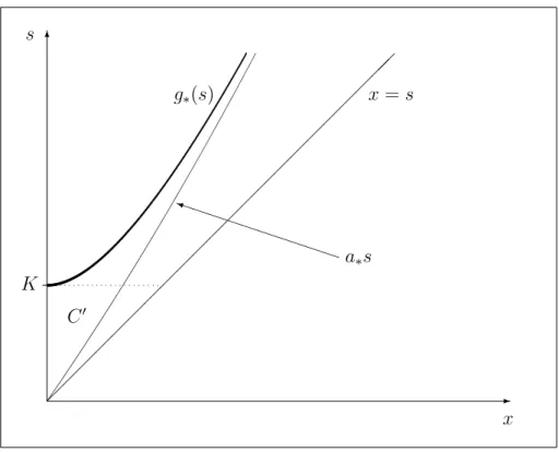
-6 P P P P P P P P P P i K s x g∗(s) x=s a∗s C0
Figure 1. A computer drawing of the optimal stopping boundary g∗(s) .
where a∗ is uniquely determined by (5.17) under K = 0. Then, using the fact that h∗(s) =
g∗(s)/s≤a∗ for s > K and thus h≤h≤a∗ <1, from (3.40) we get that h=h=a∗. Hence, we obtain that the optimal boundary g∗(s) should satisfy the property (3.16) which gives a condition on the infinity for the equation (3.39). By virtue of the results on the existence and uniqueness of solutions for first-order ordinary differential equations, we may therefore conclude that condition (3.16) uniquely specifies the solution of equation (3.39) that corresponds to the problem (2.4). Taking into account the expression (3.37), we also note that from inequalities (2.18) it follows that the optimal boundary g∗(s) satisfies the properties (3.17) for some constant
A∗ >0 which can be also determined by means of the condition (3.16) above.
3.6. Observe that the arguments above show that if we start at the point (x, s)∈C0 then it is easily seen that the process (X, S) can be stopped optimally after it passes through the point (K, K). Thus, using standard arguments based on the strong Markov property it follows that:
V∗(x, s) = U(x;K)V∗(K, K) (3.41) for all (x, s)∈C0 with V∗(K, K) = lims↓KV∗(K, s), where we set:
U(x;K) =Ex
e−(r+δ)σ∗ (3.42)
and
σ∗ = inf{t ≥0|Xt≥K}. (3.43)
By means of straightforward calculations based on solving the corresponding boundary value problem (see also [2]-[3] and [17]) it follows that when α = 1/θ <0 holds, we have:
U(x;K) = x
K
γ1
(3.44) with γ1 =β1+α, where if σ >0 then β1 is the largest root of equation (3.6), while if σ = 0 then β1 is given by (3.8). It also follows that when α= 1/θ >1 holds, then we have:
U(x;K) = β1γ2 α(γ1−γ2) x K γ1 − β2γ1 α(γ1−γ2) x K γ2 (3.45) with γi = βi +α, where if σ > 0 then βi for i = 1,2 are the two largest roots of equation
(3.6), while if σ= 0 and r+ζ =r−λθ/(1−θ)<0 then βi for i= 1,2 are given by (3.8).
4. Main result and proof
In this section using the facts proved above we formulate and prove the main result of the paper.
Theorem 4.1. Let the process (X, S) be defined in (2.1)-(2.3). Then the value function of the problem (2.4) takes the expression:
V∗(x, s) = V(x, s;g∗(s)), if g∗(s)< x < s and s > K U(x;K)V∗(K, K), if 0< x≤s ≤K s−K, if 0< x≤g∗(s) and s > K (4.1)
[with V∗(K, K) = lims↓KV∗(K, s)] and the optimal stopping time is explicitly given by:
τ∗ = inf{t≥0|Xt ≤g∗(St)} (4.2)
where the functions V(x, s;g(s)) and U(x;K) as well as the increasing boundary g∗(s)≤a∗s <
s for s > K satisfying g∗(K+) = 0 and g∗(s) ∼ A∗(s −K)1/γ under s ↓ K [see Figure 1
above] are specified as follows:
(i): if σ > 0 and θ < 0 then V(x, s;g(s)) is given by (3.12), U(x;K) is given by (3.44), and g∗(s) is uniquely determined from the differential equation (3.14) and the condition (3.16),
where γi = βi + 1/θ and βi for i = 1,2,3 are the roots of equation (3.6), while a∗ is found
from equation (5.11) under K = 0;
(ii): if σ = 0 and θ <0 then V(x, s;g(s)) is given by (3.20), U(x;K) is given by (3.44), and g∗(s) is uniquely determined from the differential equation (3.22) and the condition (3.16),
where γi = βi + 1/θ and βi for i = 1,2 are given by (3.8), while a∗ is found from equation
(5.13) under K = 0;
(iii): if σ > 0 and 0 < θ < 1 then V(x, s;g(s)) is given by (3.28), U(x;K) is given by (3.45), and g∗(s) is uniquely determined from the system of differential equations (3.30)+(3.31) and the conditions (3.33)+(3.16), where γi =βi + 1/θ and βi for i = 1,2,3 are the roots of
(iv): if σ = 0 and 0< θ <1 with r−λθ/(1−θ)<0 then V(x, s;g(s)) is given by (3.37),
U(x;K) is given by (3.45), and g∗(s) is uniquely determined from the differential equation
(3.39) and the condition (3.16), where γi = βi+ 1/θ and βi for i = 1,2 are given by (3.8),
while a∗ is found from equation (5.17) under K = 0.
Proof. In order to verify the assertions stated above, it remains us to show that the function (4.1) coincides with the value function (2.4) and the stopping time τ∗ from (4.2) with the boundary g∗(s) specified above is optimal. For this, let us denote by V(x, s) the right-hand side of the expression (4.1). In this case, by means of straightforward calculations and the assumptions above it follows that the function V(x, s) solves the system (2.11)-(2.13), and condition (2.15) is satisfied when either σ > 0 or r−λθ/(1−θ) < 0 holds, while condition (2.16) is satisfied when either σ > 0 or θ < 0 holds. Then taking into account the fact that the boundary g∗(s) is assumed to be continuously differentiable for s > K and applying the change-of-variable formula from [23; Theorem 3.1] to e−(r+δ)tV(Xt, St), we obtain:
e−(r+δ)tV(Xt, St) = V(x, s) + Z t 0 e−(r+δ)u(LV −(r+δ)V)(Xu, Su)I(Xu 6=g∗(Su))du (4.3) + Z t 0 e−(r+δ)uVs(Xu−, Su−)dSu− X 0<u≤t e−(r+δ)uVs(Xu−, Su−) ∆Su+Mt
where the process (Mt)t≥0 defined by:
Mt = Z t 0 e−(r+δ)uVx(Xu−, Su−)σXu−dBu (4.4) + Z t 0 Z ∞ 0 e−(r+δ)uV Xu−eθy, Xu−eθy∨Su− −V(Xu−, Su−) (µ(du, dy)−ν(du, dy)) is a local martingale under Px,s. Observe that when either σ >0 or 0< θ <1, the time spent
by the process X at the diagonal {(x, s) ∈ E | 0 < x≤ s} is of Lebesgue measure zero that allows to extend (LV −(r+δ)V)(x, s) arbitrarily to x=s. When either σ > 0 or θ < 0, the time spent by the process X at the boundary g∗(S) is of Lebesgue measure zero that allows to extend (LV −(r+δ)V)(x, s) to x=g∗(s) and set the indicator in the formula (4.3) to one. Note that when either σ > 0 or θ < 0, the process S increases only continuously, and hence in (4.3) the sum with respect to ∆Su is zero and the same is the integral with respect to dSu,
since at the diagonal {(x, s) ∈ E | x = s} we assume (2.16). When σ = 0 and 0 < θ < 1, the process S increases only by jumping, and thus in (4.3) the integral with respect to dSu is
compensated by the sum with respect to ∆Su.
By virtue of the arguments from the previous section we may conclude that (LV −(r+
δ)V)(x, s) ≤ 0 for all (x, s) ∈ E. Moreover, by means of straightforward calculations it can be shown that the property (2.14) also holds that together with (2.12)-(2.13) yields V(x, s)≥
(s−K)+ for all (x, s)∈E. From the expression (4.3) it therefore follows that the inequalities:
e−(r+δ)τ(Sτ −K)+ ≤e−(r+δ)τV(Xτ, Sτ)≤V(x, s) +Mτ (4.5)
Let (σn)n∈N be an arbitrary localizing sequence of stopping times for the process (Mt)t≥0. Then taking in (4.5) expectation with respect to Px,s, by means of the optional sampling
theorem we get: Ex,s e−(r+δ)(τ∧σn)(S τ∧σn−K) + ≤Ex,s e−(r+δ)(τ∧σn)V(X τ∧σn, Sτ∧σn) (4.6) ≤V(x, s) +Ex,s Mτ∧σn =V(x, s)
for all (x, s)∈E. Hence, letting n go to infinity and using Fatou’s lemma, we obtain that for any finite stopping time τ the inequalities:
Ex,s e−(r+δ)τ(Sτ −K)+ ≤Ex,s e−(r+δ)τV(Xτ, Sτ) ≤V(x, s) (4.7) are satisfied for all (x, s)∈E.
By virtue of the fact that the function V(x, s) together with the boundary g∗(s) satisfy the system (2.11)-(2.14), by the structure of stopping time τ∗ in (4.2) and the expression (4.3) it follows that the equality:
e−(r+δ)(τ∗∧σn)V(X
τ∗∧σn, Sτ∗∧σn) =V(x, s) +Mτ∗∧σn (4.8)
holds. Then, using the expression (4.5), by virtue of the fact that the function V(x, s) is increasing, we may conclude that the inequalities:
−V(x, s)≤Mτ∗∧σn ≤V(g∗(Sτ∗∧σn), Sτ∗∧σn)−V(x, s) (4.9)
are satisfied for all (x, s)∈E, where (σn)n∈N is a localizing sequence for (Mt)t≥0. Taking into account conditions (3.16) and (3.33), from the structure of the functions (3.12), (3.20), (3.28) and (3.37) it follows that:
V(g∗(St), St)≤K0St (4.10)
for some K0 >0. Hence, letting n go to infinity in the expression (4.8) and using the conditions (2.12)-(2.13) as well as the property:
Ex,s h sup t≥0 e−(r+δ)tSt i =Ex,s h sup t≥0 e−(r+δ)tXt i <∞ (4.11)
(the latter can be proved by means of the same arguments as in [31] and using the fact that the processes B and J are independent and the jumps of J are integrable), by means of the Lebesgue dominated convergence theorem we obtain the equality:
Ex,s e−(r+δ)τ∗(S τ∗−K) + =V(x, s) (4.12)
for all (x, s)∈E, from where the desired assertion follows directly.
5. Conclusions
In this section we give some concluding remarks and present an explicit solution to the optimal stopping problem which is related to the perpetual American fixed-strike lookback option problem.
5.1. We have considered the perpetual fixed-strike lookback American option optimal stop-ping problem in a jump-diffusion model. In order to be able to derive (first-order) nonlinear differential equations for the optimal boundary that separates the continuation and stopping regions, we have let the jumps of the driving compound Poisson process be exponentially dis-tributed. It was shown that not only the smooth-fit condition at the optimal boundary, but also the normal-reflection condition at the diagonal may break down because of the occurrence of jumps in the model. We have seen that under some relationships on the parameters of the model the optimal boundary can be found as a component of the solution of a two-dimensional system of ordinary differential equations that shows the difference of the jump-diffusion case from the continuous case. We have also derived special conditions that specify in the family of solutions of the system of nonlinear differential equations the unique solution that corresponds to the initial optimal stopping problem. The existence and uniqueness of such a solution can be obtained by standard methods of first-order ordinary differential equations.
In the rest of the paper we derive a solution to the floating-strike lookback American option problem in the jumps-diffusion model (2.1)-(2.3). In contrast to the fixed-strike case, by means of the change-of-measure theorem, the related two-dimensional optimal stopping problem can be reduced to an optimal stopping problem for a one-dimensional strong Markov process (St/Xt)t≥0 that explains the simplisity of the structure of the solution in (5.18)-(5.19) (see [31] and [4]).
5.2. Let us now consider the following optimal stopping problem:
e V∗(x, s) = sup τ Ex,s e−(r+δ)τ(Sτ−KXτ)+ (5.1) where the supremum is taken over all stopping times τ of the process X. The value (2.4) coincides with an arbitrage-free price of a floating-strike lookback American option (or ’partial lookback’ as it is called in [5]) with K > 0 and the discounting rate δ > 0. Note that in the continuous case σ > 0 and θ = 0 the problem (5.1) was solved in [4]. It is also seen that if
σ = 0 and 0 < θ < 1 with r−λθ/(1−θ) ≥ 0, then the optimal stopping time in (5.1) is infinite in case K <1 and equals zero in case K ≥1.
Using the same arguments as in [4] it can be shown that the continuation region for the problem (5.1) is an open set of the form:
e
C∗ ={(x, s)∈E |b∗s < x≤s} (5.2)
while the stopping region is the closure of the set:
e
D∗ ={(x, s)∈E |0< x < b∗s}. (5.3)
From (5.1) it is easily seen that b∗ ≤1/K in (5.2)-(5.3).
In order to find analytic expressions for the unknown value function Ve∗(x, s) from (5.1) and
the unknown boundary b∗s from (5.2)-(5.3), we can formulate the following integro-differential
free-boundary problem: (LVe)(x, s) = (r+δ)Ve(x, s) for (x, s)∈Ce (5.4) e V(x, s) x=bs+ =s(1−Kb) (continuous fit) (5.5) e V(x, s) = (s−Kx)+ for (x, s)∈De (5.6) e V(x, s)>(s−Kx)+ for (x, s)∈Ce (5.7)
where Ce and De are defined as Ce∗ and De∗ in (5.2) and (5.3) with b instead of b∗, respec-tively, and (5.5) playing the role of instantaneous-stopping condition is satisfied for all s > 0. Moreover, under some relations on the parameters of the model which are specified below, the following conditions can be satisfied or break down:
e Vx(x, s) x=bs+ =−K (smooth fit) (5.8) e Vs(x, s) x=s−= 0 (normal reflection) (5.9) for all s > 0. Note that in the case σ > 0 and θ = 0 the free-boundary problem (5.4)-(5.9) was solved in [4].
Following the schema of arguments from the previous section, by means of straightforward calculations it can be shown that in case σ > 0 and α = 1/θ < 0 the solution of system (5.4)-(5.7)+(5.8) takes the form:
e V(x, s;bs) = β1[(1−α)γ2γ3+α(γ2−1)(γ3−1)Kb]s α(1−α)(γ2−γ1)(γ1−γ3) x bs γ1 (5.10) + β2[(1−α)γ1γ3+α(γ1−1)(γ3−1)Kb]s α(1−α)(γ2−γ1)(γ3−γ2) x bs γ2 + β3[(1−α)γ1γ2+α(γ1−1)(γ2−1)Kb]s α(1−α)(γ1−γ3)(γ3−γ2) x bs γ3
and from condition (5.9) it follows that b solves the equation:
β1(γ1−1)[(1−α)γ2γ3+α(γ2−1)(γ3−1)Kb] (γ2−γ1)(γ1−γ3)bγ1 (5.11) +β2(γ2 −1)[(1−α)γ1γ3+α(γ1−1)(γ3−1)Kb] (γ2 −γ1)(γ3 −γ2)bγ2 = β3(γ3 −1)[(1−α)γ1γ2+α(γ1−1)(γ2−1)Kb] (γ3 −γ1)(γ3 −γ2)bγ3 ;
in case σ = 0 and α = 1/θ <0 the solution of system (5.4)-(5.7) takes the form:
e V(x, s;bs) = β1[(1−α)γ2+α(γ2−1)Kb]s α(1−α)(γ1−γ2) x bs γ1 − β2[(1−α)γ1+α(γ1−1)Kb]s α(1−α)(γ1−γ2) x bs γ2 (5.12) and from condition (5.9) it follows that b solves the equation:
bγ1−γ2 = β2(γ2−1) β1(γ1−1)
(1−α)γ1+α(γ1−1)Kb (1−α)γ2+α(γ2−1)Kb
; (5.13)
in case σ > 0 and α = 1/θ >1 the solution of system (5.4)-(5.7)+(5.9) takes the form:
e V(x, s;bs) = β1(γ3−1)[γ2−(γ2−1)Kb]b γ1s (γ2−γ1)[β1(γ3−1)bγ1 −β3(γ1−1)bγ3] x bs γ1 (5.14) + β2(γ1−1)[γ3−(γ3−1)Kb]b γ2s (γ3 −γ2)[β2(γ1−1)bγ2 −β1(γ2−1)bγ1] x bs γ2 + β3(γ2−1)[γ1−(γ1−1)Kb]b γ3s (γ1 −γ3)[β3(γ2−1)bγ3 −β2(γ3−1)bγ2] x bs γ3
and from condition (5.8) it follows that b solves the equation: β1(γ1−1)(γ3−1)[γ2−(γ2−1)Kb] (γ2−γ1)[β1(γ3−1)bγ1 −β3(γ1−1)bγ3] (5.15) + β2(γ1−1)(γ2−1)[γ3−(γ3−1)Kb] (γ3−γ2)[β2(γ1 −1)bγ2 −β1(γ2−1)bγ1] = β3(γ2−1)(γ3−1)[γ1−(γ1−1)Kb] (γ3−γ1)[β3(γ2 −1)bγ3 −β2(γ3−1)bγ2] ;
while in case σ = 0 and α = 1/θ > 1 with r+ζ =r−λθ/(1−θ)<0 the solution of system (5.4)-(5.7) takes the form:
e V(x, s;bs) = [γ2−(γ2−1)Kb]s γ2−γ1 x bs γ1 − [γ1−(γ1−1)Kb]s γ2−γ1 x bs γ2 (5.16) and from condition (5.8) it follows that b solves the equation:
bγ1−γ2 = β2 β1
γ2(γ1−1) + [γ1−γ2(γ1−1)]Kb
γ1(γ2−1) + [γ2−γ1(γ2−1)]Kb
. (5.17)
Summarizing the facts proved above we formulate the following assertion.
Theorem 5.1. Let the process (X, S) be defined in (2.1)-(2.3). Then the value function of the problem (5.1) takes the expression:
e V∗(x, s) = ( e V(x, s;b∗s), if b∗s < x < s s−Kx, if 0< x≤b∗s (5.18)
and the optimal stopping time is explicitly given by:
e
τ∗ = inf{t ≥0|Xt≤b∗St} (5.19)
where the function Ve(x, s;bs) and the boundary b∗s≤s/K for s >0 are specified as follows:
(i): if σ > 0 and θ < 0 then Ve(x, s;bs) is given by (5.10) and b∗ is uniquely determined
from equation (5.11), where γi =βi+ 1/θ and βi for i= 1,2,3 are the roots of equation (3.6);
(ii): if σ = 0 and θ <0 then Ve(x, s;bs) is given by (5.12) and b∗ is uniquely determined
from equation (5.13), where γi =βi+ 1/θ and βi for i= 1,2 are given by (3.8);
(iii): if σ > 0 and 0 < θ < 1 then Ve(x, s;bs) is given by (5.14) and b∗ is uniquely
determined from equation (5.15), where γi = βi + 1/θ and βi for i = 1,2,3 are the roots of
equation (3.6);
(iv): if σ = 0 and 0 < θ < 1 with r−λθ/(1−θ) < 0 then Ve(x, s;bs) is given by (5.16)
and b∗ is uniquely determined from equation (5.17), where γi = βi+ 1/θ and βi for i = 1,2
are given by (3.8).
References
[1] Alili, L. and Kyprianou, A. E. (2004). Some remarks on first passage of L´evy processes, the American put and pasting principles. Annals of Applied Probability 15 (2062–2080).
[2] Asmussen, S., Avram, F. and Pistorius, M. (2003). Russian and American put options under exponential phase-type L´evy models. Stochastic Processes and Applica-tions 109 (79–111).
[3] Avram, F., Kyprianou, A. E.andPistorius, M. (2004).Annals of Applied
Prob-ability 14(1) (215–238).
[4] Beibel, M. and Lerche, H. R. (1997). A new look at warrant pricing and related optimal stopping problems. Empirical Bayes, sequential analysis and related topics in statistics and probability (New Brunswick, NJ, 1995). Statististica Sinica7 (93–108). [5] Conze, A. and Viswanathan, R. (1991). Path dependent options: The case of
lookback options. Journal of Finance46 (1893–1907).
[6] Dubins, L., Shepp, L. A.andShiryaev, A. N. (1993).Optimal stopping rules and maximal inequalities for Bessel processes.Theory of Probability and Applications38(2) (226–261).
[7] Duffie, J. D. and Harrison, J. M. (1993). Arbitrage pricing of Russian options and perpetual lookback options. Annals of Applied Probability 3(3) (641–651).
[8] Duistermaat, J. J., Kyprianou, A. E.andvan Schaik, K. (2005).Finite expiry Russian options. Stochastic Processes and Applications 115(4) (609–638).
[9] Dynkin, E. B. (1963). The optimum choice of the instant for stopping a Markov process. Soviet Math. Dokl. 4 (627–629).
[10] Ekstr¨om, E. (2004). Russian options with a finite time horizon. Journal of Applied
Probability 41(2) (313–326).
[11] Gapeev, P. V.and K¨uhn, C. (2005).Perpetual convertible bonds in jump-diffusion models. Statistics and Decisions 23 (15–31).
[12] Gerber, H. U., Michaud, F.and Shiu, E. S. W. (1995). Pricing Russian options with the compound Poisson process. Transactions of the XXV International Congress of Actuaries 3.
[13] Guo, X. and Shepp, L. A. (2001). Some optimal stopping problems with nontrivial boundaries for pricing exotic options.Journal of Applied Probability 38(3) (647–658). [14] Jacod, J. and Shiryaev, A. N. (1987). Limit Theorems for Stochastic Processes.
Springer, Berlin.
[15] Kou, S. G. (2002). A jump diffusion model for option pricing. Management Science 48 (1086–1101).
[16] Kou, S. G. and Wang, H. (2003). First passage times for a jump diffusion process.
Advances in Applied Probability 35 (504–531).
[17] Kou, S. G. and Wang, H. (2004). Option pricing under a double exponential jump diffusion model. Management Science50 (1178–1192).
[18] Mordecki, E. (1999). Optimal stopping for a diffusion with jumps. Finance and
Stochastics 3 (227–236).
[19] Mordecki, E. (2002). Optimal stopping for a diffusion with jumps. Finance and
Stochastics 6(4) (473–493).
[20] Mordecki, E. and Moreira, W. (2001). Russian Options for a Difussion with Negative Jumps. Publicaciones Matem´aticas del Uruguay 9 (37–51).
[21] Pedersen, J. L. (2000) Discounted optimal stopping problems for the maximum process. Journal of Applied Probability 37(4) (972–983).
[22] Peskir, G. (1998).Optimal stopping of the maximum process: The maximality prin-ciple. Annals of Probabability 26(4) (1614–1640).
[23] Peskir, G. (2004).A change-of-variable formula with local time on surfaces.Research
Report No. 437, Dept. Theoret. Statist. Aarhus (23 pp). To appear in S´eminaire de Probababilit´e (Lecture Notes in Mathematics) Springer.
[24] Peskir, G. (2005). The Russian option: finite horizon. Finance and Stochastics 9 (251–267).
[25] Peskir, G. and Shiryaev, A. N. (2000). Sequential testing problems for Poisson processes. Annals of Statistics 28 (837–859).
[26] Peskir, G. and Shiryaev, A. N. (2002).Solving the Poisson disorder problem.
Ad-vances in Finance and Stochastics.Essays in Honour of Dieter Sondermann. Sandmann, K. and Sch¨onbucher, P. eds. Springer (295–312).
[27] Peskir, G.andShiryaev, A. N. (2006).Optimal Stopping and Free-Boundary
Prob-lems. Bikkh¨auser, Basel.
[28] Protter, Ph. (1990). Stochastic Integration and Differential Equations. Springer, New York.
[29] Revuz, D. and Yor, M. (1999). Continuous Martingales and Brownian Motion. Springer, Berlin.
[30] Shepp, L. A. and Shiryaev, A. N. (1993). The Russian option: reduced regret.
Annals of Applied Probability 3(3) (631–640).
[31] Shepp, L. A. and Shiryaev, A. N. (1994). A new look at the pricing of Russian options.Theory Probability and Applications 39(1) (103–119).
[32] Shepp, L. A., Shiryaev A. N. and Sulem, A. (2002). A barrier version of the Russian option. Advances in Finance and Stochastics. Essays in Honour of Dieter Son-dermann. Sandmann, K. and Sch¨onbucher, P. eds. Springer. (271–284).
[33] Shiryaev, A. N. (1978). Optimal Stopping Rules. Springer, Berlin.
[34] Shiryaev, A. N. (1999).Essentials of Stochastic Finance.World Scientific, Singapore.
Pavel V. Gapeev Weierstraß Institute
for Applied Analysis and Stochastics (WIAS) Mohrenstr. 39, D-10117 Berlin, Germany e-mail: [email protected]
(Russian Academy of Sciences Institute of Control Sciences Profsoyuznaya Str. 65
SFB 649 Discussion Paper Series 2006
For a complete list of Discussion Papers published by the SFB 649, please visit http://sfb649.wiwi.hu-berlin.de.
001 "Calibration Risk for Exotic Options" by Kai Detlefsen and Wolfgang K. Härdle, January 2006.
002 "Calibration Design of Implied Volatility Surfaces" by Kai Detlefsen and Wolfgang K. Härdle, January 2006.
003 "On the Appropriateness of Inappropriate VaR Models" by Wolfgang Härdle, Zdeněk Hlávka and Gerhard Stahl, January 2006.
004 "Regional Labor Markets, Network Externalities and Migration: The Case of German Reunification" by Harald Uhlig, January/February 2006.
005 "British Interest Rate Convergence between the US and Europe: A Recursive Cointegration Analysis" by Enzo Weber, January 2006.
006 "A Combined Approach for Segment-Specific Analysis of Market Basket Data" by Yasemin Boztuğ and Thomas Reutterer, January 2006.
007 "Robust utility maximization in a stochastic factor model" by Daniel Hernández–Hernández and Alexander Schied, January 2006.
008 "Economic Growth of Agglomerations and Geographic Concentration of Industries - Evidence for Germany" by Kurt Geppert, Martin Gornig and Axel Werwatz, January 2006.
009 "Institutions, Bargaining Power and Labor Shares" by Benjamin Bental and Dominique Demougin, January 2006.
010 "Common Functional Principal Components" by Michal Benko, Wolfgang Härdle and Alois Kneip, Jauary 2006.
011 "VAR Modeling for Dynamic Semiparametric Factors of Volatility Strings" by Ralf Brüggemann, Wolfgang Härdle, Julius Mungo and Carsten Trenkler, February 2006.
012 "Bootstrapping Systems Cointegration Tests with a Prior Adjustment for Deterministic Terms" by Carsten Trenkler, February 2006.
013 "Penalties and Optimality in Financial Contracts: Taking Stock" by Michel A. Robe, Eva-Maria Steiger and Pierre-Armand Michel, February 2006.
014 "Core Labour Standards and FDI: Friends or Foes? The Case of Child Labour" by Sebastian Braun, February 2006.
015 "Graphical Data Representation in Bankruptcy Analysis" by Wolfgang Härdle, Rouslan Moro and Dorothea Schäfer, February 2006.
016 "Fiscal Policy Effects in the European Union" by Andreas Thams, February 2006.
017 "Estimation with the Nested Logit Model: Specifications and Software Particularities" by Nadja Silberhorn, Yasemin Boztuğ and Lutz Hildebrandt, March 2006.
018 "The Bologna Process: How student mobility affects multi-cultural skills and educational quality" by Lydia Mechtenberg and Roland Strausz, March 2006.
019 "Cheap Talk in the Classroom" by Lydia Mechtenberg, March 2006. 020 "Time Dependent Relative Risk Aversion" by Enzo Giacomini, Michael
Handel and Wolfgang Härdle, March 2006.
021 "Finite Sample Properties of Impulse Response Intervals in SVECMs with Long-Run Identifying Restrictions" by Ralf Brüggemann, March 2006. 022 "Barrier Option Hedging under Constraints: A Viscosity Approach" by
Imen Bentahar and Bruno Bouchard, March 2006. SFB 649, Spandauer Straße 1, D-10178 Berlin
http://sfb649.wiwi.hu-berlin.de
023 "How Far Are We From The Slippery Slope? The Laffer Curve Revisited" by Mathias Trabandt and Harald Uhlig, April 2006.
024 "e-Learning Statistics – A Selective Review" by Wolfgang Härdle, Sigbert Klinke and Uwe Ziegenhagen, April 2006.
025 "Macroeconomic Regime Switches and Speculative Attacks" by Bartosz Maćkowiak, April 2006.
026 "External Shocks, U.S. Monetary Policy and Macroeconomic Fluctuations in Emerging Markets" by Bartosz Maćkowiak, April 2006.
027 "Institutional Competition, Political Process and Holdup" by Bruno Deffains and Dominique Demougin, April 2006.
028 "Technological Choice under Organizational Diseconomies of Scale" by Dominique Demougin and Anja Schöttner, April 2006.
029 "Tail Conditional Expectation for vector-valued Risks" by Imen Bentahar, April 2006.
030 "Approximate Solutions to Dynamic Models – Linear Methods" by Harald Uhlig, April 2006.
031 "Exploratory Graphics of a Financial Dataset" by Antony Unwin, Martin Theus and Wolfgang Härdle, April 2006.
032 "When did the 2001 recession really start?" by Jörg Polzehl, Vladimir Spokoiny and Cătălin Stărică, April 2006.
033 "Varying coefficient GARCH versus local constant volatility modeling. Comparison of the predictive power" by Jörg Polzehl and Vladimir Spokoiny, April 2006.
034 "Spectral calibration of exponential Lévy Models [1]" by Denis Belomestny and Markus Reiß, April 2006.
035 "Spectral calibration of exponential Lévy Models [2]" by Denis Belomestny and Markus Reiß, April 2006.
036 "Spatial aggregation of local likelihood estimates with applications to classification" by Denis Belomestny and Vladimir Spokoiny, April 2006. 037 "A jump-diffusion Libor model and its robust calibration" by Denis
Belomestny and John Schoenmakers, April 2006.
038 "Adaptive Simulation Algorithms for Pricing American and Bermudan Options by Local Analysis of Financial Market" by Denis Belomestny and Grigori N. Milstein, April 2006.
039 "Macroeconomic Integration in Asia Pacific: Common Stochastic Trends and Business Cycle Coherence" by Enzo Weber, May 2006.
040 "In Search of Non-Gaussian Components of a High-Dimensional Distribution" by Gilles Blanchard, Motoaki Kawanabe, Masashi Sugiyama, Vladimir Spokoiny and Klaus-Robert Müller, May 2006.
041 "Forward and reverse representations for Markov chains" by Grigori N. Milstein, John G. M. Schoenmakers and Vladimir Spokoiny, May 2006. 042 "Discussion of 'The Source of Historical Economic Fluctuations: An
Analysis using Long-Run Restrictions' by Neville Francis and Valerie A. Ramey" by Harald Uhlig, May 2006.
043 "An Iteration Procedure for Solving Integral Equations Related to Optimal Stopping Problems" by Denis Belomestny and Pavel V. Gapeev, May 2006.
044 "East Germany’s Wage Gap: A non-parametric decomposition based on establishment characteristics" by Bernd Görzig, Martin Gornig and Axel Werwatz, May 2006.
045 "Firm Specific Wage Spread in Germany - Decomposition of regional differences in inter firm wage dispersion" by Bernd Görzig, Martin Gornig and Axel Werwatz, May 2006.
SFB 649, Spandauer Straße 1, D-10178 Berlin http://sfb649.wiwi.hu-berlin.de
046 "Produktdiversifizierung: Haben die ostdeutschen Unternehmen den Anschluss an den Westen geschafft? – Eine vergleichende Analyse mit Mikrodaten der amtlichen Statistik" by Bernd Görzig, Martin Gornig and Axel Werwatz, May 2006.
047 "The Division of Ownership in New Ventures" by Dominique Demougin and Oliver Fabel, June 2006.
048 "The Anglo-German Industrial Productivity Paradox, 1895-1938: A Restatement and a Possible Resolution" by Albrecht Ritschl, May 2006. 049 "The Influence of Information Costs on the Integration of Financial
Markets: Northern Europe, 1350-1560" by Oliver Volckart, May 2006. 050 "Robust Econometrics" by Pavel Čížek and Wolfgang Härdle, June 2006. 051 "Regression methods in pricing American and Bermudan options using
consumption processes" by Denis Belomestny, Grigori N. Milstein and Vladimir Spokoiny, July 2006.
052 "Forecasting the Term Structure of Variance Swaps" by Kai Detlefsen and Wolfgang Härdle, July 2006.
053 "Governance: Who Controls Matters" by Bruno Deffains and Dominique Demougin, July 2006.
054 "On the Coexistence of Banks and Markets" by Hans Gersbach and Harald Uhlig, August 2006.
055 "Reassessing Intergenerational Mobility in Germany and the United States: The Impact of Differences in Lifecycle Earnings Patterns" by Thorsten Vogel, September 2006.
056 "The Euro and the Transatlantic Capital Market Leadership: A Recursive Cointegration Analysis" by Enzo Weber, September 2006.
057 "Discounted Optimal Stopping for Maxima in Diffusion Models with Finite Horizon" by Pavel V. Gapeev, September 2006.
058 "Perpetual Barrier Options in Jump-Diffusion Models" by Pavel V. Gapeev, September 2006.
059 "Discounted Optimal Stopping for Maxima of some Jump-Diffusion Processes" by Pavel V. Gapeev, September 2006.
SFB 649, Spandauer Straße 1, D-10178 Berlin http://sfb649.wiwi.hu-berlin.de