Understanding and Improving Relational Matrix
Factorization in Recommender Systems
Li Pu
Artificial Intelligence Laboratory, EPFL INR240, EPFL-IC-LIA, Station 14 CH-1015, Lausanne, Switzerland
[email protected]
Boi Faltings
Artificial Intelligence Laboratory, EPFL INR230, EPFL-IC-LIA, Station 14 CH-1015, Lausanne, Switzerland
[email protected]
ABSTRACT
Matrix factorization techniques such as the singular value decomposition (SVD) have had great success in recommender systems. We present a new perspective of SVD for con-structing a latent space from the training data, which is justified by the theory of hypergraph model. We show that the vectors representing the items in the latent space can be grouped into (approximately) orthogonal clusters which cor-respond to the vertex clusters in the co-rating hypergraph, and the lengths of the vectors are indicators of the represen-tativeness of the items. These properties are used for making top-N recommendations in a two-phase algorithm. In this work, we provide a new explanation for the significantly bet-ter performance of the asymmetric SVD approaches and a novel algorithm for better diversity in top-N recommenda-tions.
Categories and Subject Descriptors
H.3.3 [Information Storage and Retrieval]: Information Search and Retrieval—information filtering
Keywords
recommender system, matrix factorization, hypergraph
1.
INTRODUCTION
In a recommender system, there are two types of entities, i.e. users and items. The users give weighted connections, or ratings, to the items. These connections can be modeled as a rating matrixRwhere the rows represent the users and the columns represent the items. The entryR(i, k) is the rating given by userito itemk(if the rating exists). The goal of the recommender system is to predict unseen items that might be rated with high scores. A common assumption for making predictions is that certain latent factors are associated with each user and each item, and a user gives ratings according to her latent factors and the latent factors of the items.
Permission to make digital or hard copies of all or part of this work for personal or classroom use is granted without fee provided that copies are not made or distributed for profit or commercial advantage and that copies bear this notice and the full cita-tion on the first page. Copyrights for components of this work owned by others than ACM must be honored. Abstracting with credit is permitted. To copy otherwise, or re-publish, to post on servers or to redistribute to lists, requires prior specific permission and/or a fee. Request permissions from [email protected].
RecSys’13, October 12–16, 2013, Hong Kong, China.
Copyright 2013 ACM 978-1-4503-2409-0/13/10 ...$15.00. http://dx.doi.org/10.1145/2507157.2507178. A B C D E a 1 3 2 b 5 1 4 c 3 2 5 d 2 e 5 matrix factorization old ratings prediction model some new ratings recommendations
extracted latent factors
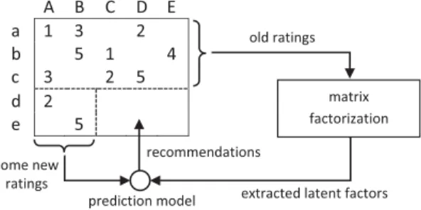
Figure 1: Recommender system using matrix fac-torizations.
For example, in the Lastfm dataset, the items are the artists in a music website. The latent factors could be the music genres. The recommender system first obtains the genres of the artists, and the users’ interests on different genres. Then the system makes recommendations by align-ing the user’s interests to the genres of the artists.
For ratings modeled as the matrixR, various matrix fac-torization techniques have been applied to extract the latent factors and make recommendations. Figure 1 shows a typ-ical recommender system using matrix factorization. The old ratings given by existing users are first decomposed into multiple matrices to extract the latent factors. When new users come into the system, their ratings are combined with the extracted latent factors to make recommendations.
Sarwar et al. [17] proposed one of the early works that use the low-rank Singular Value Decomposition (SVD) approx-imation to replace the missing values in the original rating matrix, i.e. R≈UlSlVlwhere the sizes of the matrices are
R: m×n,Ul:m×l,Sl: l×l, andVl:n×l. The diagonal ma-trixSlcontains thelbiggest singular values ofR, and this low-rank approximation is also called the truncated SVD. This approach relies on the fact that the rank-l truncated SVD approximation ˆR=UlSlVlminimizes the Frobenius normRˆ−RFamong all the rank-lmatrices, and we hope that the matrix ˆRwould generalize the correct ratings to the missing entries inR. Note that imputation of missing values is implicitly required when computing the truncated SVD. We can represent useriwith the vector ¯ui=Sl−1/2Ul(i,·) and itemk with the vector ¯vk =Sl−1/2Vl(i,·). The pre-dicted rating from userito itemkis then ˆR(i, k) = ¯uiv¯k, where ¯uiand ¯vkcan be considered as latent vectors.
During the Netflix prize competition, Funk [5] proposed an iterative way to compute the low-rank SVD
approxima-tion on a very big matrix that minimizes only the Frobenius norm on the non-empty entries in the original rating ma-trix. Based on Funk’s work, Paterek [14] suggested a new model to reduce the number of parameters that need to be stored in the recommender system. In Paterek’s approach, a truncated SVD is computed as before, but only the right singular vectors inVlare taken into the second step. In the second step, itemk is represented byvk which is the k-th column ofVl, while useri’s latent vector is computed by a linear combination of thevk’s whose corresponding items are rated by useri. Finally the rating prediction is the in-ner product of a user’s latent vector and an item’s latent vector. Koren [9] pointed out that this “asymmetric SVD” which takes only the right singular vectors actually works better in prediction accuracy. However, besides the empiri-cal studies, the reason of such improvement for asymmetric SVD is not clear.
Themain contributionsof this paper include(1)a new explanation of the (approximate) orthogonal structure of the latent space constructed from the asymmetric SVD, which is used as an intermediate step in a top-N recommender system, and(2) a novel algorithm based on a hypergraph formulation that brings more diversity in the recommenda-tions by applying normalizarecommenda-tions in the asymmetric SVD.
In the reminder of the paper, we start with the hyper-graph representation and the normalized hyperhyper-graph cut. We show that the asymmetric SVD approach follows the hypergraph learning scheme, and there is an (approximate) orthogonal structure associated with the right singular vec-tors. Based on the lengths of the latent vectors obtained from the right singular vectors, the items can be categorized into anchor items and non-anchor items. Finally we present a top-N recommendation algorithm that utilizes the above structures, and conduct experiments to compare our algo-rithm with the state-of-the-art approaches.
2.
PRELIMINARIES
Suppose we have two sets of entities: the user set Y =
{y1, y2, ..., ym}of sizem, and the item setZ ={z1, z2, ..., zn}
of sizen. The items in setZbelong tosclusters{C1, C2, ..., Cs}. Each cluster Cj is a subset ofZ andCj∩Cj =∅for j=j.
Taking the Lastfm dataset as an example again, let the setY be the set of users and the setZ be the set of artists. Clusters or partitions overZ can be established according to the genres of the artists. For example,C1 includes the rock music artists, while all the country music artists are in C2. Each user in the setY, on the other hand, is assumed to have a preference over music genres. If the user likes rock music, she would listen to the artists from C1 with high probability. If the user does not like country music, she would rarely listen to the artists fromC2.
The mutually exclusion between clusters of items is the basic assumption in our analysis. Each cluster can be con-sidered as a latent factor by which the ratings are generated. In some cases, however, an artist could play in multiple gen-res. This does not pose a problem to our basic assumption, because we can create a cluster (latent factor) that corre-sponds to a combination of genres. In fact, if the intuition behind the latent factors follows some categorical attributes, e.g. genres, languages, professions, etc., or a combination of categorical attributes, our basic assumption always holds.
A B C D E ୟ ୠ ୡ
A hypergraph from the old ratings. There are 3 hyperedges {ୟǡ ୠǡ ୡ}.
D B A
C
E
The induced graph from the hypergraph
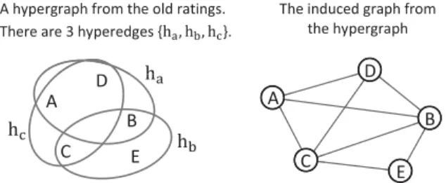
Figure 2: The hypergraph representation of the rat-ings in Figure 1 and the induced graph.
2.1
From Ratings to Relations
The matrixRcontains the ratings between the users and the items, which can be seen as relations between two sets. For simplicity, we assume that all the ratings are bigger than zero, thus the empty entries in them×nrating matrix R can be represented by zeros. If we ignore the actual ratings in R, we can obtain a binary matrix X = (R > 0) that represents only the relations, i.e. X(i, k) = 1 ifR(i, k)>0, otherwiseX(i, k) = 0, and the resulting matrix X can be precisely represented by a hypergraph.
Ahypergraph is an extension of a graph for modeling re-lations. In a graph, an edge connects exactly two vertices, while in a hypergraph ahyperedge connects any number of vertices. For a binary relation matrixX, the items are con-sidered as the vertices of a hypergraph, and a user is repre-sented by a hyperedge which contains all the items (vertices) that have been rated by the user. Following the tradition of visualizing a hypergraph in literatures, Figure 2 shows an example of the hypergraph representation. The matrixXis also called theincident matrix of the hypergraph. The ver-tex degree (of an item) is the sum of thek-th column ofX, i.e. deg(zk) =iX(i, k). Thehyperedge degree (of a user) is the sum of thei-th row ofX, i.e. deg(yi) =kX(i, k).
Recall that we assume there are some clusters of items, and these clusters correspond to the latent factors. Thus ex-tracting the latent factors is equivalent to finding clusters of items (vertices) in the hypergraph. There is a wide range of studies for clustering the vertices in a hypergraph [8, 1, 22]. In this paper, we focus on one particular line of studies that convert a hypergraph into an approximated graph so that the graph clustering algorithms can be applied to the hy-pergraph. Zhou et al. proposed a transformation to convert a hypergraph into a graph based on theNormalized Hyper-graph Cut (NHC) [22] (others include the clique-expansion, the start-expansion [1], and the hyperedge-expansion [15]). We denote the transformation proposed in [22] as “NHC”, and use it to find clusters in the hypergraph.
By applying the NHC transformation, the vertices of the hypergraph are copied into a new graph. Then each hyper-edge is converted into a clique of weighted hyper-edges in the new graph that connect all the vertices in the original hyperedge. The weights of the edges in the clique are normalized by the hyperedge degree so that the contribution of each hyperedge to the new graph is the same. With a linear combination of all the cliques from all the hyperedges, the new graph can be seen as an approximation of the hypergraph in the sense that any two vertices connected by some hyperedges are also connected in the new graph. We call this new graph theinduced graph (see Figure 2).
One can show that the adjacency matrix of the induced graph isXD−e1X, where X is the transpose ofX and De= diag (X1) is the hyperedge degree matrix. De is ac-tually the diagonal matrix of row sums of X, and1 is an all-ones vector of proper length. With the NHC transfor-mation, it is proposed to use the normalized Laplacian of the induced graph to find clusters of vertices [22], where the normalized Laplacian matrixLis defined as
L=I−D−v1/2XD−e1XD−v1/2. (1) MatrixIis an identity matrix, andDv= diag1Xis the vertex degree matrix.
As in standard spectral graph theory [4], the clustering algorithm involves computing the leading (smallest)l eigen-values{λ1, λ2, ..., λl}of Land the corresponding eigenvec-tors [f1,f2, ...,fl] =F. Then a vertex (or an itemzk) can be represented by a vector αk that is thek-th column of F(note thatF is of sizen×l). We call thel-dimensional vectorαkthelatent vector, and thel-dimensional space the
latent space. Once the latent vectors are computed, one can apply any clustering algorithm (such as k-means) in the la-tent space to find clusters of vertices.
This scheme of spectral technique (the list of eigenvalues are often called thespectrumof the matrix) has been widely used in many areas. It has close connections to the Principal Component Analysis (PCA), SVD, and many other matrix factorization techniques. In the next section, we show that the NHC transformation of a hypergraph is equivalent to a SVD, and under certain conditions there is a structure with the resulting latent vectors. Note that although the actual ratings are ignored in the hypergraph representation, they will be used again in the top-N recommendation algorithm presented in Section 4.
3.
HYPERGRAPH LEARNING USING SVD
The normalized LaplacianLis a symmetric matrix. Let ¯
X=D−e1/2XDv−1/2. (2) We can rewriteL=I−X¯X¯. The biggestleigenvalues of
¯
XX¯ are exactly{1−λ1,1−λ2, ...,1−λl}, while the cor-responding eigenvectors are still [f1,f2, ...,fl] = F. Then we decompose the matrix ¯X by the full SVD ¯X=USV, whereUandV are unitary matrices, andSis a rectangular diagonal matrix. The biggestl singular values inSare ex-actly {√1−λ1,
√
1−λ2, ..., √
1−λl}, and the columns of V (right-singular vectors) are the eigenvectors of ¯XX¯. Therefore, instead of computing the eigen-decomposition of L, we can obtainF from the SVD of ¯X, i.e. F is the sub-matrix of the firstlcolumns ofV.
Since we are looking for the right singular vectors of ¯X as-sociated with the largestlsingular values, computingF can be done by the truncated SVD ¯X ≈UlSlVl =UlSlF. Thus the NHC transformation is equivalent to the asymmet-ric truncated SVD of ¯X. We call the column vectors in ¯X the “profiles” of the items.
There are many advantages of using SVD to compute the αk’s (latent vectors) rather than the eigen-decomposition of L. Firstly, the matrix ¯Xis usually sparse, but ¯XX¯ might be non-sparse. Whennis large, the computational cost and storage cost of the eigen-decomposition might be impracti-cal. Secondly, there are existing approaches to implement SVD incrementally, which allows us to just compute the mi-nor changes when modifying ¯X.
3.1
A Special Case
We first consider a special case where all the items in one cluster are rated by the same set of users. In other words, each clusterCjis associated with a subset of users and these users have rated all the items inCj. We call this special case the “full concentrated case” because it can be modeled with a beta distribution with a small concentration parameter. If there aresclusters, the matrix ¯X can be written as
¯ X= [ ¯x 1· · ·x¯1 |C1|vectors ¯ x2· · ·x¯2 |C2|vectors · · · x ¯s· · ·x¯s |Cs|vectors ], (3)
where the column vectors in one cluster are all the same. We call the items in thesclusters theanchor itemsbecause they define the cluster centers and remain clustered in the latent space.
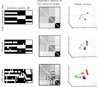
In spectral graph theory, if the graph containss discon-nected components, one can show that the latent vectors ob-tained from the first s eigenvectors of the graph Laplacian are aligned with the axes of thes-dimensional latent space [13]. When the disconnected components are connected by some weak links, the latent vectors are still aligned withs approximately orthogonal lines [20]. However, the induced graph of a hypergraph usually does not consist of more than one connected component. Figure 3 shows an example of a hypergraph in full concentrated case. The adjacency matrix of the induced graph is not a diagonal block matrix (not even approximately), so we need to develop a new analysis to support the clustering algorithm for hypergraphs.
incident matrixX
adjacency matrix of
the induced graph latent vectors
fu ll con c en trated case 5% n o ise 10% n o ise
Figure 3: Examples of the incident matrix and the latent vectors with the full concentrated case and noisy cases. The noises are added by randomly flip-ping some entries of X. Approximately orthogonal structures can be observed in the noisy cases. In the charts of latent vectors, the gray lines are from the origin to the cluster centers.
If the rank of ¯Xiss, i.e. the anchor item profiles ¯xj’s are linearly independent, the truncated SVD ¯X = UlSlVl is
an exact decomposition whenl=s. Recall that the latent vectors in F can be obtained fromF =Vl. The following statement shows the structure ofF.
Proposition 1. IfX¯ is in the form of Eq. (3) andx¯j’s are linearly independent, the latent vectorsF = [α1· · ·αn]
given by the truncated SVD X¯ =UsSsF (columns of F are normalized to 1) can be grouped by the clustersαk=βj
for∀zk∈Cj. The αk’s from the same cluster are identical (denoted asβj). Furthermore, we haveβjβj = 0for∀j= j, andβ
jβj =|Cj|−1 for∀j∈ {1,2, ..., s}. (See appendix for proof.)
If all the items are anchor items, i.e. in the form of Eq. (3) and having linearly independent ¯xj’s, the latent vectors would be in exactlys clusters whose centers are orthogonal to each other (see Figure 3). The length of the latent vector is the reciprocal of the cluster size. Unlike the graph case, the latent vectors computed from a hypergraph are usually not aligned with the axes of the latent space, but up to a rotation that depends on the cluster sizes and the distribu-tion of non-zero entries inX. Nevertheless, the orthogonal structure of the latent vectors still provides us a similar the-oretical foundation for clustering vertices as in the standard spectral graph theory.
3.2
More General Case
The assumption that all the items are anchor items is too strict. We usually have some item profiles which are combi-nations of some other item profiles. For example, there are pure “SciFi” books and pure “romance” books that attract distinct sets of readers (the anchor items). But one book might have the “SciFi” element and the “romance” element at the same time, so it could attract readers from both sets. The item profile of this book is apparently a combination of two profiles.
Besides the anchor items, we now consider thenon-anchor items that are combinations of anchor items. We assume that the weights of the combinations are always non-negative, which implies that only additions of profiles are allowed, but not subtractions. If there are n non-anchor items and s clusters of anchor items, ¯X can be rewritten as
¯ X= [ ¯x1· · · ·x¯n nvectors ¯ x1· · ·x¯1 |C1|vectors ¯ x2· · ·x¯2 |C2|vectors · · · x ¯s· · ·x¯s |Cs|vectors ], (4)
where the profile of non-anchor item zk is denoted as ¯xk (k ∈ {1,2, ..., n}), and the profile of an anchor item from cluster Cj is still denoted as ¯xj. Note that ¯xk is not an exact linear combination of the anchor items, because when combining the profiles of the anchor items, there might be redundant entries. For example, if ¯x1 = [1 1 0 0], ¯x2 = [0 1 1 0] and ¯xk is a combination of ¯x1 and ¯x2, ¯xk would be [1 1 1 0]instead of [1 2 1 0]because the incident matrix Xis always a binary matrix (normalizations are ignored in this example for simplicity). Thus we need to subtract the redundant entries when summing the anchor item profiles:
¯ x k= j∈I(z k) deg(zj) deg(zk)x¯j−r, (5) whereI(zk) is the set of anchor items from whichzk is con-structed, andr denotes the column vector that consists of the redundant entries in the profiles of the anchor items. Obviously all entries ofrare non-negative.
Denote the latent vector of an anchor item from clusterCj
asβj, and the latent vector of a non-anchor itemzk as βk.
By the SVD on ¯X,βk can be expressed by the combination β k= j∈I(z k) deg(zj) deg(zk)βj−S −1 l Ur. (6)
If the entries inrare small enough to be considered as resid-uals, or in other words the anchor items are associated with disjoint sets of users, we could still expect approximately or-thogonal structure between the latent vectors of the anchor items.
Proposition 2. If the anchor items are associated with
disjoint sets of users, i.e. x¯jx¯j = 0for∀j, j∈ {1,2, ..., s}, j =j, the latent vectors of the anchor items are approxi-mately orthogonalβjβj ≈0for∀j=j.
The conclusion of Proposition 2 follows from the fact that ¯
x
jx¯j = βjS2lβj = 0, and the first l singular values in Sl are approximately the same when the cluster sizes are
similar.
In practice, we can consider the anchor items as the most representative items of each cluster. For example, the pure “SciFi” books are the anchor items of the “SciFi” cluster, be-cause they have the most unique features that define what is “SciFi”. The anchor items are not necessarily the most popular items or the most informative items in each cluster, but the items that are most distant from all the other clus-ters and attract a very unique group of users. Usually the anchor items are in the long-tail part, i.e. less popular.
Although the anchor items exhibit the approximately or-thogonal structure, we do not know which items are the an-chor items. The following result suggests that it is possible to distinguish the anchor items and the non-anchor items by examining the length of the latent vectors.
Proposition 3. For a non-anchor itemzk, denoteI(zk)
the set of anchor items from whichzk is constructed. Sup-pose that the anchor items inI(zk)are non-overlapping, i.e.
¯ x
jx¯j = 0for∀j, j ∈I(zk), j=j, and the cluster sizes of the anchor items are similar, i.e. the lengths of the an-chor latent vectors are similar (denoted as βj2 ≈ b0 for ∀j∈I(zk), where·2 is thel2norm). We haveβk2< b0.
(See appendix for proof.)
This result states that the length of a non-anchor latent vector is smaller than the lengths of the anchor latent vectors from which the former is constructed. Therefore, we can find the anchor items by sorting the lengths of the latent vectors in descending order.
In order to verify the conclusions in Propositions 2 and 3, we compute the latent vectors by the rank-l truncated SVD of ¯X, and select 10·litems whose latent vectors have the longest lengths. Then the selected latent vectors are grouped into clusters by the k-means algorithm. By the conclusions of the Propositions, the cluster centers of the selected latent vectors should be approximately orthogonal. In Figure 4, we show the results from a real dataset with NHC and SVD. Because there is no hyperedge-degree and vertex-degree normalizations in SVD, the longest latent vec-tors are not necessarily the anchor items. We can observe that there exists an approximately orthogonal structure in the NHC results, while such structure is less clear with SVD. There are existing works about the categorization of the items or users based on their impact on the recommender
system, e.g. [12]. Our classification of anchor and non-anchor items provides a new perspective in the context of latent space. In summary,(1) if the latent vectors are all orthogonal, each corresponds to a different anchor item (the full concentrated case). (2) if they are not, there is an or-thogonal subset such that each latent vector in this sub-set corresponds to a different anchor item, and all the oth-ers (non-anchor items) are approximately in the subspace spanned by the orthogonal subset.(3)generally, the anchor items are rated by different groups of users.
Sc = 0.984 0 0.5 1 Sc = 0.814 0 0.5 1 NHC SVD
latent vectors (first 2d) clusters of anchor items
(a) (b)
Figure 4: The selected anchor items with longer la-tent vector lengths in the datasetBookCrossing (see Section 6 for the description of the dataset). (a) The anchor items are shown in red x-markers. (b) The cosine distance matrix of the clustered anchor items. Sc is the sum of average distances between clusters minus the sum of average distances within clusters, normalized by the largest possible value with a per-fect orthogonal structure. A Sc value close to 1 sug-gests a better orthogonal structure.
4.
THE NORMALIZED RELATIONAL SVD
We now present a new algorithm based on the NHC Lapla-cian and the above analysis. Once the latent vectors are computed for the items, we model the useryi’s interests (or latent profile) as another vectorθiin the same latent space. The predicted score for user yi on item zk is P(yi, zk) = θ
i αk, and the vector θi should take the values such that the predictor P coincides with the existing ratings (or as close as possible).
In order to simulate the scenario where the recommenda-tions are made for new users and evaluate the algorithm, we split the rating matrixRinto three parts
R= Rm Rtr,Rte }subsetYm }subsetYt . (7)
Firstly the users are separated into two subsets. Ym is the subset of old users, andYt is the subset of new users. The sub-matrixRmcontains all the ratings from the users inYm, and the ratings inRmare used for constructing the hyper-graph and computing the latent vectors. The ratings from the users inYtare further split into two parts: RtrandRte. Rtr contains the “known” ratings of the new users. Based
onRtrand the latent vectors, we can predict or recommend more items for the users in Yt. Then the predictions are evaluated by the ratings in Rte. Note that only Rm and Rtr are taken as the inputs of the algorithm. Rte is used for evaluation.
Since our algorithm works with the hypergraph transfor-mation and SVD, we call itHSVD, which contains the follow-ing steps:
Step 1: Compute thel-dimensional NHC transformation F by the truncated SVD ¯Xm ≈ UlSlF, where ¯Xm is computed from the binary matrixXm= (Rm>0) (see Eq. (2)). Normalize each of thelcolumns ofF to 1 (l2 norm).
Step 2: For each useryi∈Yt, we choose theθithat min-imizes the error Rtr(i,·)−θiF22. The predicted score vector is ˆri = θiF. In matrix form, the full prediction matrix is ˆRte=ΘF, whereΘis obtained by solving the linear systemFΘ=Rtrin a least-squares sense.
Step 3: For each user yi ∈ Yt, recommend the top-N unrated items with the highest scores in ˆRte.
There are several normalizations in the HSVD algorithm which did not exist in previous matrix factorization meth-ods. When computing ¯Xmin step 1, the hyperedge-degree normalization (from the induced graph transformation it-self) and the vertex-degree normalization (from the normal-ized Laplacian of the induced graph) ensure that the anchor latent vectors would have longer lengths. By Proposition 1, the normalization of the columns of F in step 1 is also indispensable for producing an (approximately) orthogonal structure in the latent space.
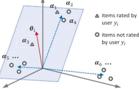
When computing theθi in step 2, two parts are actually taken into consideration, which is illustrated in Figure 5. Firstly we consider the latent vectors of the items which are rated by useryi(the triangle points in Figure 5). We would like to choose a θi that is close to these ratedαk’s. Since the row vectorR(i,·) is weighted by the ratings,θi should be even closer to theαk’s with higher ratings, which can be expressed as θi = arg minθk,R(i,k)>0
R(i, k)−θiαk2. Because every non-anchor item is approximately a linear combination of some anchor items (e.g. α3 is a combina-tion of α1 and α5 in Figure 5), θi should be in the sub-space spanned by the latent vectors of the underlying an-chor items. Secondly, for those αk’s that are not rated by user yi (the circle points in Figure 5), θi should stay as far from them as possible, ideally orthogonal to these un-rated latent vectors. The orthogonality between the clus-ter cenclus-ters of the anchor items suggests that it is possible to find a θi which is orthogonal to the anchor items that the user yi is not interested in. This can be expressed as θi = arg minθk,R(i,k)=0
θ
i αk2. Putting the two parts together, it suggests that in matrix form the θi’s can be obtained by solving the linear systemFΘ=Rtrin a least-squares sense, which is in the step 2 of theHSVDalgorithm.
ࣂ ࢻଵ ࢻଶ ࢻଷ ࢻସ ࢻହ ࢻ ହ… … items rated by user ݕ items not rated by user ݕ
Figure 5: Illustration of the HSVD algorithm in 3d latent space. The dashed lines are cluster centers of the anchor items.
Proposition 3 shows that the lengths of the anchor latent vectors are longer than the non-anchor latent vectors, even if the anchor items are less popular. For a fixedθi, because the score ˆRte(i, k) is simply the inner product ofθiandαk, the anchor items of longer length would have bigger chance to be selected in the top-Nrecommendations. This would allow us to diversify the recommendation list and recommend more less-popular items.
4.1
Scalability
The main computational cost of our algorithm comes from the truncated SVD routine. Usually the numerical method for truncated SVD on matrix ¯X is in an iterative manner, and operated as an eigen-decomposition of the Hermitian matrix ¯XX. The running time of the latter problem de-¯ pends on the complexity of each iteration and the total num-ber of iterations. In each iteration the basic operation con-tains two matrix vector multiplications ¯XXv¯ wherevis a dense vector. If the number of non-zero entries in ¯X (or the number of ratings inR) isM, the complexity of each itera-tion would beO(M). On the other hand, the total number of iterations to converge depends on the gap between thel largest singular value and thel+ 1 largest singular value. A bigger gap leads to a smaller number of iterations [6, 11]. If the number of iterations isnI, the overall complexity of the HSVDalgorithm isO(nIM), which is linear to the number of ratings. The parameterl (dimensionality of the truncated SVD) is considered as a constant, which can be determined by cross-validation in practice.
5.
RELATED WORK
In the introduction, we have mentioned the SVD [17], the SVD on non-empty entries [5], and the asymmetric SVD [14, 9] for recommender systems. Another matrix factorization technique that is widely used in recommender systems is thenon-negative matrix factorization(NMF). In NMF, the rating matrix is approximately decomposed into two low-rank, sparse and non-negative matrices R ≈ GH such that R−GH2 is minimized [7, 16]. The idea behind NMF is that the set of orthogonal latent factors controls the values in R, and each latent factor takes one axis in the latent space. This idea is essentially similar to theHSVD since we have shown that the anchor items also exhibit an orthogonal structure in the latent space, although they are not aligned to the axes.
In order to compare our algorithm with the existing ap-proaches, we adapt the SVD and the NMF into our setting, i.e. split the rating matrix into three parts as in Eq. (7) and use the sub-matrixR=RmRtrto compute the SVD or NMF, then evaluate the results onRte. The SVD and NMF algorithms in this setting are denoted asSVDRandNMFR.
To make a better baseline, we also apply the SVDR and NMFRonRmand predict withRtrin an asymmetric manner, i.e. follow the same procedures in Section 4 but replace ¯Xm withRm(or replaceF with the matrixHin NMF). These methods are denoted asASVDRandANMFR, where the leading “A” means “asymmetric”.
We use the routine implemented by TimelyDevelopment for computing the SVD on non-empty entries [18], which is denoted asSVDN. Note thatSVDNis exactly the same asSVDR except for the SVD computation routine.
For the asymmetric SVD, we use the approach proposed in [14]. In this approach, a decomposition is first computed
by SVDN R ≈UlSlVl, where Vl = [α1· · ·αn]. Then a
user yi is represented by the currently rated items: θi =
k,R(i,k)>0αk. Finally a score is computed by the rule ˆ
R(i, k) =ak+θi αk for each unrated item, whereakis the average rating of itemzk. We call this methodASVDN.
6.
EXPERIMENTAL RESULTS
In a top-N recommender system, the primary goal is to discover the unrated items that might be liked by a user [3]. We first test the algorithm’s ability to discover the unrated items, which is denoted as the scenario PREDICT-ALL. The rating matrix is split into three parts as in Eq. (7), and we randomly selectRtrto have 5 ratings in each row (for each user). The remaining ratings in theYt part are assigned to Rte. This setting simulates the situation where new users
just come into the system with only a few ratings, which is denoted as PREDICT-ON-5. Similarly, we create another settingPREDICT-ON-20where each row ofRtrhas 20 ratings to simulate the users with more available ratings. Thus in the scenario PREDICT-ALL, there are two settings, namely PREDICT-ON-5 andPREDICT-ON-20. Note that all the items inRte(rated or unrated) could be recommended in the top-Nrecommendation list. In all the experiments,RtrandRte
are randomly selected in 5 different runs.
To test the results, we check if the set of recommended items coincides with the liked items (ratings higher than the median) for each user in the corresponding row ofRte. Let
ˆ RN
i and Ri denote these two sets for user yi. We measure
the average precision precision = (1/|Yt|) yi∈Yt |RˆN i ∩Ri|/|RˆNi | . (8)
Lastfm YahooMusic BookCrossing
SVDR 0.113 0.083 0.237 0.207 0.078 0.063 ASVDR 0.114 0.087 0.237 0.210 0.078 0.062 NMFR 0.114 0.090 0.218 0.189 0.073 0.054 ANMFR 0.110 0.089 0.211 0.190 0.071 0.056 SVDN 0.002 0.003 0.001 0.001 0.005 0.003 ASVDN 0.003 0.002 0.007 0.005 0.005 0.003 HSVD 0.180 0.158 0.258 0.227 0.075 0.065
Table 1: Average precisions in PREDICT-ALL. The left column of each dataset: PREDICT-ON-5, the right col-umn: PREDICT-ON-20. The bold number indicates the method that performs significantly better than the others (p-value<0.05 in paired t-test).
Lastfm YahooMusic BookCrossing
SVDR 0.198 0.140 0.490 0.418 0.743 0.744 ASVDR 0.198 0.139 0.496 0.435 0.743 0.745 NMFR 0.541 0.545 0.763 0.774 0.731 0.740 ANMFR 0.279 0.222 0.579 0.496 0.743 0.745 SVDN 0.177 0.244 0.249 0.224 0.389 0.165 ASVDN 0.537 0.531 0.755 0.783 0.696 0.714 HSVD 0.515 0.524 0.765 0.766 0.745 0.747
Table 2: Average precisions in RANK-CANDIDATES. (see the caption of Table 1 for more details)
In the scenarioPREDICT-ALL, any item which is not inRtr can be considered in the recommendation list. But some-times we already know a set of candidate items that a user
has suggested implicitly. For example, a user has viewed a list of pages of artists, but did not make any further ac-tions like purchase a CD or download a track. In this case, we can limit our recommendations on the candidate items and only pick up the items that are truly liked by the user, which could be simulated by only recommending the rated items in Rte. We try to rank these items such that the liked ones are ranked higher. This scenario is denoted as RANK-CANDIDATES. The same measure (precision defined in Eq. (8)) is evaluated inRANK-CANDIDATES.
We have tested all the methods listed in Section 5 with the above settings on three datasets. Lastfm1 contains the relations between users and artists collected fromlast.fm, and the ratings inLastfmare the actual counts of plays with which a user has listened to an artist.YahooMusic2is also in the music domain, but includes relations between users and tracks. The ratings inYahooMusicare in the range of 1 to 100. The last datasetBookCrossing contains ratings from users to books [23]. The range of ratings inBookCrossing is from 1 to 10. In each dataset, we take a subset such that the induced graph of the hypergraph representation is connected. When the dataset contains a hypergraph with multiple connected components, we could simply apply the algorithm to each connected component respectively.
mean = 163.125
median = 144 mean = 190.845median = 178
mean = 164.202
median = 144 mean = 201.801median = 196
10 100 mean = 104.868 median = 73 10 100 mean = 131.698 median = 97 ˆ RN i RˆNi ∩Ri SVDR NMFR HSVD mean = 1123.961 median = 856 mean = 1509.753 median = 1237 mean = 1107.970
median = 824 mean = 1569.781median = 1272
10 100 1000 mean = 1023.088 median = 721 10 100 1000 mean = 1390.724 median = 1123 SVDR NMFR HSVD
more popular→ more popular→
Figure 6: The distribution of popularity of the items (in thePREDICT-ALLscenario withN= 20). The x-axis (popularity) is in log-scale. The mean and median of the popularity of the items are also shown in each sub-figure. Top: BookCrossing. Bottom: YahooMusic.
Table 1 and Table 2 show the results ofPREDICT-ALLand RANK-CANDIDATES respectively (withN = 20). In the first case, our proposed method performs best within the mu-sic domain, and shows results as good as the best methods with BookCrossing. The approaches ignoring the empty values (SVDNandASVDN) does not perform very well. These methods are originally designed to minimize the root mean squared error on a testing set of known ratings, which is not fully compatible with the scenarioPREDICT-ALL. In the 1
Available athttp://mtg.upf.edu/node/1671
2Yahoo! Webscope dataset ydata-ymusic-kddcup-2011-track2http://labs.yahoo.com/Academic_Relations
RANK-CANDIDATES, no method performs significantly better than the others over all datasets. But the NMF-based method NMFR and two asymmetric methodsASVDNand HSVDare al-ways as good as the best one.
In recommender systems, we are mainly interested in rec-ommending non-popular (long-tail) items, because the users are usually already aware of the popular items from other sources [19]. For the purpose of diversifying recommenda-tions, we measure the popularity distribution of the items in ˆRNi and ˆRiN∩Ri, i.e. the set of all recommended items and the set of successfully recommended items (Figure 6). The popularity of an item zk is the number of ratings in the k-th column of the rating matrix, i.e. deg(zk). We observe thatHSVD produces more diverse recommendations with the same (or better) level of precision. Especially with BookCrossing, there are much more less-popular recommen-dations fromHSVDcompared toSVDRandNMFR.
Figure 7 explains why our approach produces more di-verse recommendations. By using SVD without normaliza-tion, the lengths of the anchor items are not necessarily the longest ones. In fact, we can observe that there is a strong correlation between the popularity and the length of the latent vector with ASVDR, which would promote the popu-lar items in the recommendations. In our approach HSVD, the longest latent vectors correspond to the anchor items of smaller popularity. 0 100 200 300 400 500 0 0.05 0.1 0.15 0.2 0 100 200 300 400 500 0 0.1 0.2 0.3 0.4 HSVD ASVDR le ng th o f the la ten t v ecto r
popularity of the item popularity of the item
Figure 7: The length of the latent vectors and the popularity of all the items inBookCrossing.
7.
CONCLUSION
In this work, we present a new perspective of SVD for constructing a latent space from the training data, which is justified by the transformation of normalized hypergraph cut. We show that the latent vectors representing the items in the latent space can be grouped into (approximately) or-thogonal clusters, and the lengths of the vectors can be used to distinguish the anchor items and the non-anchor items. These properties are then utilized for making top-N recom-mendations in the proposed algorithmHSVD. Instead of ex-plicitly constructing the clusters, the recommendations are generated by solving a linear system. We provide new expla-nations for the significantly better performance of the asym-metric SVD approaches and better diversity in top-N rec-ommendations. Experiments conducted with three dataset on two domains also confirm our analysis.
Future works could include further studies of the latent space structures, and engineering methods that exploit such structures. For example, we can explicitly extract the anchor items to construct some clusters, and analyze the features of a non-anchor item by studying the underlying anchor clus-ters. It is also possible to include additional information,
e.g. contextual information [2] and social information [21], or rating bias corrections [10] into our scheme for further improvements.
8.
REFERENCES
[1] S. Agarwal, K. Branson, and S. Belongie. Higher order learning with graphs. InICML, 2006.
[2] L. Baltrunas, B. Ludwig, and F. Ricci. Matrix factorization techniques for context aware recommendation. InRecsys, 2011.
[3] P. G. Campos, F. D´ıez, and M. S´anchez-Monta˜n´es. Towards a more realistic evaluation: testing the ability to predict future tastes of matrix factorization-based recommenders. InRecsys, 2011.
[4] F. Chung.Spectral Graph Theory. American Mathematical Society, 1997.
[5] S. Funk. Netflix update: Try this at home,http:// sifter.org/∼simon/journal/20061211.html. 2006. [6] G. H. Golub and C. F. Van Loan.Matrix
computations. Johns Hopkins University Press, 1996. [7] P. Hoyer. Non-negative matrix factorization with
sparseness constraints.Journal of Machine Learning Research, 5:1457–1469, 2004.
[8] G. Karypis, R. Aggarwal, V. Kumar, and S. Shekhar. Multilevel hypergraph partitioning: Application in vlsi domain. InProc. of the 34th annual Design
Automation Conference, 1997.
[9] Y. Koren. Factorization meets the neighborhood: a multifaceted collaborative filtering model. In
SIGKDD, 2008.
[10] Y. Koren, R. Bell, and C. Volinsky. Matrix factorization techniques for recommender systems.
Computer, 42(8):30–37, 2009.
[11] D. Mavroeidis. Mind the eigen-gap, or how to accelerate semi-supervised spectral learning algorithms. InIJCAI, 2011.
[12] B. K. Mohan, B. J. Keller, and N. Ramakrishnan. Scouts, promoters, and connectors: The roles of ratings in nearest-neighbor collaborative filtering.
ACM Transactions on the Web, 1(2):8, 2007. [13] A. Y. Ng, M. I. Jordan, Y. Weiss, et al. On spectral
clustering: Analysis and an algorithm. InNIPS, 2002. [14] A. Paterek. Improving regularized singular value
decomposition for collaborative filtering. InProc. of KDD Cup and Workshop, 2007.
[15] L. Pu and B. Faltings. Hypergraph learning with hyperedge expansion. InECML-PKDD, 2012. [16] S. Rendle and L. Schmidt-Thieme. Online-updating
regularized kernel matrix factorization models for large-scale recommender systems. InRecsys, 2008. [17] B. Sarwar, G. Karypis, J. Konstan, and J. Riedl.
Application of dimensionality reduction in
recommender system-a case study. InWebKDD, 2000. [18] TimelyDevelopment.http://www.timelydevelopment
.com/demos/NetflixPrize.aspx. 2006.
[19] S. Vargas and P. Castells. Rank and relevance in novelty and diversity metrics for recommender systems. InRecsys, 2011.
[20] L. Wu, X. Ying, X. Wu, and Z. Zhou. Line
orthogonality in adjacency eigenspace with application to community partition. InIJCAI, 2011.
[21] Q. Yuan, L. Chen, and S. Zhao. Factorization vs. regularization: fusing heterogeneous social relationships in top-n recommendation. InRecsys, 2011.
[22] D. Zhou, J. Huang, and B. Scholkopf. Learning with hypergraphs: Clustering, classification, and
embedding. InNIPS, 2007.
[23] C. Ziegler, S. McNee, J. Konstan, and G. Lausen. Improving recommendation lists through topic diversification. InWWW, 2005.
APPENDIX
Proof for Proposition 1:
Firstly, it can be shown thatαk = αk if zk, zk ∈ Cj, because the k-th column and the k-th column of SsF must be the same to obtain the same ¯xk and ¯xk, which implies thatαk=αk. Secondly, we consider the full SVD of ¯X and list the rows ofV corresponding to items inCj:
V (j)= βj βj · · · βj γ1 γ2 · · · γ|Cj| . (9)
It is always possible to find a linear combination of the first s columns ofV (denoted as [f1,f2, ...,fs] =F) such that F tj=0· · ·1· · ·0, wheretjare the coefficients, and
the 1’s on the right hand side correspond to the items in Cj. Because all the columns in V are orthogonal to each other, a column is also orthogonal to a linear combination of some other columns (e.g. F tj). Thus the entries in each dimension of the vectors{γ1, ..., γ|Cj|}sum up to 0. In other words,k={1,2,...,|C j|}γk = 0, andV (j)1=|Cj| β j 0 . Since all the rows inV are also orthogonal to each other, we haveV(j)1V(j)1
= 0, which implies thatβjβj = 0. Proof for Proposition 3:
By Eq. (6) we know thatβk=j∈I(z
k)
deg(zj) deg(zk)βj(the residual r is zero because the involved anchor items are non-overlapping). Thus βk22 = j∈I(z k) deg(zj) deg(z k)βj 2 2+ j,j∈I(z k),j=j2 √ deg(zj)deg(zj) deg(z k) β
jβj. Since the anchor items are non-overlapping, we havej∈I(z
k)deg(zj) = deg(z
k).
The above equation can be written as
β k22=b 2 0+ j,j∈I(z k),j=j 2 deg(zj)deg(zj) deg(zk) β jβj. (10)
Following the proof for Proposition 1, it can be shown that β jβj= −1 |Cj||Cj| ⎛ ⎝ p∈I−1(j) deg(zj) deg(zp)β p ⎞ ⎠ ⎛ ⎝ q∈I−1(j) deg(zj) deg(zq)β q ⎞ ⎠, (11) where I−1(j) is the set of non-anchor items that contain a fraction of an anchor item in clusterCj. Since eachβpis a linear combination of theβj’s of the anchor items, and we know from Proposition 2 that βjβj ≈0 for∀j =j, it is easy to show that βjβj <0. Applying this result to Eq. (10), it concludes toβk2< b0.